JETSPIN: a specific-purpose open-source software for simulations of nanofiber electrospinning

Abstract

We present the open-source computer program JETSPIN, specifically designed to simulate the electrospinning process of nanofibers. Its capabilities are shown with proper reference to the underlying model, as well as a description of the relevant input variables and associated test-case simulations. The various interactions included in the electrospinning model implemented in JETSPIN are discussed in detail. The code is designed to exploit different computational architectures, from single to parallel processor workstations. This paper provides an overview of JETSPIN, focusing primarily on its structure, parallel implementations, functionality, performance, and availability.

1 Introduction

In the recent years, electrospun nanofibers have gained a considerable interest due to many potential industrial applications, such as tissue engineering, air and water filtration, drug delivery and regenerative medicine. In particular, the high surface area to material mass ratio of the fibers offers intriguing prospects for technological applications. As consequence, several studies have focused on the characterization and production of uni-dimensionally elongated nanostructures. A number of reviews [1, 2, 3, 4, 5] and books [6, 7, 8] concerning electrospinning have been published in the last decade.

Typically, electrospun nanofibers are produced at laboratory scale via the uniaxial stretching of a jet, which is ejected at a nozzle from an electrified polymer solution. Indeed, the initial elongation of the jet can be obtained by applying an external electrostatic field between the spinneret and a conductive collector. Electrospinning involves mainly two sequential stages in the uniaxial elongation of the extruded polymer jet: an initial quasi-steady stage, in which the electric field stretches the jet in a straight path away from the nozzle, and a second stage characterized by a bending instability induced by small perturbations, which misalign the jet away from its axis of elongation [9]. These small disturbances may originate from mechanical vibrations at the nozzle or from hydrodynamic-aerodynamic perturbations within the experimental apparatus. Such a misalignment provides an electrostatic-driven bending instability before the jet reaches the conductive collector, where the fibers are finally collected. As a consequence, the jet path length between the nozzle and the collector increases and the stream cross-section undergoes a further decrease. The ultimate goal of the electrospinning process are to control the cross-sectional radius and to maximize the uniformity of the collected fibers. By a simple argument of mass conservation, this is tantamount to maximizing the jet length by the time it reaches the collecting plane. By the same argument, it is therefore of interest to minimize the length of the initial stable jet region. Consequently, the bending instability is a desirable effect, as it produces a higher surface-area-to-volume ratio of the jet, which is transferred to the resulting nanofibers [10].

Recently, due to the broad interest of nanotechnology and to the wide application fields gained by polymer nanofibers even at industrial scale [5], electrospinning has attracted the attention of a large community of researchers, including modeling and computational aspects [11, 12, 13, 14, 15, 9]. In fact, computational models provide a useful tool to elucidate the physics of electrospinning and provide information which may be used for the design of new electrospinning experiments. Numerical simulations can also help improving the capability of predicting the role of the key process parameters and exert a better control on the resulting nanofiber structure. Although some authors used dissipative particle dynamics mesoscale simulation methods [16], various models treat the jet filament as a series of discrete elements (beads) obeying the equations of continuum mechanics [11, 12]. Each bead is subject to different types of interactions, such as long-range Coulomb repulsion, viscoelastic drag, the force related to the external electric field, and so on. The main aim of such models is to capture the complexity of the resulting dynamics and to provide the set of parameters driving the process. The effect of fast-oscillating loads on the bending instability has been also explored in an extensive computational study [17].

In recent works, we extended the unidimensional bead-spring model, developed by Pontrelli et al. [18], to include a nonlinear dissipative-perturbing force which models the effects of the air drag force. This has been accomplished by adding a random and a dissipative force to the equations of motion. In particular, we investigated both linear and non-linear Langevin-like models to describe air drag effects [19, 20].

Encompassing the previous efforts, in this paper we present, along with the overall model, a detailed algorithm and the corresponding FORTRAN code, JETSPIN, specifically designed to simulate the electrospinning process under a variety of different conditions and experimental settings. This comprehensive platform is devised in such a way to handle a variety of different cases via a suitable choice of the input variables. The framework is developed to exploit several computational architectures, both serial and parallel. With most of parameters taken from relevant literature in the field, a number of test cases have been carried out and an excellent agreement with experiments has been found.

JETSPIN, as open-source software, can be used to carry out a systematic sensitivity analysis over a broad range of parameter values. The results of simulations provide valuable insight on the physics of the process and can be used to assess experimental procedures for an optimal design of the equipment and to control processing strategies for technologically advanced nanofibers.

2 Structure

JETSPIN is written in free format FORTRAN90, and it consists of approximately 140 subroutines. The source exploits the modular approach provided by the programming language. All the variables having in common description of certain features or method are grouped in modules. The convention of explicit type declaration is adopted, and all the arguments passed in calling sequences of functions or subroutines have defined intent. We use the PRIVATE and PUBLIC accessibility attributes in order to decrease error-proneness in programming.

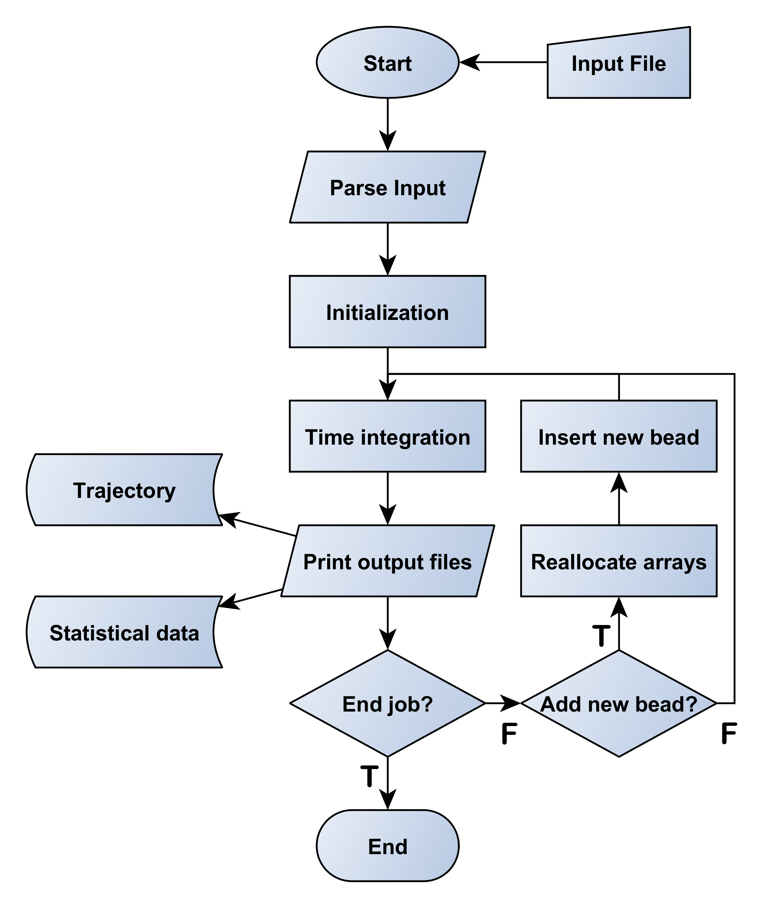
Figure 1: Structure of the main JETSPIN program.

The main routines have been gathered in the main.f90 file, which drives all the CPU-intensive computations needed for the capabilities mentioned below. The variables describing the main features of jets (position, velocity, etc.) are declared in the nanojet_mod.f90 file, which also contains the main subroutines for the memory management of the fundamental data of the simulated system. Since the size system is strictly time-dependent, JETSPIN exploits the dynamic array allocation features of FORTRAN90 to assign the necessary array dimensions. In particular, the size system is modified by the routines add_jetbead and erase_jetbead, while the decision of the main array size, declared as mxnpjet, is handled by the routine reallocate_jet. The sizes of various service bookkeeping arrays are handled within a parallel implementation strategy, which exploits few dedicated subroutines (see Sec 3). All the implemented time integrators are written in the integrator_mod.f90 file, which contains the routine driver_integrator to select the proper integrator, as indicated in the input file. All the terms of equations of motion for the implemented model (see Sec 4) are computed by routines located in the eom_mod.f90 file, which call other subroutines in the files coulomb_force_mod.f90, viscoelastic_force_mod.f90 and support_functions_mod.f90. A summarizing scheme of the main JETSPIN program in the main.f90 file has been sketched in Fig1.

The user can carry out simulations of electrospun jets without a detailed understanding of the structure of JETSPIN code. All the parameters governing the system can be defined in the input file (see Sec 5), which is read by routines located in the io_mod.f90 and parse_mod.f90 files. Instead, the user should be acquainted with the model described in Sec 4. The content of the output file is completely customizable by the input file as described in Sec 5, and it can report different time-averaged observables computed by routines of the module statistic_mod (see Sec 6). The routines in the error_mod.f90 file can display various warning or error banners on computer terminal, so that the user can easily correct the most common mistakes in the input file.

JETSPIN is supplied as a single UNIX compressed (tarred and gzipped) directory with four sub-directories. All the source code files are contained in the source sub-directory. The examples sub-directory contains different test cases that can help the user to edit new input files. The build sub-directory stores a UNIX makefile that assembles the executable versions of the code both in serial and parallel version with different compilers. Note that JETSPIN may be compiled on any UNIX platform. The makefile should be copied (and eventually modified) into the source sub-directory, where the code is compiled and linked. A list of targets for several common workstations and parallel computers can be used by the command "make target ", where target is one of the options reported in Tab 1. On Windows system we advice the user to compile JETSPIN under the command-line interface Cygwin [21]. Finally, the binary executable file can be run in the execute sub-directory.

3 Parallelization

The parallel infrastructure of JETSPIN incorporates the necessary data distribution and communication structures. The parallel strategy underlying JETSPIN is the Replicated Data (RD) scheme[22], where fundamental data of the simulated system are reproduced on all processing nodes. In simulations of electrospinning, the fundamental data consist of position, velocity, and viscoelastic stress arrays at each bead in which the jet is discretised (see below Sec 4). Further data defining mass and charge of each bead are also replicated. However, all auxiliary data are distributed in equal portion of data (as much as possible) for each processor. Despite other parallel strategies being available such as the Domain Decomposition[23], our experience has shown that such volume of data is by no means prohibitive on current parallel computers.

By the RD scheme, we implement the following parallel procedure: 1) A set of arrays (in the following text referred to as global arrays) containing position, velocity, viscoelastic stress, mass and charge of each bead is replicated on each processing node. 2) The routine set_chunk distributes the computational work over all the nodes by assigning a nanofiber chunk to each node. In particular, the first and last beads of the jet chunk dealt by the $i-th$ node are declared as mystart and myend, which have different values for each node. 3) Each node evolves in time the nanofiber for its assigned chunk of jet. Thus, the set of global arrays are updated only for the jet chunk which is handled by the specific node, while all the remaining values are set to zero. At this stage each node exploits service bookkeeping arrays which are not replicated, and whose size is dynamically allocated on the basis of the chunk size in order to save memory space. 4) Finally, global summation routines are employed in order to make the updated data of the global arrays available to all nodes. Note that we adopt in JETSPIN a simple strategy of communication between nodes, which is handled by global summation routines.

The module version_mod located in the parallel_version_mod.f90 file contains all the global communication routines which exploit the MPI (Message Passing Interface) library. It is worth stressing that a FORTRAN90 compiler and an MPI implementation for the specific machine architecture are required in order to compile JETSPIN in parallel mode. An alternative version of the module version_mod is located in the serial_version_mod.f90 file, and it can be easily selected by appropriate targets in the makefile at compile time (see Tab 1). By selecting this version, JETSPIN can also be run on serial computers without modification, even though the code has been designed to run on parallel computers.

The size system is strictly time-dependent as mentioned in Sec 2 and, therefore, the memory of various service bookkeeping arrays is dynamically distributed over all the processing nodes. In particular, the bookkeeping array size, declared as mxchunk, is managed by the routine set_mxchunk. All the beads of the discretised jet are assigned at every time step to a specific node by the routine set_chunk, and their temporary data are stored in bookkeeping arrays belonging to the assigned node. It is worth stressing that the communication latency makes the parallelization efficiency strictly dependent on the system size. Therefore, we only advice the use of JETSPIN in parallel mode whenever the user expects a system size with at least 50 beads for each node (further details in Sec 8).

4 Overview of model

4.1 Equations of motion

The model implemented in JETSPIN is an extension of the Lagrangian discrete model introduced by Reneker et al. [11]. The model provides a compromise of efficiency and accuracy by representing the filament as a series of $n$ beads (jet beads) at mutual distance $l$ connected by viscoelastic elements. The length $l$ is typically larger than the cross-sectional radius of the filament, but smaller than the characteristic lengths of other observables of interest (e.g. curvature radius). Each $i-th$ bead has mass $m_{i}$ and charge $q_{i}$ (not necessarily equal for all the beads). Evaporation has been neglected since it is not expected to introduce qualitative changes the jet dynamics [11]. However, the effect of solvent evaporation likely leads to a slight solidification of the jet, altering the rheological parameters of the polymer solution. This latter issue was addressed by an ad-hoc evaporation model proposed by Yarin et al. [24], whose implementation in JETSPIN will be considered in future releases. The jet is modelled as a viscoelastic Maxwell fluid, so that the stress $\sigma_{i}$ for the element connecting bead $i$ with bead $i+1$ is given by the viscoelastic constitutive equation:

$$\frac{d\sigma_{i}}{dt}=\frac{G}{l_{i}}\frac{dl_{i}}{dt}-\frac{G}{\mu}\sigma_{i},$$ (1)

where $l_{i}$ is the length between the bead $i$ with the bead $i+1$, $G$ is the elastic modulus, $\mu$ is the viscosity of the fluid jet, and $t$ is time. Given $a_{i}$ the cross-sectional radius of the filament at the bead $i$, the viscoleastic force $\vec{\textbf{f}}_{\upsilon e}$ pulling bead $i$ back to $i-1$ and towards $i+1$ is

$$\vec{\textbf{f}}_{\upsilon e,i}=-\pi a_{i}^{2}\sigma_{i}\cdot\vec{\textbf{t}}_{i}+\pi a_{i+1}^{2}\sigma_{i+1}\cdot\vec{\textbf{t}}_{i+1}\text{,}$$ (2)

where $\vec{\textbf{t}}_{i}$ is the unit vector pointing bead $i$ from bead $i-1$. The surface tension force $\vec{\textbf{f}}_{st}$ for the $i-th$ bead is given by

$$\vec{\textbf{f}}_{st,i}=k\cdot\pi\left(\frac{a_{i}+a_{i-1}}{2}\right)^{2}\alpha\cdot\vec{\textbf{c}}_{i}\text{,}$$ (3)

where $\alpha$ is the surface tension coefficient, $k$ is the local curvature, and $\vec{\textbf{c}}_{i}$ is the unit vector pointing the center of the local curvature from bead $i$. Note the force $\vec{\textbf{f}}_{st}$ is acting to restore the rectilinear shape of the bending part of the jet.

In the electrospinning experimental configuration an intense electric potential $V_{0}$ is applied between the spinneret and a conducting collector located at distance $h$ from the injection point. As consequence, each $i-th$ bead undergoes the electric force

$$\vec{\textbf{f}}_{el,i}=e_{i}\frac{V_{0}}{h}\cdot\vec{\textbf{x}}\text{,}$$ (4)

where $\vec{\textbf{x}}$ is the unit vector pointing the collector from the spinneret assuming a vertical $x$ axis starting at the spinneret ($x=0$). Note that in Ren model the intense electric potential $V_{0}$ is assumed to be static in order to avoid the computationally expensive integration of Poisson equation, whereas in reality $V_{0}$ is depending on the net charge of the jet so as to maintain constant the potential at the electrodes. The latter issue was elegantly addressed by Kowalewski et al. [25], and its implementation in JETSPIN will be planned. Furthermore, a model using a lattice method for electromagnetic wave propagation [26, 27, 28] is planned to be implemented in future releases in order to deal with electrospinning process in the presence of oscillating electric fields.

The net Coulomb force $\vec{\textbf{f}}_{c}$ acting on the $i-th$ bead from all the other beads is given by

$$\vec{\textbf{f}}_{c,i}=\sum_{\begin{subarray}{c}j=1\\ j\neq i\end{subarray}}^{n}\frac{q_{i}q_{j}}{R_{ij}^{2}}\cdot\vec{\textbf{u}}_{ij}\text{,}$$ (5)

where $R_{ij}=\left[\left(x_{i}-x_{j}\right)^{2}+\left(y_{i}-y_{j}\right)^{2}+\left(z_{i}-z_{j}\right)^{2}\right]^{1/2}$, and $\vec{\textbf{u}}_{ij}$ is the unit vector pointing the $i-th$ bead from $j-th$ bead.. Although the Reneker model provides a reasonable description for the spiral motion of the jet, the last term $\vec{\textbf{f}}_{c}$ introduces mathematical inconsistencies due to the discretization of the fiber into point-charges. Indeed, the charge induces a field on the outer shell of the fiber and not on the center line (as in the implemented model). Different approaches were developed to overcome this issue which usually imply strong approximations[29, 10, 30]. Other strategies use a less crude approximation by accounting for the actual electrostatic form factors between two interacting sections of a charged fiber[31] or involving more sophisticated methods which exploit the tree-code hierarchical force calculation algorithm[25]. The implementation of methods based on tree-code hierarchical force calculation algorithm in JETSPIN will be considered in future.

Although usually much smaller than the other driving forces, the body force due to the gravity is computed in the model by the usual expression

$$\vec{\textbf{f}}_{g,i}=m_{i}g\cdot\vec{\textbf{x}},$$ (6)

where $g$ is the gravitational acceleration.

The combined action of these forces governs the elongation of the jet according to the Newton’s equation:

$$m_{i}\frac{d\vec{\boldsymbol{\upsilon}}_{i}}{dt}=\vec{\textbf{f}}_{el,i}+\vec{\textbf{f}}_{c,i}+\vec{\textbf{f}}_{\upsilon e,i}+\vec{\textbf{f}}_{st,i}+\vec{\textbf{f}}_{g,i}\>\text{,}$$ (7)

where $\vec{\boldsymbol{\upsilon}}_{i}$ is the velocity of the $i-th$ bead. The velocity $\vec{\boldsymbol{\upsilon}}_{i}$ satisfies the kinematic relation:

$$\frac{d\vec{\textbf{r}}_{i}}{dt}=\vec{\boldsymbol{\upsilon}}_{i}$$ (8)

where $\vec{\textbf{r}}_{i}$ is the position vector of the $i-th$ bead, $\vec{\textbf{r}}_{i}=x_{i}\vec{\textbf{x}}+y_{i}\vec{\textbf{y}}+z_{i}\vec{\textbf{z}}$. The three Eqs 1, 7 and 8 form the set of equations of motion (EOM) governing the time evolution of system.

Depite the experimental evidence that the air drag affects the jet dynamics [32], the effects of aerodynamics are neglected at this stage. An extended stochastic model, recently developed in Refs [19, 20], including air drag effects is already planned for the next version of JETSPIN.

4.2 Perturbations at the nozzle

The spinneret nozzle is represented by a single mass-less point of charge $\bar{q}$ fixed at $x=0$ (nozzle bead). Its charge $\bar{q}$ is assumed equal to the mean charge value of the jet beads. Such charged point can be also interpreted as a small portion of jet which is fixed at the nozzle. In JETSPIN it is possible to add small perturbations to the $y_{n}$ and $z_{n}$ coordinates of the nozzle bead in order to model fast mechanical oscillations of the spinneret[17]. Given the initial position of the nozzle

$$y_{n}=A\cdot\cos\left(\varphi\right)$$ (9a)

$$z_{n}=A\cdot\sin\left(\varphi\right),$$ (9b)

the equations of motion for the nozzle bead are

$$\frac{dy_{n}}{dt}=-\omega\cdot z_{n}$$ (10a)

$$\frac{dz_{n}}{dt}=\omega\cdot y_{n},$$ (10b)

where $A$ denotes the amplitude of the perturbation, while $\omega$ and $\varphi$ are its frequency and initial phase, respectively.

4.3 Jet insertion

The jet insertion at the nozzle is modelled as follows. For sake of simplicity, let us consider a simulation which starts with only two bodies: a single mass-less point fixed at $x=0$ representing the spinneret nozzle, and a bead modelling an initial jet segment of mass $m_{i}$ and charge $e_{i}$ located at distance $l_{step}$ from the nozzle along the $x$ axis. Here, $l_{step}$ denotes the length step used to discretise the jet in a sequence of beads. The starting jet bead is assumed to have a cross-sectional radius $a_{0}$, defined as the radius of the filament at the nozzle before the stretching process. Applying the condition of conservation of the jet volume, the relation $\pi a_{i}^{2}\,l_{i}=\pi a_{0}^{2}l_{step}$ is valid for any $i-th$ bead. Furthermore, the starting jet bead has an initial velocity $\upsilon_{s}$ along the $x$ axis equal to the bulk fluid velocity in the syringe needle. Once this traveling jet bead is a distance of $2\cdot l_{step}$ away from the nozzle, a new jet bead (third body) is placed at distance $l_{step}$ from the nozzle along the straight line joining the two previous bodies. Let us now label $i-1$ the farthest bead from the nozzle, and $i$ the last inserted bead. The $i-th$ bead is inserted with the initial velocity $\upsilon_{i}=\upsilon_{s}+\upsilon_{d}$, where $\upsilon_{d}$ denotes the dragging velocity computed as

$$\upsilon_{d}=\frac{\upsilon_{i-1}-\upsilon_{s}}{2}.$$ (11)

Here, the dragging velocity should be interpreted as an extra term which accounts for the drag effect of the electrospun jet on the last inserted segment. Note that the actual dragging velocity definition was chosen in order to not alter the strain velocity term $\left(1/l_{i-1}\right)\cdot\left(dl_{i-1}/dt\right)$ of Eq 1 before and after the bead insertion.

4.4 Dimensionless quantities

In JETSPIN all the variables are automatically rescaled and stored in dimensionless units. In order to adopt a dimensionless form of the equations of motion, we use the dimensionless scaling procdure proposed by Reneker et al.[11]. We define a characteristic length

$$L_{0}=\sqrt{\frac{\bar{q}^{2}}{\pi a_{0}^{2}G}}=l_{step}\sqrt{\frac{\pi a_{0}^{2}\rho_{V}^{2}}{G}},$$ (12)

where we write the charge $q$ as $\pi a_{0}^{2}l_{step}\rho_{V}$, denoting $\rho_{V}$ the electric volume charge density of the filament. Further, we divide the time $t$ and the stress $\sigma$ by their respective characteristic scales reported in Tab2. By using the volume conservation condition, and introducing the dimensionless variables in EOM, we obtain:

$$\frac{d\vec{\bar{\textbf{r}}}_{i}}{d\bar{t}}=\vec{\boldsymbol{\bar{\upsilon}}}_{\,i}$$ (13a)

$$\frac{d\bar{\sigma}_{i}}{d\bar{t}}=\frac{1}{\bar{l}_{i}}\frac{d\bar{l}_{i}}{d\bar{t}}-\bar{\sigma}_{i}$$ (13b)

$$\frac{d\vec{\boldsymbol{\bar{\upsilon}}}_{\,i}}{d\bar{t}}= V\cdot\vec{\textbf{x}}+\sum_{\begin{subarray}{c}j=1\\ j\neq i\end{subarray}}^{n}\frac{Q_{ij}}{\bar{R}_{ij}^{2}}\cdot\vec{\textbf{u}}_{ij}-L_{step}F_{ve,i}\frac{\bar{\sigma}_{i}}{\bar{l}_{i}}\cdot\vec{\textbf{t}}_{i}+L_{step}F_{ve,i+1}\frac{\bar{\sigma}_{i+1}}{\bar{l}_{i+1}}\cdot\vec{\textbf{t}}_{i+1}+$$ (13c)

$$+L_{step}A_{i}\frac{\bar{k}}{4}\left(\frac{1}{\sqrt{\bar{l}_{i}}}+\frac{1}{\sqrt{\bar{l}_{i-1}}}\right)^{2}\cdot\vec{\textbf{c}}_{i}+F_{g}\cdot\vec{\textbf{x}}$$

where we used the dimensionless derived variables and groups defined in Tab2. It is worth stressing that the viscoelastic and surface tension force terms are slightly different from the dimensionless form provided by Reneker et al. [11], since we are considering the most general case $l_{step}\neq L.$

Similarly, the equations of motion of the nozzle become

$$\frac{d\bar{y}_{i}}{d\bar{t}}=-K_{s}\cdot\bar{z}_{i}$$ (14a)

$$\frac{d\bar{z}_{i}}{d\bar{t}}=K_{s}\cdot\bar{y}_{i}\>,$$ (14b)

with the dimensionless parameter $K_{s}$ defined in Tab2.

4.5 Integration schemes

In order to integrate the homogeneous differential EOM we discretise time as $t_{i}=t_{0}+i\Delta t$ with $i=1,\ldots,n_{steps}$, where $n_{steps}$ denotes the number of sub-intervals. In JETSPIN three different integration schemes can be exploited: the first-order accurate Euler scheme, the second-order accurate Heun scheme (sometimes called second-order accurate Runge-Kutta), and the fourth-order accurate Runge-Kutta scheme[33]. The user can select a specific scheme by using appropriate keys in the input file, as described in Sec 5. In addition, the time step $\Delta t$ is automatically rescaled by the quantity $\tau$, in accordance with the mentioned dimensionless scaling convention.

5 Description of input file

In order to run JETSPIN simulations an input file has to be prepared, which is free-form with no sequence field and case-insensitive. The input file has to be named input.dat, and it contains the selection of the model system, integration scheme directives, specification of various parameters for the model, and output directives. The input file does not requires a specific order of key directives, and it is read by the input parsing module. Every line is treated as a command sentence (record). Records beginning with the symbol # (commented) and blank lines are not processed, and may be added to aid readability. Each record is read in words (directives and additional keywords and numbers), which are recognized as such by separation by one or more space characters.

As in the example given in input test, the last record is a finish directive, which marks the end of the input data. Before the finish directive, a wide list of directives may be inserted (see Appendix A). The key systype should be used to set the jet model. In JETSPIN two models are available: 1) the one dimensional model similar to the model of Sec 4 but assuming the jet to be straight along the $\vec{\textbf{x}}$ axis, and, therefore, neglecting the surface tension force $\vec{\textbf{f}}_{st}$; 2) the three dimensional model described in Sec 4. Internally these options are handled by the integer variable systype, which assumes the values explained in Appendix A. Further details of the 1-D model can be found in Refs [18, 34]. A series of variables are mandatory and have to be defined. For example, timestep, final time, initial length, etc. (see underlined directives in Appendix A). A missed definition of any mandatory variable will call an error banner on the terminal. Given the mandatory directive initial length, the user can define the initial jet geometry in two ways: 1) the discretization step length is specified by the directive resolution, which causes automatically the setting of the jet segments number (the number of segment in which the jet is discretised); 2) the jet segments number is declared by the directive points, while the value of the discretization step length is automatically set by the program (as in Example input 3). The directive cutoff indicates the length of the upper and lower proximal jet sections, which interact via Coulomb force on any bead. It is worth stressing that the length value is set at the nozzle, so that the effective cutoff increases along the simulation as the jet is stretched.

The user should pay special attention in choosing the time integration step given by the directive timestep, whose detailed considerations are provided in Subsec 7.1. The reader is referred to Appendix A for a complete listing of all directives defining the electrospinning parameters. Not all these quantities are mandatory, but the user is informed that whenever a quantity is missed, it is usually assumed equal to zero by default (exceptions are stressed in Appendix A). Note that in the current software version all the quantities have to be expressed in centimeter–gram–second unit system (e.g. charge in statcoulomb, electric potential in statvolt, etc.).

6 Description of output files

A series of specific directives causes the writing of output files (see Appendix A). In JETSPIN two output files can be written: 1) the file statdat.dat containing time-dependent statistical data of simulated process; 2) the file traj.xyz reporting the jet trajectory in XYZ file format.

Various statistical data can be written on the file statdat.dat , and the user can select them in input using the directive printstat list followed by appropriate symbolic strings, whose list with corresponding meanings is reported in Appendix B. The statistical observables will be printed as mean values averaged over the time interval indicated by the directive print time, and reported on the same line following the order specified in input file. In the same way, a list of statistical data can be printed on computer terminal using the directive print list followed by the symbolic strings of Appendix B.

The file traj.xyz is written as a continuous series of XYZ format frames taken at time interval, so that it can be read by suitable visualization programs (e.g. VMD-Visual Molecular Dynamics [35], UCSF Chimera [36], etc.) to generate animations. The number of elements contained in the file is kept constant equal to the value specified by the directive print xyz maxnum, since few programs (e.g. VMD) do not manage a variable number of elements along simulations. If the actual number of beads is lower than the given constant maxnum, the extra elements are printed in the origin point.

7 Numerical tests

Here, we show three different examples of simulations. Each example addresses a specific issue of the jet model: 1) the choice of a suitable time step for the integration scheme; 2) the choice of a suitable length step for the jet discretization in order to properly approach the continuum jet description; 3) Fidelity of the model in reproducing experimental data.

7.1 Numerical accuracy and time step

Now, we intend to assess a typical time step value, $\Delta t$, for the integration schemes implemented in JETSPIN. To this purpose, exploiting the time reversibility and using dimensionless quantities, we integrate Eqs 13a, 13b and 13c forward for $n_{steps}$ time steps, and backward for further $n_{steps}$ time steps in the interval $\bar{t}_{a}=0$ and $\bar{t}_{b}=5$. Finally, we compute the average absolute error

$$\Delta\bar{x}=\left(\frac{1}{2n_{steps}}\right)\left|\bar{x}_{2n_{steps}}-\bar{x}_{0}\right|,$$ (15)

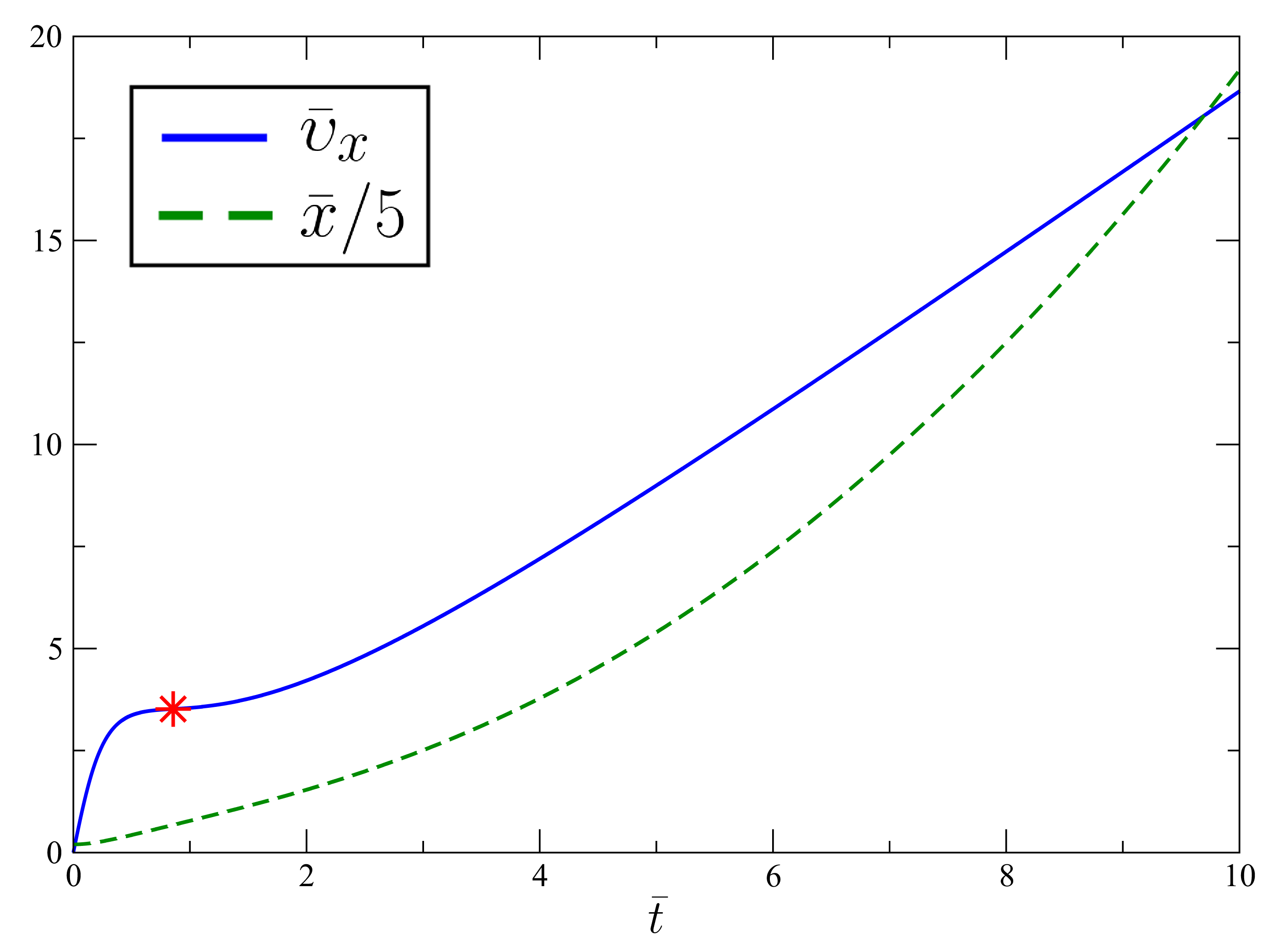
Figure 2: Time evolution of the velocity $\bar{\upsilon}_{x}$ (continuous line) and the length $\bar{x}$ rescaled by a factor $1/5$ (dotted line). Two stages of the elongation process are observed. The first stage comes to a quasi stationary point (denoted by a red star symbol). Then, in the second stage, the velocity comes to a near linearly increasing regime. The characteristic time and length scales are equal to $0.01\,\text{s}$ and $0.319\,\text{cm}$, respectively.

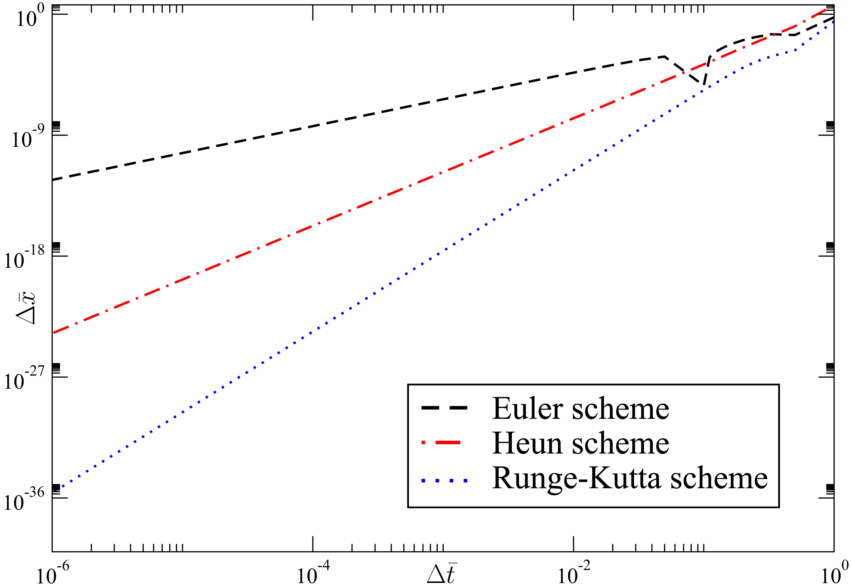
Figure 3: Deviation of the conserved quantity $\Delta\bar{x}$ versus time step $\Delta\bar{t}$ in log-log plot obtained by using the Euler scheme (black line), Heun scheme (red line), and Runge-Kutta scheme (blue line). The characteristic time and length scales are equal to $0.01\,\text{s}$ and $0.319\,\text{cm}$, respectively.

where $\bar{x}$ is the dimensionless position (defined in Subsec 4.4) along the $x$ axis of the bead (describing the jet) from the nozzle (located at zero). Here, $\bar{x}_{0}$ and $\bar{x}_{2n_{steps}}$ denote respectively the position of the jet bead at the beginning and at the end of the time integration. Note a perfect integrator ideally recovers $\bar{x}_{0}$ after $2n_{steps}$ time steps, so that we should obtain $\Delta\bar{x}=0$. The procedure was performed on the input example labeled input 1, and it was repeated for different values of time step $\Delta\bar{t}$. This input file provides the dimensionless parameter values $Q=12$, $V=2$ and $F_{ve}=12$, which have been already used as reference case in Refs [11, 18]. All the simulations start with the initial conditions $\bar{x}=1$, $\bar{\sigma}=0$, and $\bar{\upsilon}_{x}=0$. For sake of completeness, we report in Fig2 the time evolution of the position $\bar{x}$ and velocity $\bar{\upsilon}_{x}$. As already noted in Refs [11, 18], we identify two sequential stages in the elongation process. In the first regime, we observe a little increase of $\bar{\upsilon}_{x}$ which rises up to achieve a quasi stationary point, where the viscoelastic force balances the sum of the Coulomb and electric forces (due to the external electric field), providing a nearly zero value of the total force. Then, in the second stage the velocity trend comes to a near linearly increasing regime. In Fig3 we report the logarithmic trend of $\Delta\bar{x}$ versus $\Delta\bar{t}$ for the three different integration schemes. Here, the characteristic time and length scales are equal to $0.01\,\text{s}$ and $0.319\,\text{cm}$, respectively. As expected, we note a

precision of the Runge-Kutta scheme, while the computational cost increases by increasing the accuracy of the integration scheme, as discussed in more detail in Sec 8. The Euler’s method shows a lower numerical accuracy at larger values of $\Delta\bar{t}$, in particular close to $\Delta\bar{t}=10^{-1}$. The Heun scheme provides a compromise of efficiency and accuracy, keeping the absolute error $\Delta\bar{x}$ lower than $10^{-12}$ already for time step $\Delta\bar{t}=10^{-2}$. However, a good practice would be to perform preliminary tests of accuracy and efficiency for any specific case, since the accuracy is dependent on the magnitude of the dimensionless parameters.

7.2 Discretization length step

The discretization length step plays an important role, since we describe a continuous material system (the jet) by a series of discrete bodies. In particular, decreasing the discretization length step $l_{step}$, we approach the continuous description of the problem, and, therefore, an asymptotic behavior should be observed.

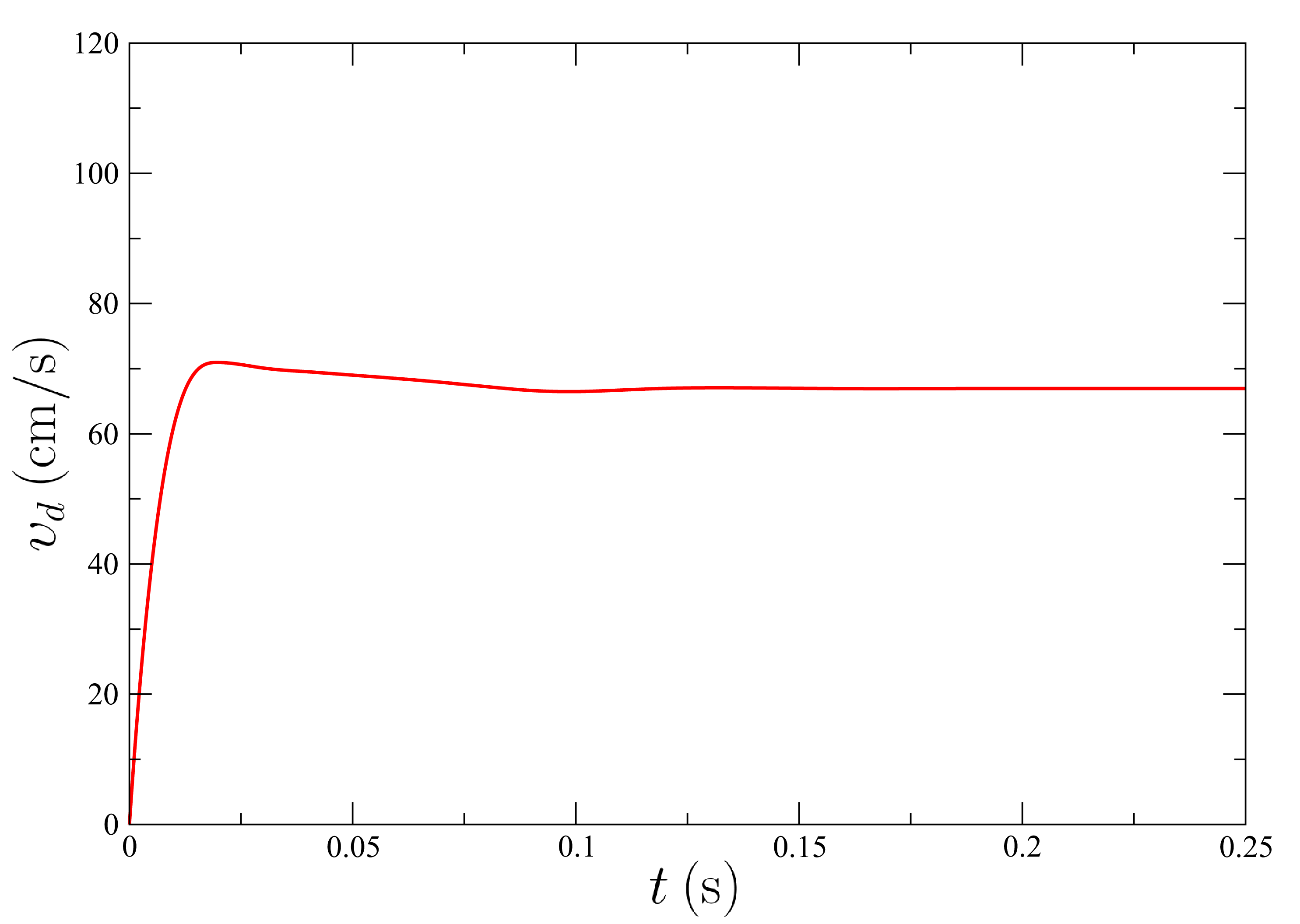
Figure 4: Time evolution of the drag velocity $\upsilon_{d}$. After an initial drift the $\upsilon_{d}$ value reaches a stationary regime with minimal fluctuations around a mean value.

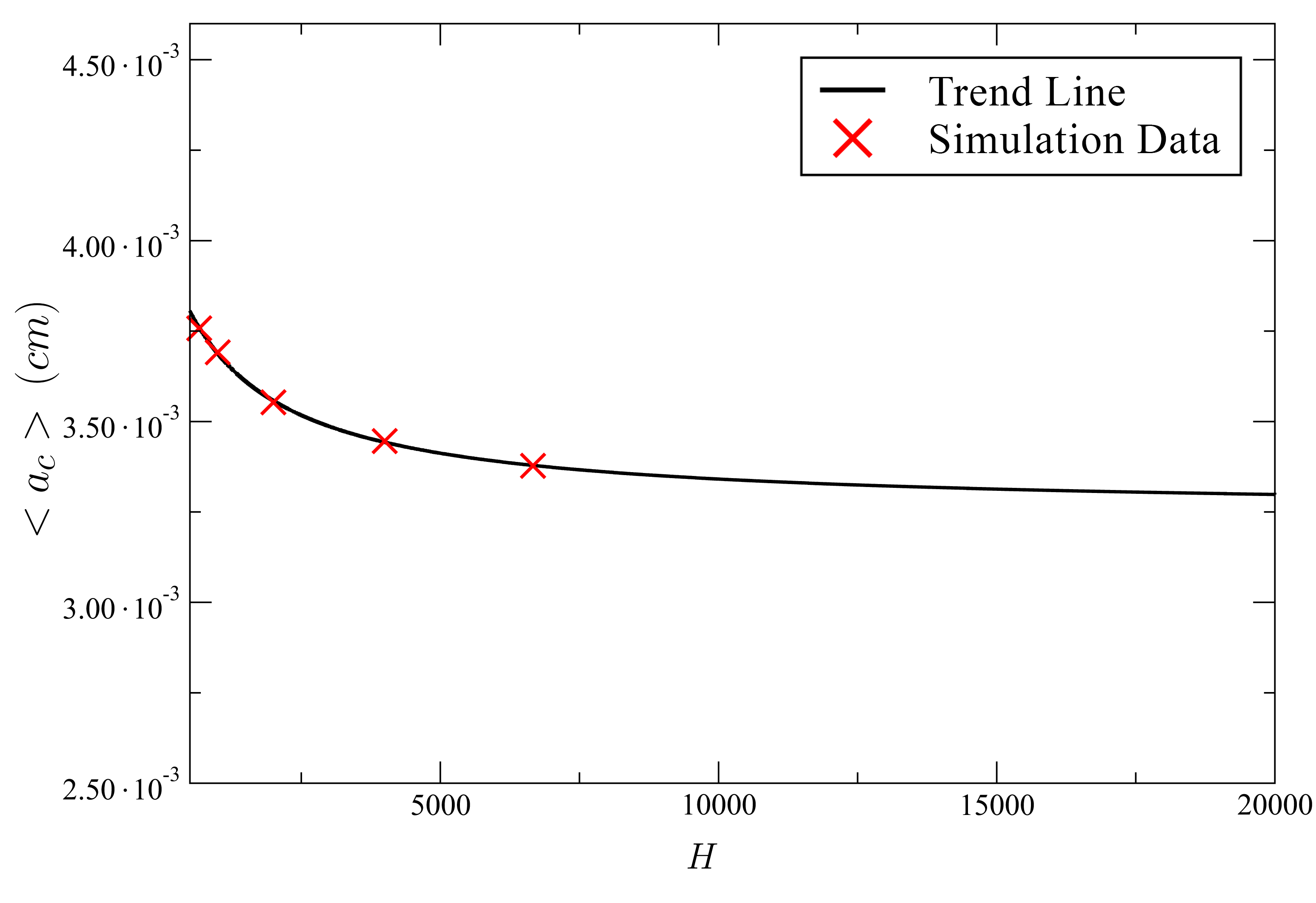
Figure 5: Averaged cross section radius $<a_{c}>$ of jet measured at the collector as function of the dimensionless parameter $H\propto 1/l_{step}$, which increases by decreasing $l_{step}$. A trend line is drawn to guide the reader’s eye and highlight the asymptotic behavior. It is worth stressing that the radius reduction ratio of the jet is here equal to only one order of magnitude, since in the 1-D model the bending instabilities are neglected and, therefore, the jet path is considerably shorter than in the corresponding 3-D simulation.

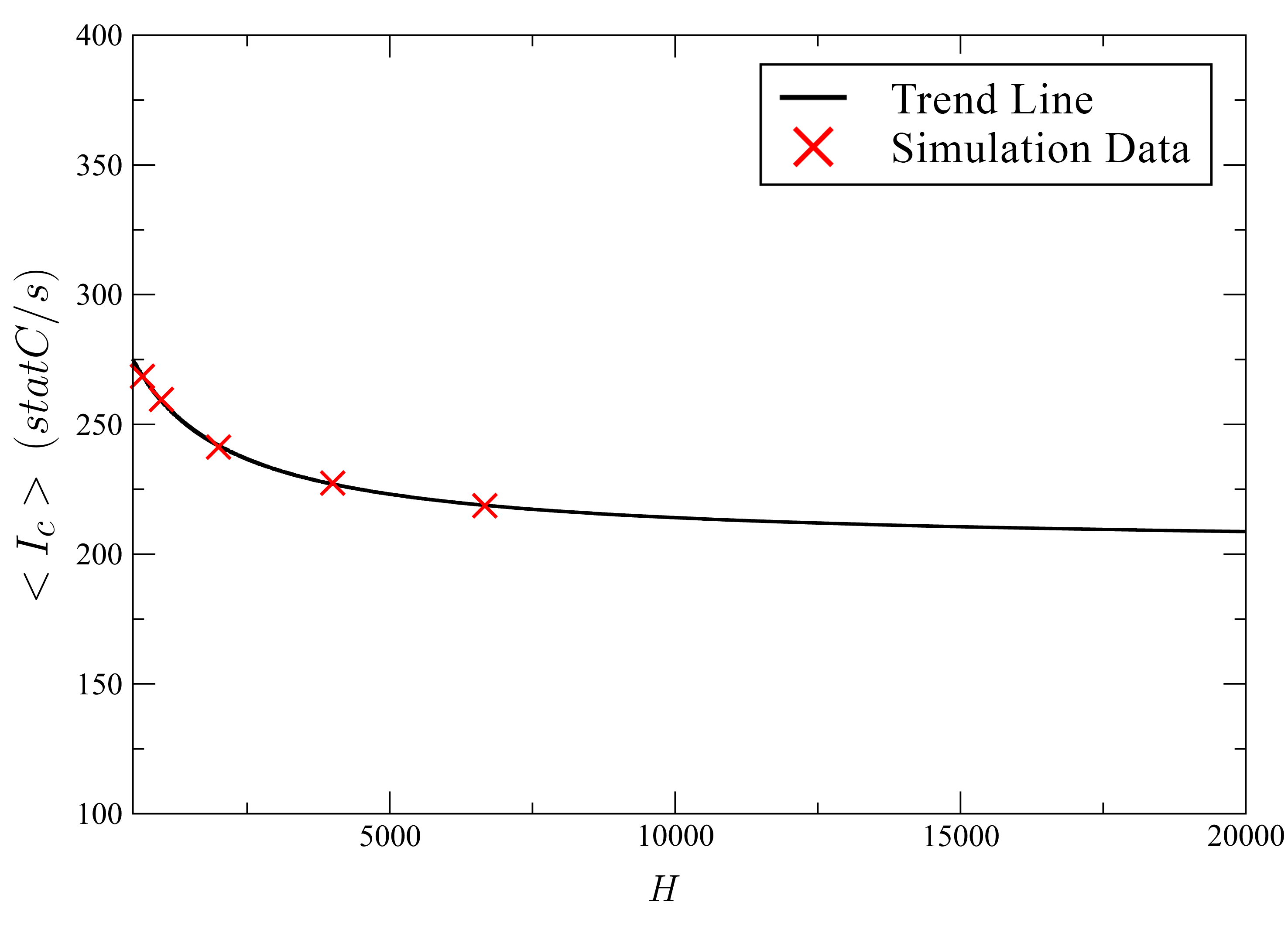
Figure 6: Averaged current $<I_{c}>$ measured at the collector as function of the dimensionless parameter $H\propto 1/l_{step}$, which increases by decreasing $l_{step}$. A trend line is drawn to guide the reader’s eye and highlight the asymptotic behavior.

Here, we run the input example labeled input 2 with different values of length step $l_{step}$. In particular, we probe the interval of $l_{step}$ values from $0.05$ to $0.3\text{cm}$. All the simulations started with the initial conditions $x=l_{step}$, $\sigma=0$, and $\upsilon_{x}=0$, and we integrated the EOM for 2 seconds. In all the simulations we observed an initial drift of the observables describing the electrospinning process. This drift occurs in the early stage of dynamics, when the jet has not reached the collector yet. After the jet touches the collector, the observables fluctuate around a constant mean value, providing a stationary regime. As example, we report in Fig4 the time evolution of the dragging velocity term $\upsilon_{d}$. Note that here $\upsilon_{d}$ is not equal to zero as in the previous case, since we have activated the injection of new beads by the directive inserting yes in the input file. In Fig5 and Fig6 we report the trend of two observables, average fiber radius and current measured at the collector in stationary regime, as function of the dimensionless parameter $H\propto 1/l_{step}$, which increases by decreasing $l_{step}$ (see Tab2 and Eq 12). In particular, we observe a slow asymptotic behavior of the two statistical data. Further discussions on the asymptotic behavior can be found in Refs [11, 34, 31]. It is worth stressing that the computational cost increases rapidly by decreasing $l_{step}$, and, therefore, the user should cleverly tune the length step $l_{step}$ in order to achieve a good compromise between efficiency and accuracy.

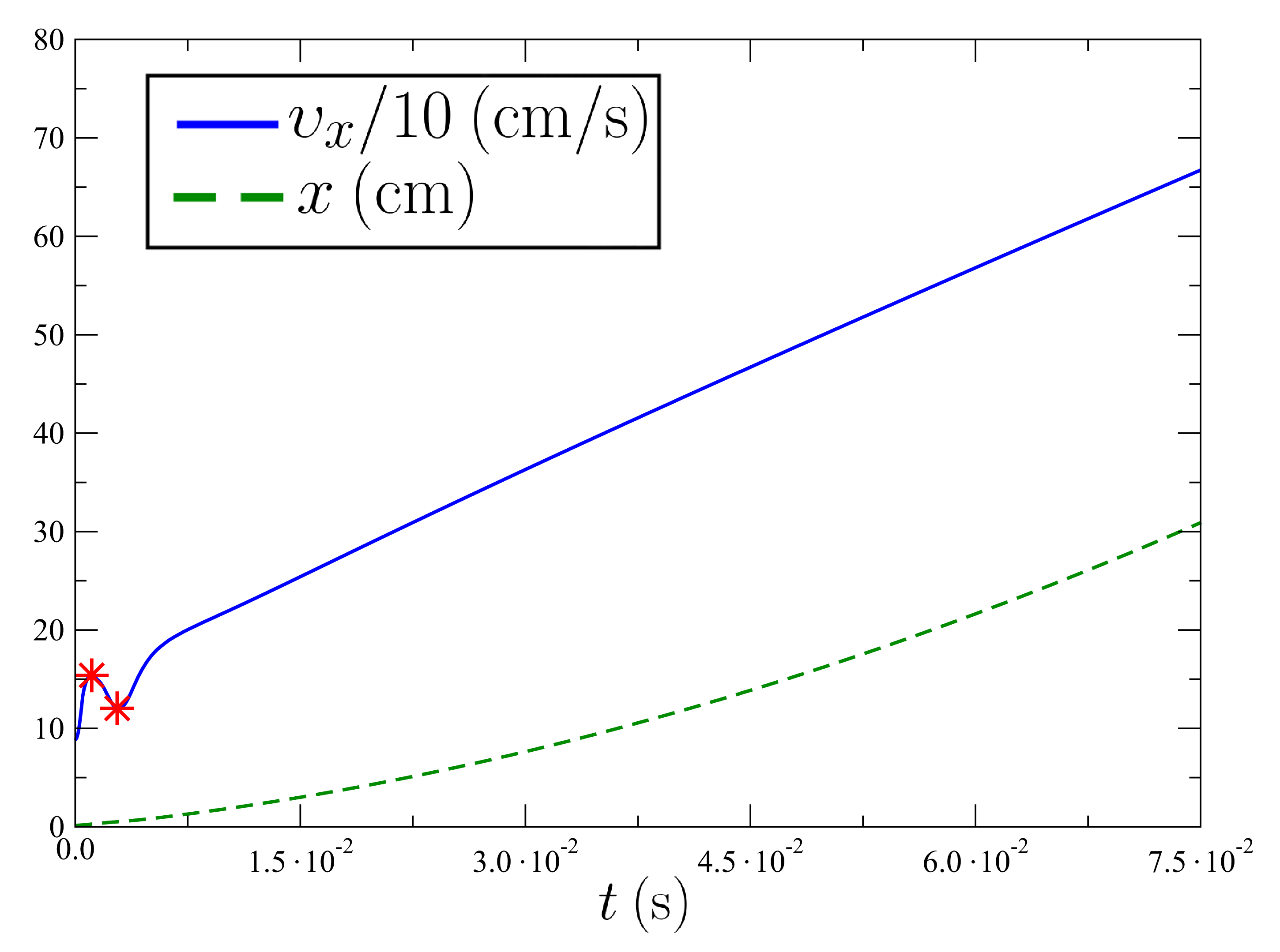
Figure 7: Time evolution of the velocity $\upsilon_{x}$ rescaled by a factor 1/10 (continuous line) and the length $x$ (dashed line). Two stages of the elongation process are observed. The first stage is biased by the sum of viscoelastic and Coulomb forces, and shows two quasi stationary points (denoted by red star symbols). Then, in the second stage the velocity comes to a near linearly increasing regime under the effect of the external electric field.

We report in Fig7 the time evolution of the position $x$ and velocity $\upsilon_{x}$ for a generic jet segment (jet bead) falling from the nozzle in stationary regime. Similarly to the previous case, we identify two sequential stages in the elongation process: the first biased by the sum of the viscoelastic and Coulomb forces, and the second dominated by the external electric field. Here the main difference compared to the previous case is the presence of two quasi stationary points instead of one. This fact is due to the larger viscoelastic force exerted by the new jet segments (beads) inserted at the nozzle. In fact, the viscoelastic force has a braking effect between the two quasi stationary points. Furthermore, comparing with the previous case we observe here that the presence of a non zero dragging velocity term $\upsilon_{d}$ anticipates the second stage.

7.3 Three-D simulations of a process leading to polymer nanofibers

The electrospinning of polyvinylpyrrolidone (PVP) nanofibers is a prototypical process, which has been largely investigated in literature.[6, 8, 5] Recently, its process dynamics was experimentally probed at an ultra-high time rate resolution by Montinaro et al.[37] Here, we simulate the electrospinning process of PVP solutions. Then, the theoretical results predicted by the models are compared with the aforementioned experimental data. In particular, we reproduce an experiment in which a solution of PVP (molecular weight = 1300 kDa) is prepared by a mixture of ethanol and water (17:3 v:v), at a concentration of about 2.5 wt%. The applied voltage is in a range around 10 kV, and the collector is placed at distance 16 cm from the nozzle, which has radius $250\,$micron (further details are provided in Ref. [37] ). As rheological properties of such system we consider the zero-shear viscosity $\mu_{0}=0.2\,\text{g}/(\text{cm}\cdot\text{s})$ [38, 39], the elastic modulus $G=5\cdot 10^{4}\,\text{g}/(\text{cm}\cdot\text{s}^{2})$ [40], and the surface tension $\alpha=21.1\,\text{g}/\text{s}^{2}$ [38]. We use for the simulation a viscosity value $\mu$ which is two order of magnitude larger than the zero-shear viscosity $\mu_{0}$ reported, since the strong longitudinal flows we are dealing with can lead to an increase of the extensional viscosity from $\mu_{0}$, as already observed in literature.[11, 41] The mass density is equal to $0.84\,\text{g}/\text{cm}^{3}$, while the charge density was estimated by experimental observations of the current measured at the nozzle. For convenience, all the simulation parameters are summarized in Tab3.

We show here the results three independent simulations with different values of potential $V_{0}$ between the nozzle and the collector: 6 kV, 9 kV and 11 kV, respectively. The simulations were carried out with a time step of $10^{-7}$ s, the EOM were integrated in time for 20 million steps by using the second order accurate Heun scheme. As example, one of the three input files is reported as labeled input 3. Note that we have activated the perturbation module by the directive perturb yes in the input file, in order to model a mechanical perturbation at the nozzle. Here, we use the frequency of the perturbation value $\omega$ proposed by Reneker et al.[11]

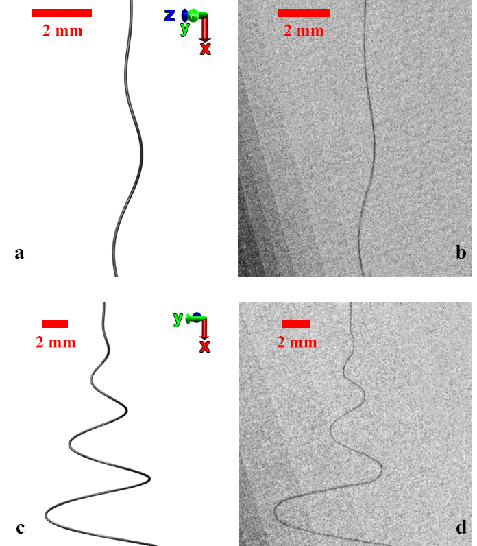
Figure 8: Snapshots of the simulated jet (a,c) and of the experimental jet (b,d) taken close the nozzle in the early stage (a,b), and in the bending regime (c,d) of dynamics.

In all the simulations, we recognize three different stages of the electrospun jet: 1) extensione along a straight line over a few centimeters, 2) slight perturbation from the linear path leading to bending instability; 3) fully three-dimensional motion out from the stretching axis. Two snapshots of the simulated jet are reported on the left of Fig8, which can be compared with two high-frame-rate micrographs (on the right of the figure) collected during electrospinning experiments [37]. The two shown snapshots correspond to an early stage and a later regime of instabilities, respectively. We note a general good agreement between the simulation results and experimental measurements. Furthermore, we monitored the velocity of the jet ejected at the nozzle, whose value was estimated between $2.0$ and $2.4$ m/s for the case $V_{0}=9$kV. This is also pretty close to the experimental observations which locate the velocity around 2.6 m/s [37].

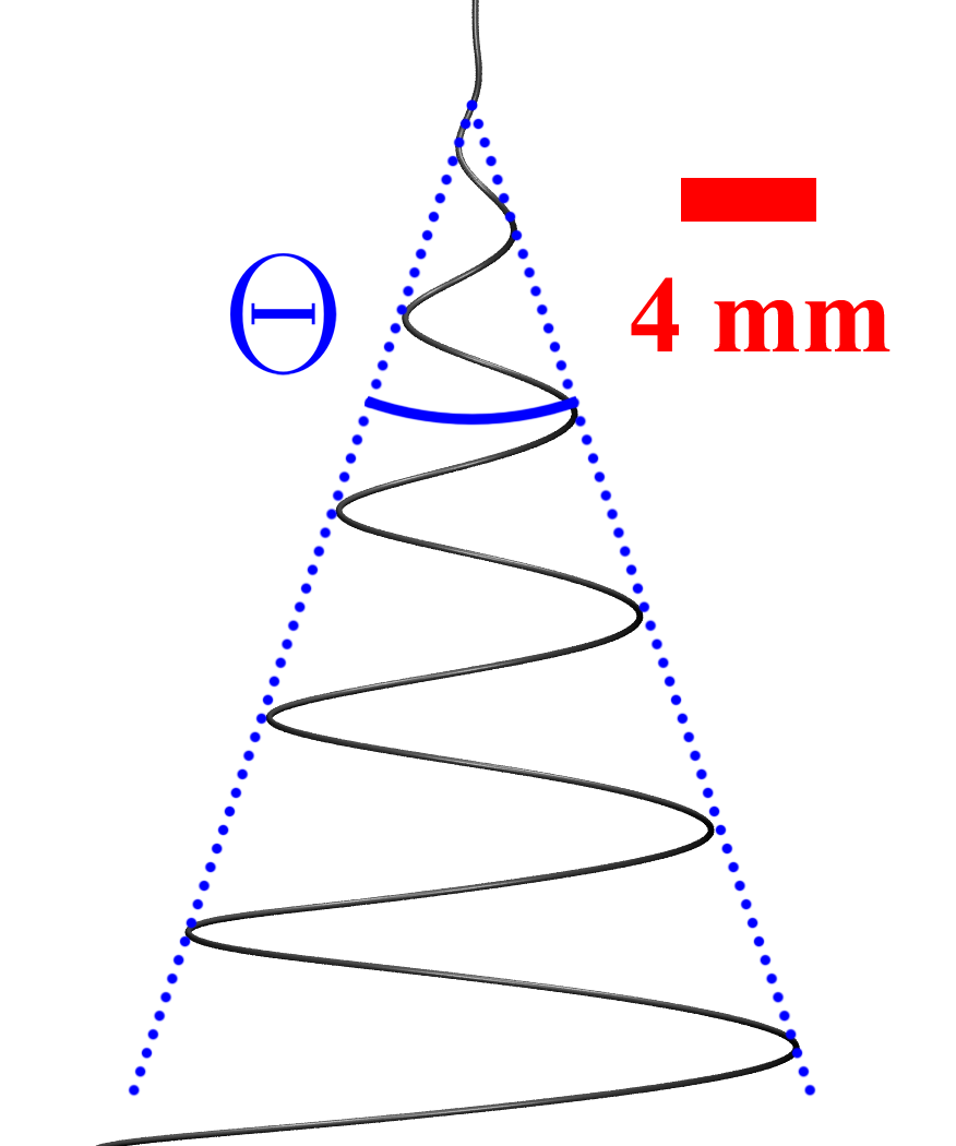
Figure 9: Snapshot showing the instability broadening in stationary regime and highlighting the resulting angular aperture $\Theta$.

As mentioned above, bending instabilities play an important role in the electrospinning process, since they increase the path traveled by the jet from the nozzle to the collector with beneficial effect in terms of yielding a smaller polymer fiber radius. Thus, we measure the instantaneous angular aperture ($\Theta$) of the instability cone (see Fig9) in the range of potential $V_{0}$ imposed between the nozzle and the collector (from 6 up to 11 V). The $\Theta$ values are in the range 30-36 degrees, which is consistent with the experimentally measured range 29-37 degrees reported in Ref [37].

8 Performance

The performance of the underlying numerical routines in JETSPIN is an important aspect to take into account, affecting the choice of the value of the discretization length step allowing the jet to be discretised without loosing accuracy. In simulating electrospinning processes, this factor is especially important given that upon decreasing the discretization length step the systems size (number of beads) increases with linear dependence. Furthermore, the code currently spends of order $N^{2}$ operations to compute the Coulomb force ($N$ is the number of beads). The last point could be addressed in future versions of the code by using strategies like linked cell or tree-code algorithm.

In this Section, we compare the CPU wall-clock time required to run the input 1 and input 3 with the three different integration schemes implemented in JETSPIN. For the input 1 case, we note that the increase of CPU wall-clock time is strongly dependent on the greater complexity of the chosen integrator scheme (see Tab4). In particular, we note that the Heun and Runge-Kutta schemes require around two and four times the CPU wall-clock time cost of the Euler integrator, respectively. A similar trend is observed also for the input 3 case. However, the user should also consider the different numerical accuracy provided by the three schemes, as already discussed in Subsec 7.1.

We probe the parallel efficiency of JETSPIN. In particular, we run the input 3 at different values of discretization length step and collector-nozzle distance. Thus, we probe different system sizes corresponding to different numbers of beads, which are used to discretise the jet. Further, the procedure is repeated with different number of processing cores, so that the efficiency of the implemented parallel strategy is investigated. In order to perform a quantitative analysis, we compute the speedup ($S_{p}$)

$$S_{p}=\frac{T_{s}}{T_{p}},$$ (16)

where $T_{s}$ stands for the CPU wall-clock time of the code in serial mode, and $T_{p}$ the CPU wall-clock time of the code in parallel mode executed by the number of processors denoted $n_{p}$.

We also estimate the parallel efficiency ($E_{p}$) defined as

$$E_{p}=\frac{S_{p}}{n_{p}}.$$ (17)

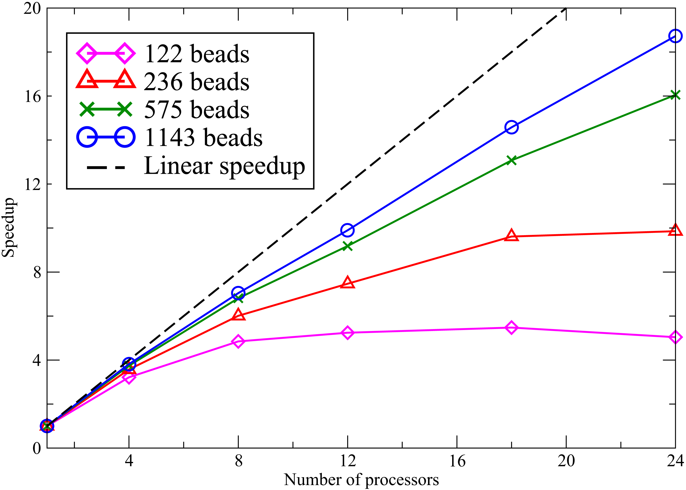
Figure 10: Speedup versus number of processors for different system sizes. Ideally, the speedup should be equal to the number of processors (linear speedup in black dashed line).

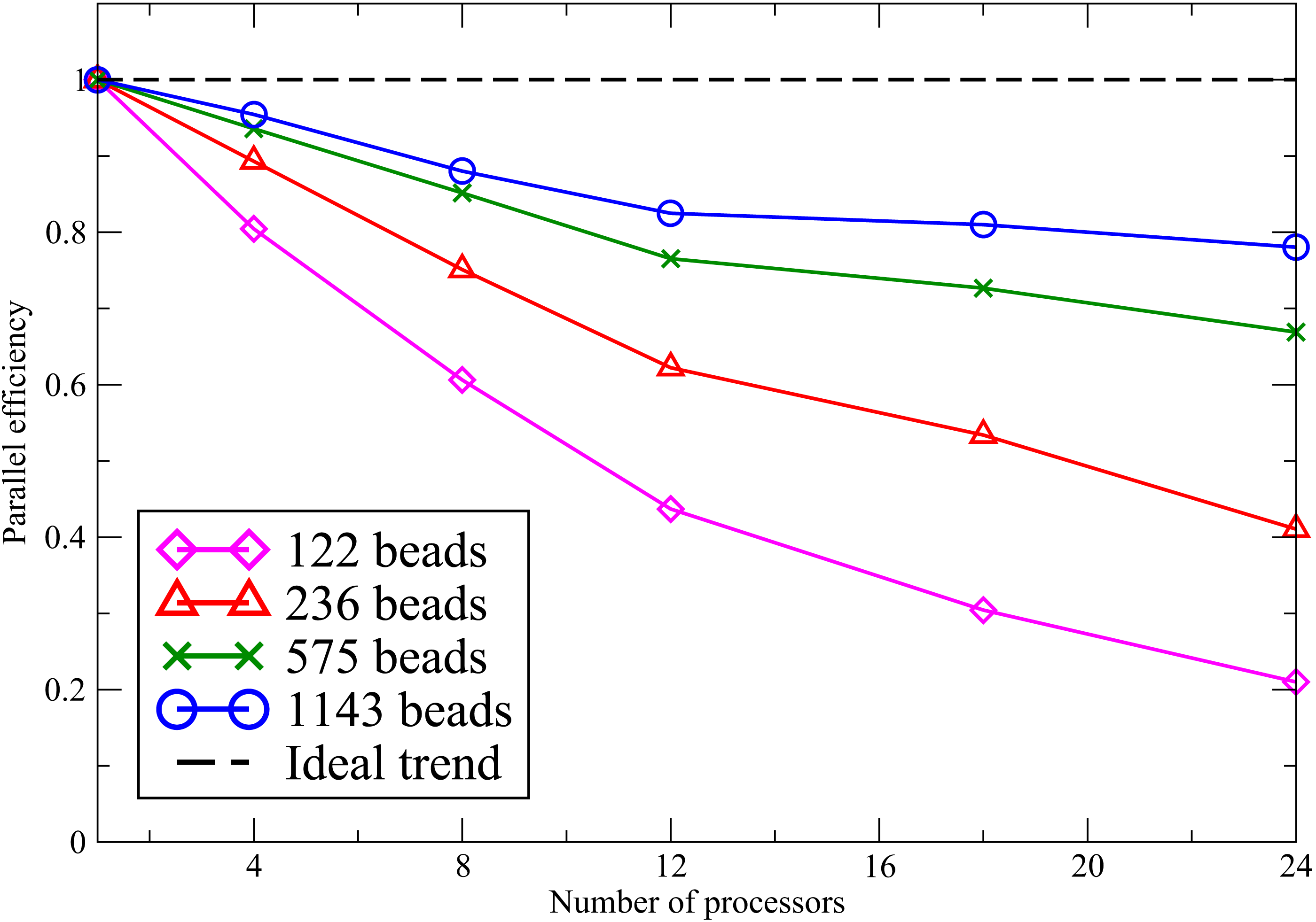
Figure 11: Parallel efficiency versus number of processors for different system sizes. Note that we observe a parallel efficiency larger than 0.8 only if the system size provides at least 50 beads per each processor. We report the ideal parallel efficiency in black dashed line which should be equal to one for any number of processors.

The trends of these two estimators versus the number of processors are reported in Fig10 and Fig11. Note that only for the largest system size we observe a quasi linear trend of $S_{p}$ (see Fig10), while in all the other cases a sub-linear behavior is evident (note that the speedup should ideally be equal to the number of processors). This is not surprising, since the communication latency strays actually the speedup from the linear trend. Note that deviation from the linear trend is larger for smaller system sizes with a lower cost-benefit ratio. This is usually due to the communication latency which deteriorates the performance whenever the number of beads assigned to each processor is not sufficiently high to offset the communication overheads. This is evident in Fig11, where the parallel efficiency is usually larger than 0.8 (80%) only if the system size provides at least 50 beads per each processor. As a consequence, the user should always consider the number of beads handled by each processor in order to run efficiently JETSPIN in parallel mode.

9 Availability

JETSPIN is available free under the Open Software License v. 3.0 (OSL) created by Lawrence Rosen[42]. However, it is worth stressing that all commercial rights derived from this software are entirely owned by the authors as reported in paragraph 4 of the OSL. A copy of the code may be obtained as zipped and tarred file at the website: http://www.nanojets.eu/. All enquiries regarding how to obtain a copy of JETSPIN should be addressed to the authors.

10 Conclusions

We have presented JETSPIN, a new open-source software for the numerical simulation of electrospinning phenomena. JETSPIN is implemented in FORTRAN programming language and permits to simulate a wide spectrum of structured polymer fibers with diameters in the range from several micrometers down to tens of nanometers, which are of considerable interest for various applications. In this work, we have described the basic structure of the code and the main features of the implemented model. In addition, we have discussed a number of examples intended to convey the reader a flavor of the type of problems which are suitable for JETPSIN simulation. In particular, the simulations of prototypical polymer materials demonstrate the capabilities of the present code to reproduce experimental data.

JETSPIN is expevcted to provide a useful tool to investigate relationships among the relevant process variables, material parameters and experimental settings, and to predict the dynamics and the characteristics of the jet, many of which can be found in resulting collected nanofibers. Further, it can be used to identify the role played by the concurrent physical mechanism participating to the electrospinning process. In summary, JETSPIN can complement and support experiments with the aim of enhancing the efficiency of the electrospinning process and the quality of electrospun fiber materials.

Appendix A

directive:	meaning:
collector distance $f$	distance of collector from the nozzle along the x axis
	(note the nozzle is assumed in the origin)
cutoff $f$	length of the proximal jet sections interacting by Coulomb
	force (default: equal to the collector distance)
density mass $f$	mass density of the jet
density charge $f$	electric volume charge density of the jet
elastic modulus $f$	elastic modulus of the jet
external potential $f$	electric potential between the nozzle and collector
final time $f$	set the end time of the simulation
finish	close the input file (last data record)
gravity yes	activate the inclusion of the gravity force in the model
initial length $f$	length of the jet at the initial time
integrator $i$	set the integration scheme. The integer can be ’1’ for
	Euler, ’2’ for Heun, and ’3’ for Runge-Kutta scheme
inserting yes	inject new beads as explained in Subsec 4.3
nozzle cross $f$	cross section radius of the jet at the nozzle
nozzle stress $f$	viscoelastic stress of the jet at the nozzle
nozzle velocity $f$	bulk fluid velocity of the jet at the nozzle
perturb yes	activate the periodic perturbation at the nozzle
perturb freq $f$	frequency of the perturbation at the nozzle
perturb ampl $f$	amplitude of the perturbation at the nozzle
points $i$	number of segment in which the jet is discretised
print list $s_{1}\,\ldots$	print on terminal statistical data as indicated by symbolic
	strings (see Appendix B for detailed informations)
print time $f$	print data on terminal and output file every $f$ seconds
print xyz $f$	print the trajectory in XYZ file format in centimeters
	every $f$ seconds
print xyz maxnum $i$	print the XYZ file format with $i$ beads starting from the
	nearest bead to the collector (default: 100)
print xyz rescale $f$	print the XYZ file format data rescaled by $f$
printstat list $s_{1}\,\ldots$	print on output file statistical data as indicated by symbolic
	strings (see Appendix B for detailed informations)
removing yes	remove beads at collector
resolution $f$	discretization step length of the jet
surface tension $f$	surface tension coefficient of the jet
system $i$	set the jet model. The integer can be equal to
	’1’ for select the 1d-model or ’3’ for the 3d-model
timestep $f$	set the time step for the integration scheme
viscosity $f$	viscosity of the jet

Here, we report the list of directives available in JETSPIN. Note $i$, $f$, and $s$ denote an integer number, a floating point number, and a string, respectively. The underlined directives are mandatory. The default value is zero (exceptions are stressed in parentheses).

Appendix B

keys:	meaning:
t	unscaled time
ts	scaled time
x, y, z	unscaled coordinates of the farest bead
xs, ys, zs	scaled coordinates of the farest bead
st	unscaled stress of the farest bead
sts	scaled stress of the farest bead
vx, vy, vz	unscaled velocities of the farest bead
vxs, vys, vzs	scaled velocities of the farest bead
yz	unscaled normal distance from the x axis of the farest bead
yzs	scaled normal distance from the x axis of the farest bead
mass	last inserted mass at the nozzle
q	last inserted charge at the nozzle
cpu	time for every print interval
cpur	remaining time to the end
cpue	elapsed time
n	number of beads used to discretise the jet
f	index of the first bead
l	index of the last bead
curn	current at the nozzle
curc	current at the collector
vn	velocity modulus of jet at the nozzle
vc	velocity modulus of jet at the collector
svc	strain velocity at the collector
mfn	mass flux at the nozzle
mfc	mass flux at the collector
rc	radius of jet at the collector
rrr	radius reduction ratio of jet
lp	length path of jet
rlp	length path of jet divided by the collector distance

In JETSPIN a series of instantaneous and statistical data are available to be printed by selecting the appropriate key. Here, the list of symbolic string keys is reported with their corresponding meanings. Note that by scaled we mean that the observable was rescaled by the characteristic values provided in Tab2. The underlined keys correspond to data which are averaged on the time interval given by the directive print time in input file. By farest bead we mean the farest bead from the nozzle (with greatest $x$ value). All the quantities are expressed in centimeter–gram–second unit system, excepted the dimensionless scaled observables.

Tables

target:	meaning:
gfortran	compile in serial mode using the GFortran compiler.
gfortran-mpi	compile in parallel mode using the GFortran compiler and the Open Mpi library.
cygwin	compile in serial mode using the GFortran compiler under the command-line
	interface Cygwin for Windows.
cygwin-mpi	compile in parallel mode using the GFortran compiler and the Open Mpi library
	under the command-line interface Cygwin for Windows (note a precompiled
	package of the Open Mpi library is already available on Cygwin).
intel	compile in serial mode using the Intel compiler.
intel-mpi	compile in parallel mode using the Intel compiler and the Intel Mpi library.
intel-openmpi	compile in parallel mode using the Intel compiler and the Open Mpi library.
help	return the list of possible target choices

Table 1: List of targets for several common workstations and parallel computers, which can be used by the command "make target".

Characteristic Scales
$L_{0}=l_{step}\sqrt{\frac{\pi a_{0}^{2}\rho_{V}^{2}}{G}}$	$t_{0}=\frac{\mu}{G}$
$\sigma_{0}=G$
Dimensionless Derived Variables
$\bar{l}_{i}={\displaystyle\frac{l_{i}}{L_{0}}}$	$\bar{R}_{ij}={\displaystyle\frac{R_{ij}}{L_{0}}}$
$\bar{k}=kL_{0}$
Dimensionless Groups
$V_{i}={\displaystyle\frac{q_{i}V_{0}\mu^{2}}{m_{i}h\,L_{0}\,G^{2}}}$	$Q_{ij}={\displaystyle\frac{q_{i}q_{j}\mu^{2}}{L_{0}^{3}m_{i}G^{2}}}$
$F_{ve,i}={\displaystyle\frac{\pi a_{0}^{2}\mu^{2}}{m_{i}L_{0}G}}$	$A_{i}={\displaystyle\frac{\alpha\pi a_{0}^{2}\mu^{2}}{m_{i}L_{0}^{2}G^{2}}}$
$F_{g}={\displaystyle\frac{g\mu^{2}}{L_{0}G^{2}}}$	$K_{s}=\omega{\displaystyle\frac{\mu}{G}}$
$H={\displaystyle\frac{h}{L_{0}}}$	$L_{step}={\displaystyle\frac{l_{step}}{L_{0}}}$

Table 2: Definitions of the characteristic scales, dimensionless derived variables, and groups employed in the text.

$\rho$	$\rho_{q}$	$a_{0}$	$\upsilon_{s}$	$\alpha$	$\mu$	$G$	$V_{0}$	$\omega$	$A$
($\text{kg}/\text{m}^{3}$)	($\text{C}/\text{L}$)	(cm)	(cm/s)	(mN/m)	(Pa$\cdot$s)	(Pa)	(kV)	($\text{s}^{-1}$)	(cm)
840	$2.8\cdot 10^{-7}$	$5\cdot 10^{-3}$	0.28	21.1	2.0	50000	9.0	$10^{4}$	$10^{-3}$

Table 3: Simulation parameters for the simulation of PVP nanofibers. The headings used are as follows: $\rho$: density, $\rho_{q}$: charge density, $a_{0}$: fiber radius at the nozzle, $\upsilon_{s}$: bulk fluid velocity in the syringe needle, $\alpha$: surface tension, $\mu$: viscosity, $G$ : elastic modulus, $V_{0}$ : applied voltage bias, $\omega$: frequency of perturbation, $A$ : amplitude of perturbation. The bulk fluid velocity $\upsilon_{s}$ was estimated considering that the solution was pumped at constant flow rate of 2 mL/h in a needle of radius $250\,$micron.

Input file	Integrator scheme	# of CPUs	Parallel	CPU time (s)*	# of beads	CPU time (s)*
			efficiency			per bead and step
Input 1	Euler	1	-	4.76	1	$4.76\cdot 10^{-7}$
Input 1	Heun	1	-	8.64	1	$8.64\cdot 10^{-7}$
Input 1	Runge-Kutta	1	-	16.72	1	$16.72\cdot 10^{-7}$
Input 3	Euler	4	0.8	11307.47	150	$1.51\cdot 10^{-6}$
Input 3	Heun	4	0.8	22368.07	150	$2.98\cdot 10^{-6}$
Input 3	Runge-Kutta	4	0.8	44708.62	150	$5.96\cdot 10^{-6}$

Table 4: We report the CPU wall-clock time in seconds which is needed to run the input 1 and input 3 example files. For each of the two input files we test the three different integration schemes implemented in JETSPIN: the first-order accurate Euler scheme, the second-order accurate Heun scheme, and the fourth-order accurate Runge-Kutta scheme. *The benchmark of the input 1 was carried out on an Intel Core I5 480M (3M Cache, 2.66 GHz) in serial mode, while the input 3 benchmark was executed in parallel mode (4 CPUs) on a node of 2x12 core processors made of 2.4 GHz Intel Ivy Bridge cores. We report also the number of beads used to discretise the jet, and the CPU time which is needed to integrate one bead for one time step.

Input 1. Example JETSPIN input file for electrospinning simulation.
system 1
integrator 2
timestep 1.d-8
final time 1.d-1
print time 1.d-3
print list ts xs sts vxs cpu cpur cpu
printstat list ts xs sts vxs cpu cpur cpu
inserting no
removing no
points 1
initial length 3.19d-1
nozzle cross 1.5d-2
density mass 8.18912288d-1
density charge 3761.26389d0
viscosity 100.d0
elastic modulus 10000.d
collector distance 200.d0
external potential 277.8141d0
finish

Input 2. Example JETSPIN input file for electrospinning simulation.
system 1
integrator 3
timestep 1.d-7
final time 2.d0
print time 1.d-2
print list t x cpu cpur n rc curc
printstat list t x st vx cpu cpue cpur n rc curc vc mfc
inserting yes
removing yes
points 1
initial length 0.10d0
nozzle cross 1.5d-2
density mass 8.1991d-1
density charge 37607.35d0
viscosity 100.d0
elastic modulus 10000.d
collector distance 200.d0
external potential 277.8141d0
finish

Input 3. Example JETSPIN input file for electrospinning simulation.
system 3
integrator 2
timestep 1.d-8
final time 0.5d0
print time 1.d-2
print list t x vn vc yz n curn curc
printstat list t x vn vc yz n curn curc
print xyz 1.d-4
print xyz maxnumber 400
inserting yes
removing yes
gravity yes
points 1
initial length 0.02.d0
nozzle cross 5.d-3
density mass 0.84d0
density charge 44000.d0
viscosity 20.d0
elastic modulus 50000.d0
collector distance 16.d0
external potential 30.02d0
surface tension 21.13d0
perturbation yes
perturbation frequency 1.d+4
perturbation amplitude 1.d-3
finish

Figures

References

- [1] D. Li, Y. Wang, Y. Xia, Electrospinning nanofibers as uniaxially aligned arrays and layer-by-layer stacked films, Advanced Materials 16 (4) (2004) 361–366.
- [2] A. Greiner, J. H. Wendorff, Electrospinning: a fascinating method for the preparation of ultrathin fibers, Angewandte Chemie International Edition 46 (30) (2007) 5670–5703.
- [3] C. P. Carroll, E. Zhmayev, V. Kalra, Y. L. Joo, Nanofibers from electrically driven viscoelastic jets: modeling and experiments, Korea-Aust Rheol J 20 (2008) 153–164.
- [4] Z.-M. Huang, Y.-Z. Zhang, M. Kotaki, S. Ramakrishna, A review on polymer nanofibers by electrospinning and their applications in nanocomposites, Composites science and technology 63 (15) (2003) 2223–2253.
- [5] L. Persano, A. Camposeo, C. Tekmen, D. Pisignano, Industrial upscaling of electrospinning and applications of polymer nanofibers: a review, Macromolecular Materials and Engineering 298 (5) (2013) 504–520.
- [6] A. L. Yarin, B. Pourdeyhimi, S. Ramakrishna, Fundamentals and Applications of Micro and Nanofibers, Cambridge University Press, 2014.
- [7] J. H. Wendorff, S. Agarwal, A. Greiner, Electrospinning: materials, processing, and applications, John Wiley & Sons, 2012.
- [8] D. Pisignano, Polymer Nanofibers: Building Blocks for Nanotechnology, Royal Society of Chemistry, 2013.
- [9] Y. Zeng, Y. Wu, Z. Pei, C. Yu, Numerical approach to electrospinning, International Journal of Nonlinear Sciences and Numerical Simulation 7 (4) (2006) 385–388.
- [10] J. Feng, Stretching of a straight electrically charged viscoelastic jet, Journal of Non-Newtonian Fluid Mechanics 116 (1) (2003) 55–70.
- [11] D. H. Reneker, A. L. Yarin, H. Fong, S. Koombhongse, Bending instability of electrically charged liquid jets of polymer solutions in electrospinning, Journal of Applied physics 87 (9) (2000) 4531–4547.
- [12] A. L. Yarin, S. Koombhongse, D. H. Reneker, Taylor cone and jetting from liquid droplets in electrospinning of nanofibers, Journal of Applied Physics 90 (9) (2001) 4836–4846.
- [13] S. V. Fridrikh, H. Y. Jian, M. P. Brenner, G. C. Rutledge, Controlling the fiber diameter during electrospinning, Physical review letters 90 (14) (2003) 144502.
- [14] S. Theron, E. Zussman, A. Yarin, Experimental investigation of the governing parameters in the electrospinning of polymer solutions, Polymer 45 (6) (2004) 2017–2030.
- [15] C. Lu, P. Chen, J. Li, Y. Zhang, Computer simulation of electrospinning. part i. effect of solvent in electrospinning, Polymer 47 (3) (2006) 915–921.
- [16] X. Wang, Y. Liu, C. Zhang, Y. An, X. He, W. Yang, Simulation on electrical field distribution and fiber falls in melt electrospinning, Journal of nanoscience and nanotechnology 13 (7) (2013) 4680–4685.
- [17] I. Coluzza, D. Pisignano, D. Gentili, G. Pontrelli, S. Succi, Ultrathin fibers from electrospinning experiments under driven fast-oscillating perturbations, Physical Review Applied 2 (5) (2014) 054011.
- [18] G. Pontrelli, D. Gentili, I. Coluzza, D. Pisignano, S. Succi, Effects of non-linear rheology on the electrospinning process: a model study, Mechanics Research Communications 61 (2014) 41–46.
- [19] M. Lauricella, G. Pontrelli, I. Coluzza, D. Pisignano, S. Succi, Different regimes of the uniaxial elongation of electrically charged viscoelastic jets due to dissipative air drag, Submitted to Mech. Res. Comm., (2014).
- [20] M. Lauricella, G. Pontrelli, D. Pisignano, S. Succi, Non-linear langevin model for the early-stage dynamics of electrospinning jets, Submitted to Molecular Physics, (2015).
- [21] J. Racine, The cygwin tools: a gnu toolkit for windows, Journal of Applied Econometrics 15 (3) (2000) 331–341.
- [22] W. Smith, Molecular dynamics on hypercube parallel computers, Computer Physics Communications 62 (2) (1991) 229–248.
- [23] D. Brown, J. H. Clarke, M. Okuda, T. Yamazaki, A domain decomposition parallelization strategy for molecular dynamics simulations on distributed memory machines, Computer Physics Communications 74 (1) (1993) 67–80.
- [24] A. Yarin, S. Koombhongse, D. H. Reneker, Bending instability in electrospinning of nanofibers, Journal of Applied Physics 89 (5) (2001) 3018–3026.
- [25] T. A. Kowalewski, S. Barral, T. Kowalczyk, Modeling electrospinning of nanofibers, in: IUTAM symposium on modelling nanomaterials and nanosystems, Springer, 2009, pp. 279–292.
- [26] S. M. Hanasoge, S. Succi, S. A. Orszag, Lattice boltzmann method for electromagnetic wave propagation, EPL (Europhysics Letters) 96 (1) (2011) 14002.
- [27] R. Benzi, S. Succi, M. Vergassola, The lattice boltzmann equation: theory and applications, Physics Reports 222 (3) (1992) 145–197.
- [28] M. Ottaviani, F. Romanelli, R. Benzi, M. Briscolini, P. Santangelo, S. Succi, Numerical simulations of ion temperature gradient-driven turbulence, Physics of Fluids B (1989-1993) 2 (1) (1990) 67–74.
- [29] J. Feng, The stretching of an electrified non-newtonian jet: A model for electrospinning, Physics of Fluids (1994-present) 14 (11) (2002) 3912–3926.
- [30] M. M. Hohman, M. Shin, G. Rutledge, M. P. Brenner, Electrospinning and electrically forced jets. i. stability theory, Physics of Fluids (1994-present) 13 (8) (2001) 2201–2220.
- [31] T. Kowalewski, S. NSKI, S. Barral, Experiments and modelling of electrospinning process, Technical Sciences 53 (4).
- [32] A. Ziabicki, H. Kawai, High-Speed Fiber Spinning: Science and Engineering Aspects, Krieger Publishing Co, 1991.
- [33] W. H. Press, Numerical recipes 3rd edition: The art of scientific computing, Cambridge university press, 2007.
- [34] C. P. Carroll, Y. L. Joo, Discretized modeling of electrically driven viscoelastic jets in the initial stage of electrospinning, Journal of Applied Physics 109 (9) (2011) 094315.
- [35] W. Humphrey, A. Dalke, K. Schulten, Vmd: visual molecular dynamics, Journal of molecular graphics 14 (1) (1996) 33–38.
- [36] E. F. Pettersen, T. D. Goddard, C. C. Huang, G. S. Couch, D. M. Greenblatt, E. C. Meng, T. E. Ferrin, Ucsf chimera: a visualization system for exploratory research and analysis, Journal of computational chemistry 25 (13) (2004) 1605–1612.
- [37] M. Montinaro, V. Fasano, M. Moffa, A. Camposeo, L. Persano, M. Lauricella, S. Succi, D. Pisignano, Sub-ms dynamics of the instability onset of electrospinning, Submitted to Soft Matter.
- [38] N. Yuya, W. Kai, B.-S. Kim, I. Kim, Morphology controlled electrospun poly(vinyl pyrrolidone) fibers: effects of organic solvent and relative humidity, Journal of Materials Science and Engineering with Advanced Technology.
- [39] V. Bühler, Polyvinylpyrrolidone excipients for pharmaceuticals: povidone, crospovidone and copovidone, Springer Science & Business Media, 2005.
- [40] V. N. Morozov, A. Y. Mikheev, Water-soluble polyvinylpyrrolidone nanofilters manufactured by electrospray-neutralization technique, Journal of Membrane Science 403 (2012) 110–120.
- [41] A. L. Yarin, Free liquid jets and films: hydrodynamics and rheology, Longman Scientific & Technical Harlow, 1993.
-
[42]
L. Rosen, The open software
license 3.0 (2005).
URL http://opensource.org/licenses/OSL-3.0/