Non-Abelian T-duality for nonrelativistic holographic duals

Thiago R. Araujo^a, and Horatiu Nastase^a,

^a Instituto de Física Teórica, UNESP-Universidade Estadual Paulista

R. Dr. Bento T. Ferraz 271, Bl. II, Sao Paulo 01140-070, SP, Brazil

Abstract

We find new type II backgrounds with non-relativistic symmetries via non-Abelian T-duality. First we consider geometries with Galilean symmetries in type IIA, which have been identified as non-relativistic generalizations of the ABJM background and massive IIA supergravities. We then consider the non-Abelian T-duality transformation on the backgrounds with Lifshitz symmetry constructed by Donos and Gauntlett. Using gauge/gravity duality we study aspects of the field theory dual to these backgrounds.

1 Introduction

Gauge/gravity duality [1, 2, 3] (for a standard review, see [4]) has had a lot of success describing gauge theories, when derived from the decoupling limit of a system of branes.

But a lot of the recent interest has been instead focused on applications to condensed matter physics, specifically in the study of strongly coupled systems described by relativistic and also nonrelativistic field theories. Since gauge/gravity duality relates strong coupling in field theory to weak coupling in gravity (and vice versa), we can analyze models that are otherwise very difficult to analyze. Since however in these AdS/CMT cases we usually have no decoupled system of branes, only a phenomenological construction of a gravity dual, we have usually less control over the construction. One degree of control is obtained by analyzing symmetry.

The symmetries of the field theory are realized geometrically as isometries in the gravity dual side. In the best known example, type IIB string theory on $AdS_{5}\times S^{5}$ vs. ${\cal N}=4$ SYM, the isometry group of the gravity dual is $SO(4,2)\times SO(6)$, matching with the one of a four dimensional conformal field theory with ${\cal N}=4$ supersymmetries [1]. While the $SO(4,2)$ symmetry of the anti-de Sitter space is reinterpreted as the conformal group in $3+1$ dimensions, the group $SO(6)\simeq SU(4)$ can be identified with the R-symmetry group of the conformal theory.

In the case of strongly coupled condensed matter systems, we have a variety of numerical and theoretical tools from statistical physics and quantum field theory [5, 6], but they usually are hard to use. In the case of relativistic systems, the tools of AdS/CFT are applied in the usual way. But in the case of systems with non-relativistic spacetime symmetries, we first define the non-relativistic algebra and then we try to realize it geometrically [7, 8, 9, 10, 11, 12].

There are two symmetry algebras that are relevant in the nonrelativistic case (see [13] and references therein). The first one, known as Lifshitz algebra, contains the generators for rotations $\{M_{ij}\}$, translations $\{P_{i}\}$, time translations $\{H\}$ and dilatations $D$, satisfying the standard commutation relations for $\{M_{ij},P_{i},H\}$ together with

$$[D,M_{ij}]=0\;,\quad[D,P_{i}]=iP_{j}\;,\quad[D,H]=izH\;,$$ (1.1a)

and in [14] the geometric realization of the above symmetry (which has been embedded in string theory in [15, 16]) was defined by the gravity dual

$$ds^{2}=L^{2}\left(-\frac{dt^{2}}{r^{2z}}+\frac{dx^{i}dx^{i}}{r^{2}}+\frac{dr^{2}}{r^{2}}\right).$$ (1.1b)

As we can see, for $z=1$ we recover Anti-de Sitter space.

A second relevant algebra is the conformal Galilean algebra which contains, besides the generators for rotations $\{M_{ij}\}$, translations $\{P_{i}\}$, time translations $\{H\}$ and dilatations $D$, also the ”Galilean boosts”, generated by $K_{i}$, with nontrivial commutators

$$\begin{split}[M_{ij},K_{k}]=i(\delta_{ik}K_{j}-\delta_{jk}K_{i})&\;,\quad[P_{i},K_{j}]=-i\delta_{ij}N\;,\quad[K_{i},H]=-iP_{i}\;,\\ &\quad[D,K_{i}]=i(1-z)K_{i}\;,\end{split}$$ (1.2a)

In the special case $$z=2 N m [D,N]=i(2-z)N z=2 D (D+1) (D+2)$$, the algebra is called the Schrödinger algebra. Here is the number operator, which counts the number of particles with a given mass , and in general has has only one nontrivial commutation relation, , but in the (Schrödinger) case we see that it becomes a central charge. Curiously, it is not possible to arrange the -dimensional Schrödinger algebra as an isometry in -dimensions, but in [8, 9] it was realized that we can write a gravity dual as a -dimensional space, with metric

$$ds^{2}=L^{2}\left(-\frac{dt^{2}}{r^{2z}}+\frac{-2dtd\xi+dx^{i}dx^{i}}{r^{2}}+\frac{dr^{2}}{r^{2}}\right)\;.$$ (1.2b)

Obtaining nonrelativistic gravity duals in string theory turns out to be difficult (see [10, 11, 12, 15, 16, 17, 18, 19, 20, 21, 22, 23, 24]). In relativistic cases, several different techniques have been employed in order to generate supergravity solutions, see [26, 27, 28] for recent developments. One particularly interesting solution generating technique which has been applied extensively is T-duality. In the usual case, T-duality relates strings in a background with a compact direction, $S^{1}$ of radius $R$, with a background with an $S^{1}$ of radius $\alpha^{\prime}/R$. The physical spectrum of a string in the geometry is invariant under this transformation, see e.g. [29, 30, 31, 32, 33].

This usual duality (on $S^{1}$) is abelian ($U(1)$ group), but a non-Abelian generalization for the group $SU(2)$, called non-Abelian T-duality, was introduced in [34] and became an issue of recent interest [35, 36, 37, 38, 39, 40, 41]. This non-abelian T-duality (NATD) transformation has been used successfully as a solution generating technique [42, 43, 44, 45, 46, 47, 48, 49, 50, 51, 52, 53, 54], although some issues concerning global properties of the dual manifold remain.

Considering the difficulties in constructing string theory gravity duals with non-relativistic symmetries, in this paper we consider NATD of known gravity dual solutions. In section 2, we apply this technique to the solutions with conformal Galilean symmetry constructed in [22], and in section 3 to the solutions with Lifshitz symmetries constructed in [16].

In order to define the dual field theory, in section 4 we start by calculating the quantized Page charges of the spaces constructed in the section 2 and 3. In particular, we compare the charges of the Galilean solution constructed in section 2 with the charges calculated in [46]. We then define and study holographic Wilson loops in these backgrounds, and in section 5 we conclude.

2 Galilean Solutions

In this section, we first give a short review of the solutions of [22], which are nonrelativistic generalizations of the gravity dual to ABJM [55] in type IIA string theory. We then perform non-Abelian T-duality on them, obtaining new type IIB backgrounds. We consider the solutions in [22] because they have the nontrivial $z=3$, even though we don’t know much about their holographic dual field theory.

2.1 Galilean type-IIA solution and its NATD

The Galilean nonrelativistic solution of type IIA string theory of [22] has string frame metric

$$ds_{IIA}^{2}=\underbrace{\frac{R^{2}}{4}\left(-\frac{\beta^{2}(dx^{+})^{2}}{z^{6}}+\frac{dy^{2}+dz^{2}-2dx^{+}dx^{-}}{z^{2}}\right)}_{ds^{2}_{Gal}}+R^{2}\ ds_{\mathbb{CP}^{3}}^{2}$$ (2.1)

where $R^{2}=\sqrt{\tilde{R}^{3}/k}$ and the Fubini-Study metric for $\mathbb{CP}^{3}$ is (see, e.g. [56, 57])

$$ds_{\mathbb{CP}^{3}}^{2} =d\zeta^{2}+\frac{1}{4}\cos^{2}\zeta(d\theta_{1}^{2}+\sin^{2}\theta_{1}d\phi_{1}^{2})+\frac{1}{4}\sin^{2}\zeta(d\theta_{2}^{2}+\sin^{2}\theta_{2}d\phi_{2}^{2})$$

$$+\frac{1}{4}\sin^{2}\zeta\cos^{2}\zeta(d\psi+\cos\theta_{1}d\phi_{1}+\cos\theta_{2}d\phi_{2})^{2},$$

$$=d\zeta^{2}+\frac{1}{4}\cos^{2}\zeta ds_{1}^{2}+\frac{1}{4}\sin^{2}\zeta(\tau_{1}^{2}+\tau_{2}^{2})+\frac{1}{4}\sin^{2}\zeta\cos^{2}\zeta\left(\tau_{3}+\cos\theta_{1}d\phi_{1}\right)^{2}\;.$$ (2.2)

Here $ds_{1}^{2}=d\theta_{1}+\sin^{2}\theta_{1}d\phi_{1}^{2}$, $\zeta\in[0,\pi/2]$, $\theta_{i}\in[0,\pi]$, $\phi_{i}\in[0,2\pi]$, $\psi\in[0,4\pi]$ and $\tau_{i}$ are the Maurer-Cartan forms for the group $SU(2)$, namely

$$\tau_{1} = -\sin\psi d\theta_{2}+\cos\psi\sin\theta_{2}d\phi_{2}$$

$$\tau_{2} = \cos\psi d\theta_{2}+\sin\psi\sin\theta_{2}d\phi_{2}$$ (2.3)

$$\tau_{3} = d\psi+\cos\theta_{2}d\phi_{2}\;,$$

with $d\tau_{i}=\frac{1}{2}\epsilon_{ijk}\tau_{j}\wedge\tau_{k}$. Considering the equation (A.7), we see that

$$ds_{7}^{2}=ds_{Gal}^{2}+R^{2}d\zeta^{2}+\frac{R^{2}}{4}\cos^{2}\zeta ds_{1}^{2}\;,$$ (2.4a)

$$\sum_{i=1}^{3}e^{2C_{i}}(\tau_{i}+A^{i})^{2}=\frac{R^{2}}{4}\sin^{2}\zeta(\tau_{1}^{2}+\tau_{2}^{2})+\frac{R^{2}}{4}\sin^{2}\zeta\cos^{2}\zeta(\tau_{3}+\cos\theta_{1}d\phi_{1})^{2}\;,$$ (2.4b)

that is,

$$\begin{split}e^{C_{1}}&=e^{C_{2}}=\frac{R}{2}\sin\zeta\equiv\beta_{1}^{1/2}\;,\quad e^{C_{3}}=\frac{R}{2}\sin\zeta\cos\zeta\equiv\beta_{2}^{1/2}\;,\\ \quad A^{1}&=A^{2}=0\;,\quad A^{3}=\cos\theta_{1}d\phi_{1}\;.\end{split}$$ (2.4c)

We define the vielbeins associated to the Galilean metric

$$ds^{2}_{Gal}=-\mathfrak{e}^{+}\mathfrak{e}^{+}+\mathfrak{e}^{-}\mathfrak{e}^{-}+\mathfrak{e}^{y}\mathfrak{e}^{y}+\mathfrak{e}^{z}\mathfrak{e}^{z}\;,$$ (2.5a)

as

$$\begin{split}\mathfrak{e}^{+}&=\frac{R\beta}{2}\left(\frac{1}{z^{3}}dx^{+}+\frac{z}{\beta^{2}}dx^{-}\right)\,,\quad\mathfrak{e}^{-}=\frac{Rz}{2\beta}dx^{-}\\ \mathfrak{e}^{y}&=\frac{R}{2z}dy\,,\quad\mathfrak{e}^{z}=\frac{R}{2z}dz\;.\end{split}$$ (2.5b)

This solution is also supplemented with the following fields

$$e^{\phi} = \frac{R}{k}\;,\quad B=\frac{\beta}{\sqrt{2}}\frac{R^{2}p}{z^{4}}dx^{+}\wedge dy\;,$$ (2.6)

$$C_{(1)} = \frac{\beta}{\sqrt{2}}\frac{qk}{z^{3}}dx^{+}+2k\omega\;,$$ (2.7)

$$dC_{(3)} = \frac{3R^{2}k}{8z^{4}}dx^{+}\wedge dx^{-}\wedge dy\wedge dz=\frac{6k}{R^{2}}e^{+}\wedge e^{-}\wedge e^{\wedge}e^{z}\;,$$ (2.8)

where $q=2p=\frac{1}{\sqrt{2}}$, $\mathcal{J}=d\omega$ is a Kähler $2$-form on $\mathbb{CP}^{3}$ and the level $k$ is the quantum of $dC_{(1)}$ on $\mathbb{CP}^{1}\in\mathbb{CP}^{3}$ , that is

$$\int_{\mathbb{CP}^{1}}dC_{(1)}=2\pi k\;.$$ (2.9)

Considering that on the $\mathbb{CP}^{1}(\theta_{1},\phi_{1})$ with $\zeta=0$ we have (e.g. [46])

$$\begin{split}\omega&=-\frac{1}{4}\sin^{2}\zeta\left(\tau_{3}+\cos\theta_{1}d\phi_{1}\right)+\frac{1}{4}\cos\theta_{1}d\phi_{1}\\ &=-\frac{1}{2}\tan\zeta\;\mathfrak{E}_{3}+\frac{1}{4}\cos\theta_{1}d\phi_{1}\;,\end{split}$$ (2.10)

we have

$$\mathcal{J}=\mathfrak{E}_{3}\wedge\mathfrak{E}_{\zeta}+\mathfrak{E}_{\phi}\wedge\mathfrak{E}_{\theta}-\mathfrak{E}_{1}\wedge\mathfrak{E}_{2}$$ (2.11)

where we have defined the following vielbeins with relation to the metric $ds_{\mathbb{CP}^{3}}^{2}$ in (2.2)

$$\begin{split}\mathfrak{E}_{\zeta}&=d\zeta\;,\quad\mathfrak{E}_{\theta}=\frac{1}{2}\cos\zeta d\theta_{1}\;,\quad\mathfrak{E}_{\phi}=\frac{1}{2}\cos\zeta\sin\theta_{1}d\phi_{1}\\ \mathfrak{E}_{1}&=\frac{1}{2}\sin\zeta\tau_{1}\;,\quad\mathfrak{E}_{2}=\frac{1}{2}\sin\zeta\tau_{2}\;,\quad\mathfrak{E}_{3}=\frac{1}{2}\sin\zeta\cos\zeta(\tau_{3}+\cos\theta_{1}d\phi_{1})\;.\end{split}$$ (2.12)

With these definitions we can easily see that $vol(\mathbb{CP}^{3})=\frac{1}{3!}\mathcal{J}\wedge\mathcal{J}\wedge\mathcal{J}$, that is

$$\begin{split}vol(\mathbb{CP}^{3})&=\mathfrak{E}_{\zeta}\wedge\mathfrak{E}_{\phi}\wedge\mathfrak{E}_{\theta}\wedge\mathfrak{E}_{1}\wedge\mathfrak{E}_{2}\wedge\mathfrak{E}_{3}\\ &=\frac{1}{32}\cos^{3}\zeta\sin^{3}\zeta\sin\theta_{1}\sin\theta_{2}d\zeta\wedge d\theta_{1}\wedge d\phi_{1}\wedge d\theta_{2}\wedge d\phi_{2}\wedge d\psi\;.\end{split}$$ (2.13)

Therefore, using the quantization of the Page charge

$$\frac{1}{(2\pi\alpha^{\prime 1/2})^{7-p}}\int_{\Sigma^{8-p}}\mathcal{F}_{8-p}=\mathcal{Q}_{Dp}\in\mathbb{Z}\;,$$ (2.14)

where $\mathcal{F}=F\wedge e^{-B}$, for some cycle $\Sigma^{8-p}$, we can see that

$$\frac{1}{(2\pi\alpha^{\prime 1/2})^{5}}\int_{\mathbb{CP}^{3}}\ast\mathcal{F}_{4}=N_{D2}\in\mathbb{Z}\;\Rightarrow\;R^{4}=\frac{32\pi^{2}\alpha^{\prime 5/2}}{k}N_{D2}\;.$$ (2.15)

The vielbeins with relation to the metric (2.1) for the internal space are defined as

$$\mathfrak{e}_{\zeta} =Rd\zeta\;,\quad\mathfrak{e}_{\theta}=\frac{R}{2}\cos\zeta d\theta_{1}\;,\quad\mathfrak{e}_{\phi}=\frac{R}{2}\cos\zeta\sin\theta_{1}d\phi_{1}\;,$$ (2.16a)

$$\mathfrak{e}_{1} =\frac{R}{2}\sin\zeta\tau_{1}\equiv\beta^{1/2}_{1}\tau_{1}\;,\quad\mathfrak{e}_{2}=\frac{R}{2}\sin\zeta\tau_{2}\equiv\beta^{1/2}_{1}\tau_{2}\;,$$ (2.16b)

$$\mathfrak{e}_{3} =\frac{R}{2}\sin\zeta\cos\zeta\left(\tau_{3}+\cos\theta_{1}d\phi_{1}\right)\equiv\beta^{1/2}_{2}(\tau_{3}+A_{3})\;.$$ (2.16c)

The relativistic limit of this solution, that is $AdS_{4}\times\mathbb{CP}^{3}$, can be recovered by setting $\beta\to 0$.

2.1.1 Nonabelian T-dual of the Galilean background

Now we want to perform a T-duality transformation [40, 41, 43, 58] with respect to the $SU(2)$ isometry. We construct the matrix $M_{ij}$, defined by $M_{ij}=g_{ij}+b_{ij}+\alpha^{\prime}\epsilon_{ijk}\hat{v}_{k}$, obtaining (since $b_{ij}=0$),

$$M=\begin{pmatrix}\beta_{1}&\alpha^{\prime}\hat{v}_{3}&-\alpha^{\prime}\hat{v}_{2}\\ -\alpha^{\prime}\hat{v}_{3}&\beta_{1}&\alpha^{\prime}\hat{v}_{1}\\ \alpha^{\prime}\hat{v}_{2}&-\alpha^{\prime}\hat{v}_{1}&\beta_{2}\end{pmatrix}.$$ (2.17a)

We consider a gauge where $$\theta_{2}=\phi_{2}=v_{2}=0 \hat{v}=(\cos\psi v_{1},\sin\psi v_{1},v_{3}) \psi\in[0,2\pi] (v_{1}=\rho\sin\chi,v_{3}=\rho\cos\chi) \chi\in[0,\pi] \rho \rho\in[n\pi,(n+1)\pi)$$, so that , where . We can make connections the gauge choice in [46] by making the transformation with and the range of the coordinate is not yet determined, but we argue that as in [46, 59], (see [40] for other possible gauge choices).

Therefore, the matrix $M$ in this gauge is

$$M=\begin{pmatrix}\beta_{1}&\alpha^{\prime}v_{3}&-\alpha^{\prime}\sin\psi v_{1}\\ -\alpha^{\prime}v_{3}&\beta_{1}&\alpha^{\prime}\cos\psi v_{1}\\ \alpha^{\prime}\sin\psi v_{1}&-\alpha^{\prime}\cos\psi v_{1}&\beta_{2}\end{pmatrix}.$$ (2.17b)

The dilaton in the dual theory is given by

$$\widehat{\phi}=\phi-\frac{1}{2}\ln\left(\frac{\Delta}{\alpha^{\prime 3}}\right)\;\Rightarrow\;e^{\widehat{\phi}}=\frac{R\alpha^{\prime 3/2}}{k\Delta^{1/2}}\ ,$$ (2.18)

where $\Delta\equiv\det M=[(\beta_{1}^{2}+\alpha^{\prime 2}v_{3}^{2})\beta_{2}+\alpha^{\prime 2}v_{1}^{2}\beta_{1}]$.

Using the results of Appendix A, the dual metric becomes

$$d\hat{s}_{IIB}^{2}=ds_{7}^{2}+\frac{1}{\Delta}d\Sigma^{2}$$ (2.19a)

where

$$d\Sigma^{2} =(z_{1}Dz_{1}+z_{2}Dz_{2}+z_{3}Dz_{3})^{2}+e^{2(C_{2}+C_{3})}Dz_{1}^{2}+e^{2(C_{1}+C_{3})}Dz_{2}^{2}+e^{2(C_{1}+C_{2})}Dz_{3}^{2}$$

$$=\alpha^{\prime 2}v_{1}^{2}\beta_{1}\beta_{2}\hat{\eta}^{2}+\alpha^{\prime 2}\left\{(\beta_{1}\beta_{2}+\alpha^{\prime 2}v_{1}^{2})dv_{1}^{2}+(\beta_{1}^{2}+\alpha^{\prime 2}v_{3}^{2})dv_{3}^{2}+2\alpha^{\prime 2}v_{1}v_{3}dv_{1}dv_{3}\right\},$$ (2.19b)

with $$\hat{\eta}=d\psi+\cos\theta_{1}d\phi_{1}$$.

Here we have used that $z_{a}=\alpha^{\prime}\hat{v}_{a}$ and

$$\frac{1}{\alpha^{\prime}}Dz_{1}=d\hat{v}_{1}-\hat{v}_{2}A^{3}\;,\quad\frac{1}{\alpha^{\prime}}Dz_{2}=d\hat{v}_{2}+\hat{v}_{1}A^{3}\;,\quad\frac{1}{\alpha^{\prime}}Dz_{3}=d\hat{v}_{3}\;.$$ (2.20)

The dual vielbeins are

$$\hat{\mathfrak{e}}_{a}=e^{C_{a}}\Delta^{-1}\left[z_{a}z_{b}Dz_{b}+e^{2\sum_{b\neq a}C_{b}}Dz_{a}+\epsilon_{abc}z_{b}e^{2C_{b}}Dz_{c}\right]\;,$$ (2.21)

such that

$$\hat{\mathfrak{e}}^{\prime}_{1} \equiv\cos\psi\hat{\mathfrak{e}}_{1}+\sin\psi\hat{\mathfrak{e}}_{2}=\frac{\alpha^{\prime}\beta_{1}^{1/2}}{\Delta}\left[(\beta_{1}\beta_{2}+\alpha^{\prime 2}v_{1}^{2})dv_{1}+\alpha^{\prime 2}v_{1}v_{3}dv_{3}-\alpha^{\prime}\beta_{2}v_{1}v_{3}\hat{\eta}\right]$$ (2.22a)

$$\hat{\mathfrak{e}}^{\prime}_{2} \equiv-\sin\psi\hat{\mathfrak{e}}_{1}+\cos\psi\hat{\mathfrak{e}}_{2}=\frac{\alpha^{\prime}\beta_{1}^{1/2}}{\Delta}\left[\alpha^{\prime}\beta_{2}v_{3}dv_{1}-\alpha^{\prime}\beta_{1}v_{1}dv_{3}+\beta_{1}\beta_{2}v_{1}\hat{\eta}\right]$$ (2.22b)

$$\hat{\mathfrak{e}}_{3} =\frac{\alpha^{\prime}\beta_{2}^{1/2}}{\Delta}\left[\alpha^{\prime 2}v_{1}v_{3}dv_{1}+(\beta_{1}^{2}+\alpha^{\prime 2}v_{3}^{2})dv_{3}+\alpha^{\prime}\beta_{1}v_{1}^{2}\hat{\eta}\right]\;.$$ (2.22c)

The Kalb-Ramond field is given by

$$\widehat{B} =\frac{\beta}{\sqrt{2}}\frac{R^{2}p}{z^{4}}dx^{+}\wedge dy$$

$$-\frac{1}{\Delta}\left\{e^{2C_{1}}z_{1}Dz_{2}\wedge Dz_{3}+e^{2C_{2}}z_{2}Dz_{3}\wedge Dz_{1}+e^{2C_{3}}z_{3}Dz_{1}\wedge Dz_{2}\right\}-Dz_{3}\wedge A^{3}$$

$$=\frac{\beta}{\sqrt{2}}\frac{R^{2}p}{z^{4}}dx^{+}\wedge dy-\frac{\alpha^{\prime 3}v_{1}v_{3}\beta_{2}}{\Delta}dv_{1}\wedge\hat{\eta}+\frac{\alpha^{\prime}(\alpha^{\prime 2}v_{1}^{2}\beta_{1}-\Delta)}{\Delta}dv_{3}\wedge(\cos\theta_{1}d\phi_{1})$$

$$+\frac{\alpha^{\prime 3}v_{1}^{2}\beta_{1}}{\Delta}dv_{3}\wedge d\psi$$

$$=\frac{\beta}{\sqrt{2}}\frac{R^{2}p}{z^{4}}dx^{+}\wedge dy-\underbrace{\frac{\alpha^{\prime}\beta_{2}}{\Delta}\left(\alpha^{\prime 2}v_{1}v_{3}dv_{1}+(\alpha^{\prime 2}v_{3}^{2}+\beta_{1}^{2})dv_{3}\right)}_{=\sqrt{\beta_{2}}\;\hat{\mathfrak{e}}^{3}\wedge\hat{\eta}}\wedge\hat{\eta}+\underbrace{\alpha^{\prime}dv_{3}\wedge d\psi}_{(\textit{closed form})}$$

or, using the spherical coordinates $$(v_{1},v_{3})=(\rho\sin\chi,\rho\cos\chi)$$,

$$\widehat{B} =\frac{\beta}{\sqrt{2}}\frac{R^{2}p}{z^{4}}dx^{+}\wedge dy-\frac{\alpha^{\prime}\beta_{2}}{\Delta}\left((\beta_{1}^{2}+\alpha^{\prime 2}\rho^{2})\cos\chi d\rho-\beta_{1}^{2}\rho\sin\chi d\chi\right)\wedge\hat{\eta}$$

$$=\frac{\beta}{\sqrt{2}}\frac{R^{2}p}{z^{4}}dx^{+}\wedge dy-\alpha^{\prime}\frac{R^{2}\sin^{2}\zeta}{64\Delta}\left\{R^{4}\rho\cos^{2}\zeta\sin^{4}\zeta\cos\theta_{1}\sin\chi d\phi_{1}\wedge d\chi\phantom{\frac{1}{1}}\right.$$

$$\phantom{\frac{1}{1}}+\cos^{2}\zeta\cos\theta_{1}\cos\chi(R^{4}\sin^{4}\zeta+16\alpha^{\prime 2}\rho^{2})d\rho\wedge d\phi_{1}$$ (2.23b)

$$\left.\phantom{\frac{1}{1}}-\rho R^{4}\sin^{4}\zeta\cos^{2}\zeta\sin\chi d\chi\wedge d\psi+(R^{4}\sin^{4}\zeta+16\alpha^{\prime 2}\rho^{2})\cos^{2}\zeta\cos\chi d\rho\wedge d\psi\right\}$$

After a gauge transformation, we can write the $$B$$-field as

$$\widehat{B} =\frac{\beta}{\sqrt{2}}\frac{R^{2}p}{z^{4}}dx^{+}\wedge dy-\alpha^{\prime}\frac{R^{2}\sin^{2}\zeta}{64\Delta}\left\{R^{4}\rho\cos^{2}\zeta\sin^{4}\zeta\cos\theta_{1}\sin\chi d\phi_{1}\wedge d\chi\phantom{\frac{1}{1}}\right.$$

$$\phantom{\frac{1}{1}.}+\cos^{2}\zeta\cos\theta_{1}\cos\chi(R^{4}\sin^{4}\zeta+16\alpha^{\prime 2}\rho^{2})d\rho\wedge d\phi_{1}$$ (2.23c)

$$\left.\phantom{\frac{1}{1}}+16\alpha^{\prime 2}\rho^{2}\left[\rho(\sin^{2}\chi+\cos^{2}\chi\cos^{2}\zeta)\sin\chi d\chi\wedge d\psi-\sin^{2}\chi\sin^{2}\zeta\cos\chi d\rho\wedge d\psi\right]\right\}$$

$$\phantom{\frac{1}{1}.}-\alpha^{\prime}d(\rho\cos\chi d\psi)\;,$$

with the term on the last line being a pure gauge contribution. The $\widehat{B}$-field at the $2$-cycle defined by $\tilde{S}^{2}=(\phi_{1}=const.,x^{+}=const.,y=const.;\chi,\psi)$ is

$$\left.\phantom{\frac{1}{1}}\widehat{B}\right|_{\tilde{S}^{2}}=-\alpha^{\prime}\rho\sin\chi d\chi\wedge d\psi\;,$$ (2.24)

where we also have used that $\lim_{\zeta\to 0}\frac{\Delta}{\sin^{2}\zeta}=\frac{R^{2}\rho^{2}}{4}\alpha^{\prime 2}$. Large gauge transformations are defined such that the holonomy of $\widehat{B}$ satisfies

$$b=\frac{1}{4\pi^{2}\alpha^{\prime}}\left|\int_{\tilde{S}^{2}}\widehat{B}\right|\in[n,n+1),$$ (2.25)

which justifies our choice $\rho\in[n\pi,(n+1)\pi)$.

In order to find the dual R–R fields, it is convenient to write the RR-fields before the T-duality as

$$F_{2} =dC_{(1)}=-12\frac{qk}{R^{2}}\mathfrak{e}^{z}\wedge\mathfrak{e}^{t}+\frac{2k}{R^{2}}(\mathfrak{e}_{3}\wedge\mathfrak{e}_{\zeta}+\mathfrak{e}_{\phi}\wedge\mathfrak{e}_{\theta}-\mathfrak{e}_{1}\wedge\mathfrak{e}_{2})$$

$$=\frac{2k}{R^{2}}\left(6q\;\mathfrak{e}^{t}\wedge\mathfrak{e}^{z}+\mathfrak{e}^{\phi}\wedge\mathfrak{e}^{\theta}\right)-\frac{2k\beta_{2}^{1/2}}{R^{2}}\mathfrak{e}_{\zeta}\wedge(\tau^{3}+A_{3})-\frac{2k\beta_{1}}{R^{2}}\tau_{1}\wedge\tau_{2}$$

$$\equiv G_{2}+J_{1}^{3}\wedge(\tau^{3}+A_{3})+K_{0}^{3}\tau_{1}\wedge\tau_{2}$$ (2.26a)

$$F_{4} =dC_{(3)}-H\wedge C_{(1)}$$

$$=\frac{2k}{R^{2}}\mathfrak{e}^{t}\wedge\mathfrak{e}^{y}\wedge\mathfrak{e}^{z}\wedge\left(3\mathfrak{e}^{-}+8p\frac{\cot\theta_{1}}{\cos\zeta}\mathfrak{e}_{\phi}\right)-\frac{16pk}{R^{2}}\tan\zeta\;\mathfrak{e}^{t}\wedge\mathfrak{e}^{y}\wedge\mathfrak{e}^{z}\wedge\mathfrak{e}_{3}$$

$$=\frac{2k}{R^{2}}\mathfrak{e}^{t}\wedge\mathfrak{e}^{y}\wedge\mathfrak{e}^{z}\wedge\left(3\mathfrak{e}^{-}+\frac{8p\cot\theta_{1}}{\cos\zeta}\mathfrak{e}_{\phi}\right)-\frac{16pk\beta_{2}^{1/2}}{R^{2}}\tan\zeta\;\mathfrak{e}^{t}\wedge\mathfrak{e}^{y}\wedge\mathfrak{e}^{z}\wedge(\tau^{3}+A_{3})$$

$$\equiv G_{4}+L_{3}^{3}\wedge(\tau^{3}+A_{3})\;,$$ (2.26b)

with $\mathfrak{e}^{t}=(\mathfrak{e}^{+}-\mathfrak{e}^{-})/\sqrt{2}$, $F_{6}=-\ast F_{4}$ and $F_{8}=\ast F_{2}$. Using equations (A.15a–A.16d) we have that the dual fields in the RR sector are given by

$$\alpha^{\prime 3/2}\widehat{F}_{1} = -\alpha^{\prime}v_{3}\;J_{1}^{3}-K_{0}^{3}\beta_{2}^{1/2}\hat{\mathfrak{e}}_{3}+\alpha^{\prime}K_{0}^{3}\beta_{1}^{-1/2}v_{1}\left(\cos\psi\hat{\mathfrak{e}}_{2}-\sin\psi\hat{\mathfrak{e}}_{1}\right)$$ (2.27a)

$$= -\alpha^{\prime}v_{3}J_{1}^{3}-\alpha^{\prime}K_{0}^{3}dv_{3}$$

$$\alpha^{\prime 3/2}\widehat{F}_{3} = \beta_{1}\beta_{2}^{1/2}\ast_{7}G_{4}+\alpha^{\prime}G_{2}\wedge\left[v_{1}\beta_{1}^{1/2}(\cos\psi\hat{\mathfrak{e}}_{1}+\sin\psi\hat{\mathfrak{e}}_{2})+v_{3}\beta_{2}^{1/2}\hat{\mathfrak{e}}_{3}\right]$$

$$+ J_{1}^{3}\wedge\left[-\beta_{1}\hat{\mathfrak{e}}_{1}\wedge\hat{\mathfrak{e}}_{2}+\frac{\alpha^{\prime}\beta_{1}^{1/2}v_{1}}{\beta_{2}^{1/2}}\hat{\mathfrak{e}}_{3}\wedge\left(\cos\psi\hat{\mathfrak{e}}_{1}+\sin\psi\hat{\mathfrak{e}}_{2}\right)\right]$$

$$+ \frac{\alpha^{\prime}v_{3}K_{0}^{3}\beta_{2}^{1/2}}{\beta_{1}}\hat{\mathfrak{e}}_{1}\wedge\hat{\mathfrak{e}}_{2}\wedge\hat{\mathfrak{e}}_{3}$$

$$= \beta_{1}\beta_{2}^{1/2}\ast_{7}G_{4}+\alpha^{\prime 2}G_{2}\wedge\left(v_{1}dv_{1}+v_{3}dv_{3}\right)-\frac{\alpha^{\prime 2}v_{1}}{\Delta}J_{1}^{3}\wedge\left[(\alpha^{\prime 2}v_{1}^{2}\beta_{1}+\beta_{1}^{2}\beta_{2})dv_{1}\right.$$

$$+ \left.v_{1}v_{3}\alpha^{\prime 2}\beta_{1}dv_{3}\right]\wedge\hat{\eta}-\frac{\alpha^{\prime 4}v_{3}v_{1}}{\Delta}K_{0}^{3}\beta_{2}dv_{1}\wedge dv_{3}\wedge\hat{\eta}$$ (2.27c)

$$\alpha^{\prime 3/2}\widehat{F}_{5} = (1+\ast)\left\{\alpha^{\prime}G_{4}\wedge\left[v_{1}\beta_{1}^{1/2}(\cos\psi\hat{\mathfrak{e}}_{1}+\sin\psi\hat{\mathfrak{e}}_{2})+v_{3}\beta_{2}^{1/2}\hat{\mathfrak{e}}_{3}\right]\phantom{\frac{\beta_{2}^{1/2}k}{R^{2}}}\right.$$

$$+ \left.\beta_{1}\beta_{2}^{1/2}G_{2}\wedge\hat{\mathfrak{e}}_{1}\wedge\hat{\mathfrak{e}}_{2}\wedge\hat{\mathfrak{e}}_{3}\right.$$

$$+ \left.L_{3}^{3}\wedge\left[-\beta_{1}\hat{\mathfrak{e}}_{1}\wedge\hat{\mathfrak{e}}_{2}+\frac{\alpha^{\prime}\beta_{1}^{1/2}v_{1}}{\beta_{2}^{1/2}}\hat{\mathfrak{e}}_{3}\wedge\left(\cos\psi\hat{\mathfrak{e}}_{1}+\sin\psi\hat{\mathfrak{e}}_{2}\right)\right]\right\}$$

$$= -\beta_{1}\beta_{2}^{1/2}\ast_{7}G_{2}+\alpha^{\prime}G_{4}\wedge\left[v_{1}\beta_{1}^{1/2}\hat{\mathfrak{e}}_{1}^{\prime}+v_{3}\beta_{2}^{1/2}\hat{\mathfrak{e}}_{3}\right]$$ (2.27e)

$$+ \ast_{7}L^{3}_{3}\wedge\left[-\beta_{1}\hat{\mathfrak{e}}_{3}+\frac{\alpha^{\prime}\beta_{1}^{1/2}v_{1}}{\beta_{2}^{1/2}}\hat{\mathfrak{e}}_{2}^{\prime}\right]+L_{3}^{3}\wedge\left[-\beta_{1}\hat{\mathfrak{e}}_{1}\wedge\hat{\mathfrak{e}}_{2}+\frac{\alpha^{\prime}\beta_{1}^{1/2}v_{1}}{\beta_{2}^{1/2}}\hat{\mathfrak{e}}_{3}\wedge\hat{\mathfrak{e}}_{1}^{\prime}\right]$$

$$-\alpha^{\prime}\ast_{7}G_{4}\wedge\left[v_{1}\beta_{1}^{1/2}\hat{\mathfrak{e}}_{2}^{\prime}\wedge\hat{\mathfrak{e}}_{3}+v_{3}\beta_{2}^{1/2}\hat{\mathfrak{e}}_{1}^{\prime}\wedge\hat{\mathfrak{e}}_{2}^{\prime}\right]$$

$$+ \beta_{1}\beta_{2}^{1/2}G_{2}\wedge\hat{\mathfrak{e}}_{1}\wedge\hat{\mathfrak{e}}_{2}\wedge\hat{\mathfrak{e}}_{3}$$

$$= -\beta_{1}\beta_{2}^{1/2}\ast_{7}G_{2}+\alpha^{\prime 2}G_{4}\wedge\left[v_{1}dv_{1}+v_{3}dv_{2}\right]-\frac{\alpha^{\prime}\beta_{1}}{\beta_{2}^{1/2}}(\ast_{7}L^{3}_{3})\wedge dv_{3}$$

$$- \frac{v_{1}\alpha^{\prime 2}}{\Delta}L_{3}^{3}\wedge\left[(\alpha^{\prime 2}v_{1}^{2}\beta_{1}+\beta_{1}^{2}\beta_{2})dv_{1}+\alpha^{\prime 2}v_{1}v_{3}\beta_{1}dv_{3}\right]\wedge\hat{\eta}$$ (2.27g)

$$- \frac{\alpha^{\prime 3}v_{1}\beta_{1}\beta_{2}^{1/2}}{\Delta}\ast_{7}G_{4}\wedge\left[v_{3}\beta_{2}dv_{1}-v_{1}\beta_{1}dv_{3}\right]\wedge\hat{\eta}$$

$$- \frac{\alpha^{\prime 3}v_{1}\beta_{1}^{2}\beta_{2}}{\Delta}G_{2}\wedge dv_{1}\wedge dv_{3}\wedge\hat{\eta}$$

or, using spherical coordinates,

$$\alpha^{\prime 3/2}\widehat{F}_{1}=\frac{k}{2}\left(-\rho\sin^{2}\zeta\sin\chi d\chi+\sin^{2}\zeta\cos\chi d\rho-\rho\sin 2\zeta\cos\chi d\zeta\right)$$ (2.27i)

$$\alpha^{\prime 3/2}\widehat{F}_{3}=\frac{kR}{4}\sin^{3}\zeta\cos\zeta\left(3\mathfrak{e}^{\zeta}\wedge\mathfrak{e}^{\theta}\wedge\mathfrak{e}^{\phi}+\frac{8p\cot\theta_{1}}{\cos\zeta}\mathfrak{e}^{-}\wedge\mathfrak{e}^{\zeta}\wedge\mathfrak{e}^{\theta}\right)$$

$$+\frac{2k\alpha^{\prime 2}}{R^{2}}\rho\left(6q\mathfrak{e}^{t}\wedge\mathfrak{e}^{z}+\mathfrak{e}^{\phi}\wedge\mathfrak{e}^{\theta}\right)\wedge d\rho+\frac{\alpha^{\prime 4}R^{2}}{4\Delta}\sin^{2}\zeta\cos^{2}\zeta\rho^{3}\cos\chi\sin\chi d\rho\wedge d\chi\wedge\hat{\eta}$$

$$+\frac{\alpha^{\prime 2}kR^{2}}{4\Delta}\rho\sin^{3}\zeta\cos\zeta\sin\chi\;d\zeta\wedge\left[\frac{R^{4}}{16}\sin^{4}\zeta\cos^{2}\zeta d(\rho\sin\chi)+\alpha^{\prime 2}\rho^{2}\;\sin\chi\;d\rho\right]\wedge\hat{\eta}$$ (2.27j)

$$\alpha^{\prime 3/2}\widehat{F}_{5}=(1+\ast)\left\{\frac{2k\alpha^{\prime 2}}{R^{2}}\rho\;\mathfrak{e}^{t}\wedge\mathfrak{e}^{y}\wedge\mathfrak{e}^{z}\wedge\left(3\mathfrak{e}^{-}+\frac{8p\cot\theta_{1}}{\cos\zeta}\mathfrak{e}^{\phi}\right)\wedge d\rho\right.$$

$$+\frac{\alpha^{\prime 3}kR^{4}}{32\Delta}\sin^{6}\zeta\cos^{2}\zeta\;\rho^{2}\sin\chi\left(6q\;\mathfrak{e}^{t}\wedge\mathfrak{e}^{z}+\mathfrak{e}^{\phi}\wedge\mathfrak{e}^{\theta}\right)\wedge d\rho\wedge d\chi\wedge\hat{\eta}$$

$$\left.+\frac{2pkR\alpha^{\prime 2}}{\Delta}\sin^{4}\zeta\;\rho\sin\chi\;\mathfrak{e}^{t}\wedge\mathfrak{e}^{y}\wedge\mathfrak{e}^{z}\wedge\right.$$ (2.27k)

$$\left.\wedge\left[\frac{R^{4}}{16}\sin^{4}\zeta\cos^{2}\zeta d(\rho\sin\chi)+\alpha^{\prime 2}\rho^{2}\;\sin\chi\;d\rho\right]\wedge\hat{\eta}\right\}\;.$$ (2.27l)

2.2 Galilean solution in massive type-IIA and its NATD

We also have the following background, in the string frame [22]

$$ds_{mIIA}^{2}=\underbrace{a_{0}\left(-\frac{\beta^{2}(dx^{+})^{2}}{z^{6}}+\frac{dy^{2}+dz^{2}-2dx^{+}dx^{-}}{z^{2}}\right)}_{ds^{2}_{mGal}}+\frac{5a_{0}}{2}ds_{\mathbb{CP}^{3}}^{2}$$ (2.28a)

where $$a_{0}\,f^{2}=2 L^{2}=a_{0}e^{-\phi/2} f^{5/2}\,L^{2}=2\,m_{0}^{1/2} m_{0}$$, , and is the Romans’ mass. In this background we also have the nontrivial fields

$$\begin{split}e^{2\phi}&=\frac{f^{2}}{m_{0}^{2}}\;,\quad B=\frac{2\beta}{f^{2}}\frac{1}{z^{4}}dx^{+}\wedge dy\;,\\ C_{(1)}&=\frac{2\sqrt{5}\beta m_{0}}{3f^{2}}\frac{1}{z^{3}}dx^{+}\;,\quad dC_{(3)}=4\frac{\sqrt{5}m_{0}}{f^{4}z^{4}}dx^{+}\wedge dx^{-}\wedge dy\wedge dz\;.\end{split}$$ (2.28b)

Note that the solution is similar to the one in the previous subsection, but there are subtle differences. This solution does not preserve any supersymmetry even in the relativistic case $\beta=0$. We write the metric (2.28a) in a similar manner to the previous subsection, as

$$ds^{2}_{mIIA}=d\tilde{s}^{2}_{7}+\sum_{i=1}^{3}e^{2\tilde{C}_{i}}(\sigma^{i}+A^{i})^{2}$$ (2.29a)

where

$$d\tilde{s}^{2}_{7}=\,ds^{2}_{mGal}+\frac{5a_{0}}{2}\left(d\zeta^{2}+\frac{1}{4}\cos^{2}\zeta ds_{1}^{2}\right)$$ (2.29b)

and

$$\sum_{i=1}^{3}e^{2\tilde{C}_{i}}(\sigma^{i}+A^{i})^{2}=\frac{5a_{0}}{8}\left[\sin^{2}\zeta(\tau_{1}^{2}+\tau_{2}^{2})+\sin^{2}\zeta\cos^{2}\zeta(\tau_{3}+\cos\theta_{1}d\phi_{1})^{2}\right]\;,$$ (2.29c)

such that

$$\begin{split}e^{\tilde{C}_{1}}&=e^{\tilde{C}_{2}}=\frac{\sqrt{5a_{0}}}{2\sqrt{2}}\sin\zeta\equiv\tilde{\beta}_{1}^{1/2}\;,\quad e^{\tilde{C}_{3}}=\frac{\sqrt{5a_{0}}}{2\sqrt{2}}\sin\zeta\cos\zeta\equiv\tilde{\beta}_{2}^{1/2}\;,\\ \quad A^{1}&=A^{2}=0\;,\quad A^{3}=\cos\theta_{1}d\phi_{1}\;.\end{split}$$ (2.29d)

2.2.1 Nonabelian T-dual of the massive Galilean background

The dual dilaton is given by

$$\widehat{\phi}=\phi-\frac{1}{2}\ln\left(\frac{\tilde{\Delta}}{\alpha^{\prime 3}}\right)\ ,$$ (2.30)

where $\tilde{\Delta}=[(\tilde{\beta}_{1}^{2}+\alpha^{\prime 2}v_{3}^{2})\tilde{\beta}_{2}+\alpha^{\prime 2}v_{1}^{2}\tilde{\beta}_{1}]$. The nonabelian T-dual metric is

$$d\hat{s}_{mIIB}^{2}=ds_{7}^{2}+\frac{1}{\tilde{\Delta}}d\tilde{\Sigma}^{2}$$ (2.31a)

where

$$d\tilde{\Sigma}^{2} =(z_{1}Dz_{1}+z_{2}Dz_{2}+z_{3}Dz_{3})^{2}+e^{2(C_{2}+C_{3})}Dz_{1}^{2}+e^{2(C_{1}+C_{3})}Dz_{2}^{2}+e^{2(C_{1}+C_{2})}Dz_{3}^{2}$$

$$=\alpha^{\prime 2}v_{1}^{2}\tilde{\beta}_{1}\tilde{\beta}_{2}\hat{\eta}^{2}+\alpha^{\prime 2}\left\{(\tilde{\beta}_{1}\tilde{\beta}_{2}+\alpha^{\prime 2}v_{1}^{2})dv_{1}^{2}+(\tilde{\beta}_{1}^{2}+\alpha^{\prime 2}v_{3}^{2})dv_{3}^{2}+2\alpha^{\prime 2}v_{1}v_{3}dv_{1}dv_{3}\right\},$$ (2.31b)

with $$\hat{\eta}=d\psi+\cos\theta_{1}d\phi_{1}$$  .

Here we have used that

$$\frac{1}{\alpha^{\prime}}Dz_{1}=d\hat{v}_{1}-\hat{v}_{2}A^{3}\;,\quad\frac{1}{\alpha^{\prime}}Dz_{2}=d\hat{v}_{2}+\hat{v}_{1}A^{3}\;,\quad\frac{1}{\alpha^{\prime}}Dz_{3}=d\hat{v}_{3}\;.$$ (2.32)

The dual Kalb-Ramond field is given by

$$\widehat{B} =\frac{2\beta}{f^{2}z^{4}}dx^{+}\wedge dy$$

$$-\frac{1}{\tilde{\Delta}}\left\{e^{2\tilde{C}_{1}}z_{1}Dz_{2}\wedge Dz_{3}+e^{2\tilde{C}_{2}}z_{2}Dz_{3}\wedge Dz_{1}+e^{2\tilde{C}_{3}}z_{3}Dz_{1}\wedge Dz_{2}\right\}-Dz_{3}\wedge A^{3}$$

$$=\frac{2\beta}{f^{2}z^{4}}dx^{+}\wedge dy-\frac{\alpha^{\prime 3}v_{1}v_{3}\tilde{\beta}_{2}}{\tilde{\Delta}}dv_{1}\wedge\hat{\eta}+\frac{\alpha^{\prime}(\alpha^{\prime 2}v_{1}^{2}\tilde{\beta}_{1}-\tilde{\Delta})}{\tilde{\Delta}}dv_{3}\wedge(\cos\theta_{1}d\phi_{1})$$

$$+\frac{\alpha^{\prime 3}v_{1}^{2}\tilde{\beta}_{1}}{\tilde{\Delta}}dv_{3}\wedge d\psi$$

$$=\frac{2\beta}{f^{2}z^{4}}dx^{+}\wedge dy-\frac{\alpha^{\prime}\tilde{\beta}_{2}}{\tilde{\Delta}}\left(\alpha^{\prime 2}v_{1}v_{3}dv_{1}+(\alpha^{\prime 2}v_{3}^{2}+\tilde{\beta}_{1}^{2})dv_{3}\right)\wedge\hat{\eta}+{\rm closed}\;.$$ (2.33)

Given that the original R-R fields are

$$F_{0} =m_{0}$$ (2.34a)

$$F_{2} =dC_{(1)}+m_{0}B=m_{0}\,\mathfrak{e}^{t}_{m_{0}}\wedge\left(\sqrt{5}\;\mathfrak{e}^{z}_{m_{0}}+\mathfrak{e}^{y}_{m_{0}}\right)$$ (2.34b)

$$F_{4} =dC_{(3)}-H\wedge C_{(1)}+\frac{m_{0}}{2}B\wedge B$$

$$=\sqrt{5}\;m_{0}\,\mathfrak{e}^{t}_{m_{0}}\wedge\mathfrak{e}^{-}_{m_{0}}\wedge\mathfrak{e}^{y}_{m_{0}}\wedge\mathfrak{e}^{z}_{m_{0}}\;,$$ (2.34c)

where these vielbeins are related to the metric (2.28a), it folllows that the T-dual fields are given by

$$\alpha^{\prime 3/2}\widehat{F}_{1} =\alpha^{\prime}m_{0}\left[v_{1}\tilde{\beta}_{1}^{1/2}(\cos\psi\hat{\mathfrak{e}}^{1}+\sin\psi\hat{\mathfrak{e}}^{2})+v_{3}\tilde{\beta}_{2}^{1/2}\hat{\mathfrak{e}}^{3}\right]$$

$$=m_{0}\alpha^{\prime 2}(v_{1}dv_{1}+v_{3}dv_{3})$$ (2.35a)

$$\alpha^{\prime 3/2}\widehat{F}_{3} =m_{0}\tilde{\beta}_{1}\tilde{\beta}_{2}^{1/2}\hat{\mathfrak{e}}^{1}\wedge\hat{\mathfrak{e}}^{2}\wedge\hat{\mathfrak{e}}^{3}+\tilde{\beta}_{1}\tilde{\beta}_{2}^{1/2}\ast_{7}F_{4}$$

$$+\alpha^{\prime}F_{2}\wedge\left[v_{1}\tilde{\beta}_{1}^{1/2}(\cos\psi\hat{\mathfrak{e}}^{1}+\sin\psi\hat{\mathfrak{e}}^{2})+v_{3}\tilde{\beta}_{2}^{1/2}\hat{\mathfrak{e}}^{3}\right]$$ (2.35b)

$$=-\frac{\alpha^{\prime 3}m_{0}\tilde{\beta}_{1}^{2}\tilde{\beta}_{2}}{\tilde{\Delta}}v_{1}dv_{1}\wedge dv_{3}\wedge\hat{\eta}+\tilde{\beta}_{1}\tilde{\beta}_{2}^{1/2}\ast_{7}F_{4}+\alpha^{\prime 2}F_{2}\wedge(v_{1}dv_{1}+v_{3}dv_{3})$$

$$\alpha^{\prime 3/2}\widehat{F}_{5} =(1+\ast)\left\{\alpha^{\prime}F_{4}\wedge\left[v_{1}\tilde{\beta}_{1}^{1/2}(\cos\psi\hat{\mathfrak{e}}^{1}+\sin\psi\hat{\mathfrak{e}}^{2})+v_{3}\tilde{\beta}_{2}^{1/2}\hat{\mathfrak{e}}^{3}\right]+\right.$$

$$\left.\phantom{\tilde{\beta}_{1}^{1/2}}+\tilde{\beta}_{1}\tilde{\beta}_{2}^{1/2}F_{2}\wedge\hat{\mathfrak{e}}^{1}\wedge\hat{\mathfrak{e}}^{2}\wedge\hat{\mathfrak{e}}^{3}\right\}$$

$$=-\tilde{\beta}_{1}\tilde{\beta}_{2}^{1/2}\ast_{7}F_{2}+\alpha^{\prime 2}F_{4}\wedge(v_{1}dv_{1}+v_{3}dv_{3})-\frac{v_{1}\alpha^{\prime 3}\tilde{\beta}_{1}^{2}\tilde{\beta}_{2}}{\tilde{\Delta}}F_{2}\wedge dv_{1}\wedge dv_{3}\wedge\hat{\eta}$$

$$-\alpha^{\prime 3}\frac{v_{1}\tilde{\beta}_{1}\tilde{\beta}_{2}^{1/2}}{\tilde{\Delta}}(\ast_{7}F_{4})\wedge(v_{3}\tilde{\beta}_{2}dv_{1}-v_{1}\tilde{\beta}_{1}dv_{3})\wedge\hat{\eta}$$ (2.35c)

or

$$\alpha^{\prime 3/2}\widehat{F}_{1} =\alpha^{\prime 2}m_{0}\,\rho d\rho$$ (2.35d)

$$\alpha^{\prime 3/2}\widehat{F}_{3} =\frac{m_{0}\alpha^{\prime 3}}{\Delta}\tilde{\beta}_{1}^{2}\tilde{\beta}_{2}\rho^{2}d\rho\wedge vol_{\tilde{S}^{2}}+\tilde{\beta}_{1}\tilde{\beta}_{2}^{1/2}\ast_{7}F_{4}+\alpha^{\prime 2}\rho F_{2}\wedge d\rho$$

$$\alpha^{\prime 3/2}\widehat{F}_{5} =\alpha^{\prime 2}\rho F_{4}\wedge d\rho+\frac{\alpha^{\prime 3}}{\Delta}\tilde{\beta}_{1}^{2}\tilde{\beta}_{2}\rho^{2}F_{2}\wedge d\rho\wedge vol_{\tilde{S}^{2}}-\tilde{\beta}_{1}\tilde{\beta}_{2}^{1/2}\ast_{7}F_{2}$$

$$+\frac{\alpha^{\prime 3}}{\Delta}\tilde{\beta}_{1}\tilde{\beta}_{2}^{1/2}\ast_{7}F_{4}\wedge\left[-\rho^{2}\sin^{2}\chi\cos\chi\left(\tilde{\beta}_{1}-\tilde{\beta}_{2}\right)\hat{\eta}\wedge d\rho\right.$$

$$+\left.\rho^{3}\sin\chi\left(\tilde{\beta}_{2}\cos^{2}\chi+\tilde{\beta}_{1}\sin^{2}\chi\right)\hat{\eta}\wedge d\chi\right]$$ (2.35e)

where $vol_{\tilde{S}^{2}}=\sin\chi d\chi\wedge d\psi$ and

$$\hat{\mathfrak{e}}_{a}=e^{C_{a}}\tilde{\Delta}^{-1}\left[z_{a}z_{b}Dz_{c}+e^{2\sum_{b\neq a}C_{b}}Dz_{a}+\epsilon_{abc}z_{b}e^{2C_{b}}Dz_{c}\right]\;.$$ (2.36)

3 Lifshitz Solutions

In [15, 16], an infinite class of Lifshitz solutions of $D=10$ and $D=11$ supergravity with dynamical exponent $z=2$ was considered. In this section we review some aspects of this class of solutions in [16], which has a special limit the solutions of [15].

This type IIB supergravity solution has a metric of the form

$$ds^{2}=ds_{Lif}^{2}+L^{2}ds_{E_{5}}^{2}$$ (3.1a)

where

$$\begin{split}ds_{Lif}^{2}&=L^{2}\left(r^{2}(+2d\sigma dt+dx_{1}^{2}+dx_{2}^{2})+\frac{1}{r^{2}}dr^{2}+fd\sigma^{2}\right)\\ &=L^{2}\left(-\frac{r^{4}}{f}dt^{2}+r^{2}(dx_{1}^{2}+dx_{2}^{2})+\frac{1}{r^{2}}dr^{2}+f\left(d\sigma+\frac{r^{2}}{f}dt\right)^{2}\right),\end{split}$$ (3.1b)

where $$f \sigma E_{5}$$ is a function of and of the coordinates of the Sasaki-Einstein manifold . This background has also the nontrivial fields

$$F_{5} =4L^{4}(1+\ast)Vol_{E_{5}}\;,$$ (3.1c)

$$G =d\sigma\wedge W\;,$$ (3.1d)

$$P =gd\sigma\;.$$ (3.1e)

We can recover the standard solution $AdS_{5}\times E^{5}$ solution by $W=f=g=0$ and the solution of [15] can be obtained in the special limit $W=0$, $f=f(\sigma)>0$, $g=g(\sigma)\in\mathbb{R}$. In addition, the coordinate $\sigma$ is compact and parametrizes a circle $S^{1}$.

Another interesting class of solutions are those with constant $f$. When we set $f$ to a constant, $f=1$, the four dimensional non-compact part of this metric is precisely the metric with the Lifshitz symmetry for $z=2$ and $r=\frac{1}{u}$, that is

$$ds^{2}=L^{2}\left(-\frac{dt^{2}}{u^{4}}+\frac{dx^{i}dx^{i}}{u^{2}}+\frac{du^{2}}{u^{2}}\right).$$ (3.2)

Also, in [16], the authors showed that under certain conditions, we can consider the KK-reduction on $S^{1}\times E_{5}$ and we get contact with the bottom-up construction of Lifshitz solutions.

3.1 Homogeneous Space $T^{(1,1)}$

We start considering the particular solution in which $E_{5}$ is the homogeneous space $(SU(2)\times SU(2))/U(1)$, that is, $E_{5}=T^{(1,1)}$ with metric

$$ds_{T^{(1,1)}}^{2} =\frac{1}{9}(d\psi+\cos\theta_{1}d\phi_{1}+\cos\theta_{2}d\phi_{2})^{2}+\frac{1}{6}(d\theta_{1}^{2}+\sin^{2}\theta_{1}d\phi_{1}^{2})+\frac{1}{6}(d\theta_{2}^{2}+\sin^{2}\theta_{2}d\phi_{2}^{2})$$

$$=\frac{1}{L^{2}}\left((\mathfrak{e}^{1})^{2}+(\mathfrak{e}^{2})^{2}+(\mathfrak{e}^{3})^{2}+(\mathfrak{e}^{\hat{1}})^{2}+(\mathfrak{e}^{\hat{2}})^{2}\right)$$ (3.3)

where

$$\begin{split}\mathfrak{e}^{1}&=\frac{L}{\sqrt{6}}\tau^{1}\;,\quad\mathfrak{e}^{2}=\frac{L}{\sqrt{6}}\tau^{2}\;,\quad\mathfrak{e}^{3}=\frac{L}{3}\left(\tau^{3}+\cos\theta_{1}d\phi_{1}\right)\\ \mathfrak{e}^{\hat{1}}&=\frac{L}{\sqrt{6}}d\theta_{1}\;,\quad\mathfrak{e}^{\hat{2}}=\frac{L}{\sqrt{6}}\sin\theta_{1}d\phi_{1}\end{split}$$ (3.4)

and $\tau_{i}$ are given by (2.1) Using these results and the notation of [41], we see that

$$\begin{split}e^{C_{1}}&=e^{C_{2}}=\frac{L}{\sqrt{6}}\equiv\bar{\beta}_{1}^{1/2}\;,\quad e^{C_{3}}=\frac{L}{3}\equiv\bar{\beta}_{2}^{1/2}\;,\\ \quad A^{1}&=A^{2}=0\;,\quad A^{3}=\cos\theta_{1}d\phi_{1}\;.\end{split}$$ (3.5)

In the NS-NS sector we have the Kalb-Ramond field $B$ with field strength

$$H_{3}=-\sqrt{2}k\,d\sigma\wedge\left(\mathfrak{e}^{\hat{1}}\wedge\mathfrak{e}^{\hat{2}}+\mathfrak{e}^{1}\wedge\mathfrak{e}^{2}\right)\;,$$ (3.6)

and this field strength can be generated by

$$B_{2}=-\frac{kL^{2}}{3\sqrt{2}}\cos\theta_{1}\,d\sigma\wedge d\phi_{1}+\frac{kL^{2}}{3\sqrt{2}}\,d\sigma\wedge\tau_{3}\;,$$ (3.7)

which means that $\beta_{3}=\frac{kL^{2}}{3\sqrt{2}}d\sigma$. The dilaton and the axion are taken to be trivial.

In the R-R sector we just have the self-dual 5-form

$$\begin{split}F_{5}&=4\;L^{4}\left(r^{3}\;d\sigma\wedge dt\wedge dr\wedge dx_{1}\wedge dx_{2}+Vol_{T^{(1,1)}}\right)\\ &=4\ L^{4}(1+\ast)\ Vol_{T^{(1,1)}}\;.\end{split}$$ (3.8)

Note that we can consider an ordinary T-duality and an uplift of this solution in order to find type IIA and $D=11$ solutions (in this particular case we have $f=k$).

3.1.1 Nonabelian T-dual

The nonabelian T-duality with respect to the $SU(2)$ isometry parametrized by the $(\psi,\phi_{2},\theta_{2})$ coordinates in the space $T^{(1,1)}$ has been considered in [43] and was reviewed in [40]. Here we consider a slight modification of [43], namely now we have a non-vanishing Kalb-Ramond field and obviously the non-compact space is not AdS₅. Then the T-dual space has metric

$$d\hat{s}^{2} =\underbrace{ds_{Lif}^{2}+\frac{L^{2}}{6}ds_{1}^{2}}_{ds_{7}^{2}}+\frac{1}{\bar{\Delta}}\left[\left(\sum_{i=1}^{3}z_{i}Dz_{i}\right)^{2}+e^{2(C_{1}+C_{2}+C_{3})}\sum_{i=1}^{3}e^{-2C_{i}}(Dz_{i})^{2}\right]$$

$$=ds_{7}^{2}+\frac{1}{\bar{\Delta}}\left\{\frac{\sqrt{2}L^{2}k\alpha^{\prime}}{3}\left(\alpha^{\prime 2}v_{1}v_{2}dv_{1}+(\alpha^{\prime 2}v_{3}^{2}+\bar{\beta}_{1}^{2})dv_{3}\right)d\sigma+\frac{k^{2}L^{4}}{18}(\alpha^{\prime 2}v_{3}^{2}+\bar{\beta}_{1}^{2})d\sigma^{2}\right\}$$

$$+\frac{\alpha^{\prime 2}v_{1}^{2}\bar{\beta}_{1}\bar{\beta}_{2}}{\bar{\Delta}}\hat{\eta}^{2}+\frac{\alpha^{\prime 2}}{\bar{\Delta}}\left\{(\bar{\beta}_{1}\bar{\beta}_{2}+\alpha^{\prime 2}v_{1}^{2})dv_{1}^{2}+(\bar{\beta}_{1}^{2}+\alpha^{\prime 2}v_{3}^{2})dv_{3}^{2}+2\alpha^{\prime 2}v_{1}v_{3}dv_{1}dv_{3}\right\}$$ (3.9)

where the coordinates are $\{z_{1}=\alpha^{\prime}\hat{v}_{1},z_{2}=\alpha^{\prime}\hat{v}_{2},z_{3}=\alpha^{\prime}\hat{v}_{3}\}$ and their “covariant” derivatives $Dz_{i}$ are

$$\frac{1}{\alpha^{\prime}}Dz_{1}=d\hat{v}_{1}-\hat{v}_{2}A^{3}\;,\quad\frac{1}{\alpha^{\prime}}Dz_{2}=d\hat{v}_{2}+\hat{v}_{1}A^{3}\;,\quad\frac{1}{\alpha^{\prime}}Dz_{3}=d\hat{v}_{3}+\frac{1}{\alpha^{\prime}}\beta_{3}\;,$$ (3.10)

and finally $\bar{\Delta}=[(\bar{\beta}_{1}^{2}+\alpha^{\prime 2}v_{3}^{2})\bar{\beta}_{2}+\alpha^{\prime 2}v_{1}^{2}\bar{\beta}_{1}]$, which is related to the dual dilaton $\hat{\phi}$ field by $\bar{\Delta}=\alpha^{\prime 3}e^{-2\hat{\phi}}$.

The T-dual NS–NS two-form is

$$\widehat{B} =-\frac{kL^{2}}{3\sqrt{2}}\cos\theta_{1}\,d\sigma\wedge d\phi_{1}-\frac{1}{\bar{\Delta}}\left(\epsilon_{ijk}e^{2C_{i}}z_{i}Dz_{j}\wedge Dz_{k}\right)-\cos\theta_{1}Dz_{3}\wedge d\phi_{1}\;$$

$$=-\frac{kL^{2}}{3\sqrt{2}}\cos\theta_{1}\,d\sigma\wedge d\phi_{1}-\frac{\alpha^{\prime 3}}{\bar{\Delta}}\left(\bar{\beta}_{2}v_{1}v_{3}dv_{1}-\bar{\beta}_{1}v_{1}^{2}dv_{3}\right)\wedge\hat{\eta}\;$$

$$-\frac{kL^{2}}{3\sqrt{2}\bar{\Delta}}\bar{\beta}_{2}(\bar{\beta}_{1}^{2}+\alpha^{\prime 2}v_{3}^{2})d\sigma\wedge\hat{\eta}+\frac{kL^{2}}{3\sqrt{2}}d\sigma\wedge d\psi-\alpha^{\prime}\cos\theta_{1}dv_{3}\wedge d\phi_{1}\;.$$ (3.11)

Using the fact that the original self-dual five-form is given by

$$\begin{split}F_{5}&=\frac{2L^{2}}{9}(1+\ast)\ \mathfrak{e}^{\hat{1}}\wedge\mathfrak{e}^{\hat{2}}\wedge\tau_{1}\wedge\tau_{2}\wedge(\tau_{3}+\cos\theta_{1}d\phi_{1})\\ &\equiv\ (1+\ast)\ G_{2}\wedge\tau_{1}\wedge\tau_{2}\wedge(\tau_{3}+\cos\theta_{1}d\phi_{1})\,,\end{split}$$ (3.12)

the dual R–R sector is defined by

$$\alpha^{\prime 3/2}\widehat{F}_{2} =-G_{2}$$ (3.13a)

$$\alpha^{\prime 3/2}\widehat{F}_{4} =G_{2}\wedge\left\{\frac{\alpha^{\prime}v_{1}}{(\bar{\beta}_{1}\bar{\beta}_{2})^{1/2}}(\cos\psi\hat{\mathfrak{e}}_{2}-\sin\psi\hat{\mathfrak{e}}_{1})\wedge\hat{\mathfrak{e}}_{3}+\frac{\alpha^{\prime}v_{3}}{\bar{\beta}_{1}}\hat{\mathfrak{e}}_{1}\wedge\hat{\mathfrak{e}}_{2}\right\}$$

$$=\frac{\alpha^{\prime 2}}{\bar{\Delta}}G_{2}\wedge\left\{\alpha^{\prime}\bar{\beta}_{2}v_{1}v_{3}dv_{1}-\bar{\beta}_{1}v_{1}^{2}(\alpha^{\prime}dv_{3}+\beta_{3})\right\}\wedge\hat{\eta}\;,$$ (3.13b)

where

$$\hat{\mathfrak{e}}_{a}=e^{C_{a}}\bar{\Delta}^{-1}\left[z_{a}z_{b}Dz_{b}+e^{2\sum_{b\neq a}C_{b}}Dz_{a}+\epsilon_{abc}z_{b}e^{2C_{b}}Dz_{c}\right]\;,$$ (3.14)

which implies

$$\hat{\mathfrak{e}}^{\prime}_{1} \equiv\cos\psi\hat{\mathfrak{e}}_{1}+\sin\psi\hat{\mathfrak{e}}_{2}$$

$$=\frac{\bar{\beta}_{1}^{1/2}}{\bar{\Delta}}\left[\alpha^{\prime}(\bar{\beta}_{1}\bar{\beta}_{2}+\alpha^{\prime 2}v_{1}^{2})dv_{1}+\alpha^{\prime 2}v_{1}v_{3}(\alpha^{\prime}dv_{3}+\beta_{3})-\alpha^{\prime 2}\bar{\beta}_{2}v_{1}v_{3}\hat{\eta}\right]$$ (3.15a)

$$\hat{\mathfrak{e}}^{\prime}_{2} \equiv-\sin\psi\hat{\mathfrak{e}}_{1}+\cos\psi\hat{\mathfrak{e}}_{2}$$

$$=\frac{\bar{\beta}_{1}^{1/2}}{\bar{\Delta}}\left[\alpha^{\prime 2}\bar{\beta}_{2}v_{3}dv_{1}-\alpha^{\prime}\bar{\beta}_{1}v_{1}(\alpha^{\prime}dv_{3}+\beta_{3})+\alpha^{\prime}\bar{\beta}_{1}\bar{\beta}_{2}v_{1}\hat{\eta}\right]$$ (3.15b)

$$\hat{\mathfrak{e}}_{3} =\frac{\bar{\beta}_{2}^{1/2}}{\bar{\Delta}}\left[\alpha^{\prime 3}v_{1}v_{3}dv_{1}+(\bar{\beta}_{1}^{2}+\alpha^{\prime 2}v_{3}^{2})(\alpha^{\prime}dv_{3}+\beta_{3})+\alpha^{\prime 2}\bar{\beta}_{1}v_{1}^{2}\hat{\eta}\right]\;.$$ (3.15c)

Here $\beta_{3}=\frac{kL^{2}}{3\sqrt{2}}d\sigma$.

3.2 Sasaki-Einstein Space $Y^{p,q}$

Another possible choice is $E_{5}=Y^{p,q}$, such that the Sasaki-Einstein metric is

$$ds_{Y^{p,q}}^{2} =w(y)\left(d\alpha+h(y)\tau_{3}\right)^{2}+\frac{1-y}{6}(\tau_{1}^{2}+\tau_{2}^{2})+\frac{dy^{2}}{w(y)q(y)}+\frac{q(y)}{9}\tau_{3}^{2}$$

$$=g(y)\left(\tau_{3}+\frac{w(y)h(y)}{g(y)}d\alpha\right)^{2}+\frac{w(y)q(y)}{9g(y)}d\alpha^{2}+\frac{1}{w(y)q(y)}dy^{2}+\frac{1-y}{6}(\tau_{1}^{2}+\tau_{2}^{2})$$ (3.16a)

where $$g(y)=q(y)/9+w(y)h(y)^{2}$$ and

$$h(y)=\frac{a-2y+y^{2}}{6(a-y^{2})}\;,\quad w(y)=\frac{2(a-y^{2})}{1-y}\;,\quad q(y)=\frac{a-3y^{2}+2y^{3}}{a-y^{2}}\;.$$ (3.16b)

Here $a$ is a real constant. As studied in [60], in these manifolds there is a $2$-sphere fibration parametrized by $(y,\psi)$, with $y\in[y_{1},y_{2}]$ over a $2$-sphere parametrized by $(\theta,\phi)$. Also, the coordinate $\alpha$ parametrizes a circle of length $2\pi l_{\alpha}$. In these spaces, we have

$$a =\frac{1}{2}-\frac{p^{2}-3q^{2}}{4p^{3}}\sqrt{4p^{2}-3q^{2}}$$

$$y_{1} =\frac{1}{4p}\left(2p-3q-\sqrt{4p^{2}-3q^{2}}\right)$$ (3.17)

$$y_{2} =\frac{1}{4p}\left(2p+3q-\sqrt{4p^{2}-3q^{2}}\right)\;,$$

where $(p,q)$ are relative integers and $p>q>0$.

We can set the axion and the dilaton to be zero, but, contrary to the previous solution, this condition does not imply that the function $f$ is a constant. In fact, it satisfies the following equation

$$-4f+\frac{2}{1-y}\partial_{y}[(a-3y^{2}+2y^{3})\partial_{y}f]+\frac{1}{(1-y)^{4}}=0.$$ (3.18)

We define the vielbeins

$$\mathfrak{e}^{\alpha} =\frac{L}{3}\sqrt{\frac{wq}{g}}d\alpha\;,\quad\mathfrak{e}^{y}=\frac{L}{\sqrt{wq}}dy$$ (3.19a)

$$\mathfrak{e}^{1} =L\sqrt{\frac{(1-y)}{6}}\tau_{1}\;,\quad\mathfrak{e}^{2}=L\sqrt{\frac{(1-y)}{6}}\tau_{2}\;,\quad\mathfrak{e}^{3}=L\sqrt{g}\left(\tau_{3}+\frac{wh}{g}d\alpha\right)\;.$$ (3.19b)

In this $Y^{p,q}$ background, one has

$$\begin{split}W&=-\frac{L^{2}}{\sqrt{72}}d\left[\frac{1}{1-y}(6d\alpha+\tau_{3})\right]=-\frac{L^{2}}{6\sqrt{2}(1-y)}\left[\frac{1}{(1-y)}dy\wedge(6d\alpha+\tau_{3})+\tau_{1}\wedge\tau_{2}\right]\\ &=-\frac{L^{2}}{6\sqrt{2}(1-y)^{2}}\left\{dy\wedge\left[\left(6-\frac{wh}{g}\right)d\alpha+\frac{1}{L\sqrt{g}}\mathfrak{e}^{3}\right]+\frac{6}{L^{2}}\;\mathfrak{e}^{1}\wedge\mathfrak{e}^{2}\right\}\;,\end{split}$$ (3.20)

which means that

$$H =-d\sigma\wedge W$$

$$=\frac{L^{2}}{6\sqrt{2}(1-y)^{2}}\left(6-\frac{wh}{g}\right)d\sigma\wedge dy\wedge d\alpha+\frac{L}{6\sqrt{2g}(1-y)^{2}}d\sigma\wedge dy\wedge\mathfrak{e}^{3}$$ (3.21)

$$+\frac{1}{\sqrt{2}(1-y)^{2}}d\sigma\wedge\mathfrak{e}^{1}\wedge\mathfrak{e}^{2}\;.$$

Using the notation of [41], we find

$$e^{C_{1}} =e^{C_{2}}=L\sqrt{\frac{1-y}{6}}=\breve{\beta}_{1}^{1/2}\;,\quad e^{C_{3}}=L\sqrt{g}=\breve{\beta}_{2}^{1/2}\;,$$ (3.22a)

$$A_{1} =A_{2}=0\;,\quad A_{3}=\frac{wh}{g}d\alpha\;,$$ (3.22b)

$$\beta_{1} =\beta_{2}=0\;,\quad\beta_{3}=-\frac{L^{2}}{6\sqrt{2}(1-y)}d\sigma\;,\quad D\beta_{3}=d\beta_{3}=-\frac{L^{2}}{6\sqrt{2}(1-y)^{2}}dy\wedge d\sigma$$ (3.22c)

$$b_{i} =0\;,$$ (3.22d)

therefore

$$B=-\frac{L^{2}}{\sqrt{2}(1-y)}d\sigma\wedge d\alpha-\frac{L^{2}}{6\sqrt{2}(1-y)}d\sigma\wedge\tau_{3}\;.$$ (3.23)

The R–R five-form for the solution is

$$F_{5} =4L^{4}\ (1+\ast)\ Vol_{Y^{p,q}}$$ (3.24)

$$=\frac{2L^{2}}{3}(1-y)\sqrt{g}\ (1+\ast)\ \mathfrak{e}^{\alpha}\wedge\mathfrak{e}^{y}\wedge\tau^{1}\wedge\tau^{2}\wedge\left(\tau^{3}+\frac{wh}{g}d\alpha\right)$$ (3.25)

$$=(1+\ast)\ \breve{G}_{2}\wedge\tau_{1}\wedge\tau_{2}\wedge\left(\tau^{3}+\frac{wh}{g}d\alpha\right)\;.$$ (3.26)

Finally, the metric of the T-dual space becomes

$$d\hat{s}^{2} =\underbrace{ds_{Lif}^{2}+\frac{wqL^{2}}{9g}d\alpha^{2}+\frac{L^{2}}{wq}dy^{2}}_{d\breve{s}_{7}^{2}}+\frac{1}{\breve{\Delta}}\left[\left(\sum_{i=1}^{3}z_{i}Dz_{i}\right)^{2}+e^{2(C_{1}+C_{2}+C_{3})}\sum_{i=1}^{3}e^{-2C_{i}}(Dz_{i})^{2}\right]$$

$$=d\breve{s}_{7}^{2}+\frac{1}{\breve{\Delta}}\left\{-\frac{\alpha^{\prime}}{3\sqrt{2}(y-1)}\left(\alpha^{\prime 2}v_{1}v_{3}dv_{1}+(\alpha^{\prime 2}v_{3}^{2}+\breve{\beta}_{1}^{2})dv_{3}\right)d\sigma\right.$$ (3.27)

$$\left.+\frac{(\alpha^{\prime 2}v_{3}^{2}+\breve{\beta}_{1}^{2})}{72(1-y)^{2}}L^{4}d\sigma^{2}\right\}+\frac{\alpha^{\prime 2}v_{1}^{2}\breve{\beta}_{1}\breve{\beta}_{2}}{\breve{\Delta}}\hat{\gamma}^{2}$$ (3.28)

$$+\frac{\alpha^{\prime 2}}{\breve{\Delta}}\left\{(\breve{\beta}_{1}\breve{\beta}_{2}+\alpha^{\prime 2}v_{1}^{2})dv_{1}^{2}+(\breve{\beta}_{1}^{2}+\alpha^{\prime 2}v_{3}^{2})dv_{3}^{2}+2\alpha^{\prime 2}v_{1}v_{3}dv_{1}dv_{3}\right\}\;,$$ (3.29)

where $\hat{\gamma}=d\psi+\frac{hw}{g}d\alpha$ and $\breve{\Delta}=(\breve{\beta}_{1}^{2}+\alpha^{\prime 2}v_{3}^{2})\breve{\beta}_{2}+\alpha^{\prime 2}v_{1}^{2}\breve{\beta}_{1}$. The NS–NS two-form is

$$\widehat{B} =-\frac{L^{2}}{\sqrt{2}(1-y)}d\sigma\wedge d\alpha-\frac{1}{\breve{\Delta}}\left(\epsilon_{ijk}e^{2C_{i}}z_{i}Dz_{j}\wedge Dz_{k}\right)-Dz_{3}\wedge A_{3}\;$$

$$=\frac{L^{2}}{\sqrt{2}(1-y)}\left(1-\frac{hw}{6g}\right)d\alpha\wedge d\sigma-\frac{\alpha^{\prime 2}}{\breve{\Delta}}\left[\alpha^{\prime}\breve{\beta}_{2}v_{1}v_{3}dv_{1}-\breve{\beta}_{1}v_{1}^{2}(\alpha^{\prime}dv_{3}+\breve{\beta}_{3})\right]\wedge\hat{\gamma}\;$$

$$+\frac{\alpha^{\prime}hw}{g}d\alpha\wedge dv_{3}\;,$$ (3.30)

and the dilaton is

$$\hat{\phi}=-\frac{1}{2}\ln\left(\frac{\breve{\Delta}}{\alpha^{\prime 3}}\right)\;.$$ (3.31)

The fields of the T-dual R–R sector are

$$\alpha^{\prime 3/2}\widehat{F}_{2} =-\breve{G}_{2}$$ (3.32a)

$$\alpha^{\prime 3/2}\widehat{F}_{4} =\breve{G}_{2}\wedge\left\{\frac{\alpha^{\prime}v_{1}}{(\breve{\beta}_{1}\breve{\beta}_{2})^{1/2}}(\cos\psi\hat{\mathfrak{e}}_{2}-\sin\psi\hat{\mathfrak{e}}_{1})\wedge\hat{\mathfrak{e}}_{3}+\frac{\alpha^{\prime}v_{3}}{\breve{\beta}_{1}}\hat{\mathfrak{e}}_{1}\wedge\hat{\mathfrak{e}}_{2}\right\}$$

$$=\frac{\alpha^{\prime 2}}{\breve{\Delta}}\breve{G}_{2}\wedge\left\{\alpha^{\prime}\breve{\beta}_{2}v_{1}v_{3}dv_{1}-\breve{\beta}_{1}v_{1}^{2}(\alpha^{\prime}dv_{3}+\breve{\beta}_{3})\right\}\wedge\hat{\gamma}\;,$$ (3.32b)

with the vielbeins

$$\hat{\mathfrak{e}}^{\prime}_{1} \equiv\cos\psi\hat{\mathfrak{e}}_{1}+\sin\psi\hat{\mathfrak{e}}_{2}$$

$$=\frac{\breve{\beta}_{1}^{1/2}}{\breve{\Delta}}\left[\alpha^{\prime}(\breve{\beta}_{1}\breve{\beta}_{2}+\alpha^{\prime 2}v_{1}^{2})dv_{1}+\alpha^{\prime 2}v_{1}v_{3}(\alpha^{\prime}dv_{3}+\breve{\beta}_{3})-\alpha^{\prime 2}\breve{\beta}_{2}v_{1}v_{3}\hat{\gamma}\right]$$ (3.33a)

$$\hat{\mathfrak{e}}^{\prime}_{2} \equiv-\sin\psi\hat{\mathfrak{e}}_{1}+\cos\psi\hat{\mathfrak{e}}_{2}$$

$$=\frac{\breve{\beta}_{1}^{1/2}}{\breve{\Delta}}\left[\alpha^{\prime 2}\breve{\beta}_{2}v_{3}dv_{1}-\alpha^{\prime}\breve{\beta}_{1}v_{1}(\alpha^{\prime}dv_{3}+\breve{\beta}_{3})+\alpha^{\prime}\breve{\beta}_{1}\breve{\beta}_{2}v_{1}\hat{\gamma}\right]$$ (3.33b)

$$\hat{\mathfrak{e}}_{3} =\frac{\breve{\beta}_{2}^{1/2}}{\breve{\Delta}}\left[\alpha^{\prime 3}v_{1}v_{3}dv_{1}+(\breve{\beta}_{1}^{2}+\alpha^{\prime 2}v_{3}^{2})(\alpha^{\prime}dv_{3}+\breve{\beta}_{3})+\alpha^{\prime 2}\breve{\beta}_{1}v_{1}^{2}\hat{\gamma}\right]\;.$$ (3.33c)

Here $\breve{\beta}_{3}=\frac{-L^{2}}{6\sqrt{2}(1-y)}d\sigma$.

4 Holographic Dual Field Theory

4.1 Quantized Charges for Galilean Solutions

In [46], the authors considered the dualization of the background holographic dual to the ABJM theory [55], which consists of a metric for $AdS_{4}\times\mathbb{CP}^{3}$ in type IIA, together with two R–R fields, $F_{2}$ and $F_{4}$. They also calculated the conserved charges of the dual background.

Considering the effect of the non-relativistic deformation of the ABJM background considered in [22], we compute the conserved charges of the background that we found in the last section. We compare our results with [46] in order to see the effect of the non-relativistic deformation of the background [55]. We calculate the conserved charges of the solutions in sections 2.1 (massless type IIA ) and 2.2 (massive type IIA) separately.

4.1.1 Massless type IIA

We start with a short review of the conserved charges of $AdS_{4}\times\mathbb{CP}^{3}$ and its NATD solution. The solution has the metric of $AdS_{4}\times\mathbb{CP}^{3}$, the dilaton $\phi=\ln\left(R/k\right)$ and the R–R forms [46]

$$dC_{(1)} =2kd\omega$$ (4.1a)

$$dC_{(3)} =\frac{3}{8}kL^{2}Vol_{AdS_{4}}$$ (4.1b)

in such a way that

$$\int_{\mathbb{CP}^{1}}dC_{(1)}=2\pi k\;\quad\text{and}\quad\frac{1}{(2\pi\alpha^{\prime 1/2})^{5}}\int_{\mathbb{CP}^{3}}\ast\mathcal{F}_{4}=N\in\mathbb{Z}\;\Rightarrow\;L^{4}=\frac{32\pi^{2}\alpha^{\prime 5/2}}{k}N\;,$$ (4.2)

where we have used the $\mathbb{CP}^{1}$ defined by $(\xi=\pi/2,\theta_{2},\phi_{2})$, and $\int Vol_{\mathbb{CP}^{3}}=\frac{\pi^{3}}{6}$. We see that these quantization conditions agree perfectly with the quantization conditions (2.9-2.15) of the Galilean solution.

In [46], the authors calculated the charge $N_{D5}$ in the dual field theory, which was found from an integration of the dual $3$-form over the cycle defined by $\Sigma^{3}=(\zeta,\theta_{1},\phi_{1})$, such that

$$N_{5}=\frac{kL^{4}}{64\pi\alpha^{\prime 5/2}}.$$ (4.3)

In our case of the Galilean solution of massless type IIA, we must consider the same calculation for the dual $\widehat{\mathcal{F}}_{3}$. Using that

$$\left.\phantom{\frac{1}{1}}\widehat{\mathcal{F}}_{3}\right|_{\Sigma^{3}}=\frac{6\beta_{1}\beta_{2}^{1/2}k}{R^{2}\alpha^{\prime 3/2}}\mathfrak{e}^{\zeta}\wedge\mathfrak{e}^{\theta}\wedge\mathfrak{e}^{\phi}=\frac{3kR^{4}}{16\alpha^{\prime 3/2}}\sin^{3}\zeta\cos^{3}\zeta d\zeta\wedge vol_{S_{1}^{2}}\;,$$ (4.4)

where $vol_{S_{1}^{2}}=\sin\theta_{1}d\theta_{1}\wedge d\phi_{1}$, we compute the charge

$$\int_{\Sigma^{3}}\widehat{\mathcal{F}}_{3}=\frac{k\pi R^{4}}{16\alpha^{\prime 3/2}}.$$ (4.5)

Imposing the quantization condition for the Page charge,

$$\frac{1}{(2\pi\alpha^{\prime 1/2})^{2}}\int_{\Sigma_{3}}{\cal F}_{3}=\hat{Q}_{D5}\in\mathbb{Z}\;,$$ (4.6)

we obtain

$$\widehat{\mathcal{Q}}_{D5}=\frac{kR^{4}}{64\pi\alpha^{\prime 5/2}}.$$ (4.7)

But since originally $R^{4}$ satisfied the relation $kR^{4}=32\pi^{2}\alpha^{\prime 1/2}N$, the charge $\widehat{\mathcal{Q}}_{D5}$ cannot be an integer, and in this case, the radius $R$ in the dual theory will be defined through new relations. The non-integer charge in the non-abelian T-dual theory is a generic feature which arises from the violation of the condition $T_{D(p-n)}=(2\pi)^{n}T_{Dp}$.

In the present case, we see that if we consider the $5$-cycle $\Sigma^{5}=(\zeta,\theta_{1},\phi_{1},\chi,\psi)\equiv(\zeta,\theta_{1},\phi_{1},v_{1}=n\pi\sin\xi,v_{3}=n\pi\cos\xi,\psi)$ in the T-dual background, we compute the restriction

$$\left.\alpha^{\prime 3/2}\mathcal{\widehat{F}}_{5}\phantom{\frac{1}{1}}\right|_{\Sigma^{5}} =n\pi\alpha^{\prime}\mathcal{\widehat{F}}_{3}\wedge vol_{\tilde{S}^{2}}\;,$$ (4.8)

which is consistent with a large gauge transformation $\mathcal{\widehat{F}}_{5}\;\to\;\mathcal{\widehat{F}}_{5}+n\pi\alpha^{\prime}\mathcal{\widehat{F}}_{3}\wedge vol_{\tilde{S}^{2}}$ (with the volume form $vol_{\tilde{S}^{2}}=\sin\chi d\chi\wedge d\psi$), and therefore we find

$$\mathcal{Q}_{D3}=n\mathcal{Q}_{D5}\;.$$ (4.9)

The field theory on the boundary is a 2+1 dimensional CS gauge theory, as was the ABJM theory before the NATD. The CS gauge groups have levels, that should be possible to calculate from the gravity dual. As in [46], we can define the levels of the AdS/CFT dual field theory as

$$q_{5}=\left|\frac{1}{(2\pi\alpha^{\prime 1/2})^{2}}\int_{\tilde{\Sigma}^{3}}\widehat{\mathcal{F}}_{3}\right|\;,\qquad q_{3}=\left|\frac{1}{(2\pi\alpha^{\prime 1/2})^{4}}\int_{\tilde{\Sigma}^{5}}\widehat{\mathcal{F}}_{5}\right|\;,$$ (4.10)

where the integrations are performed on the cycles $\tilde{\Sigma}_{3}=(\rho,\theta_{1},\phi_{1})\equiv(v_{3},\theta_{1},\phi_{1})$ and $\tilde{\Sigma}_{5}=(\rho,\theta_{1},\phi_{1},\chi,\psi)\equiv(\theta_{1},\phi_{1},v_{1},v_{3},\psi)$, respectively. In the presence of a large gauge transformation, one obtained in the case in [46]

$$q_{5}=k\frac{(2n+1)\pi}{4\alpha^{\prime 1/2}}\;,\qquad q_{3}=k\frac{(3n+2)\pi}{12\alpha^{\prime 1/2}}\;.$$ (4.11)

Using the same definitions, in our case we obtain from (2.27)

$$\left.\phantom{\frac{1}{1}}\alpha^{\prime 3/2}\widehat{F}_{3}\right|_{\tilde{\Sigma}_{3}}=-\frac{\alpha^{\prime 2}k}{2}\rho\,vol_{S_{1}^{2}}\wedge d\rho\phantom{\frac{1}{1}}\;,\;\left.\phantom{\frac{1}{1}}\alpha^{\prime 3/2}\widehat{F}_{1}\wedge\widehat{B}\right|_{\tilde{\Sigma}_{3}}=0\;,$$ (4.12a)

therefore we obtain in a similar manner to the above case

$$k_{5}=k\frac{(2n+1)\pi}{4\alpha^{\prime 1/2}}\;.$$ (4.12b)

We also find from (2.27) that

$$\left.\alpha^{\prime 3/2}\widehat{\cal F}_{5}\right|_{\tilde{\Sigma}_{5}}=\frac{k\alpha^{\prime 3}}{2}\rho^{2}d\rho\wedge vol_{S_{1}^{2}}\wedge vol_{\tilde{S}^{2}}\;,$$ (4.13a)

and given that

$$\left.\alpha^{\prime 3/2}F_{3}\wedge vol_{\tilde{S}^{2}}\right|_{\tilde{\Sigma}_{5}}=-\frac{k\alpha^{\prime 2}}{2}\rho d\rho\wedge vol_{S_{1}^{2}}\wedge vol_{\tilde{S}^{2}}\;$$ (4.13b)

under a large gauge transformation $$\widehat{\mathcal{F}}_{5}\to\widehat{\mathcal{F}}_{5}+n\pi\alpha^{\prime}\widehat{F}_{3}\wedge vol_{\tilde{S}^{2}}$$, we have

$$\int_{\tilde{\Sigma}^{5}}(\widehat{\mathcal{F}}_{5}+n\pi\alpha^{\prime}\widehat{F}_{3}\wedge vol_{\tilde{S}^{2}})=k\frac{(4\pi)^{2}}{12\alpha^{\prime 1/2}}(3n+2)\pi^{3}\;.$$ (4.13c)

Then finally

$$k_{3}=k\frac{(3n+2)\pi}{12\alpha^{\prime 1/2}}\;,$$ (4.14)

such that $(3n+2)k_{5}=3(2n+1)k_{3}$. Using these relations, we find the relations between the radius $R$ and the quantized charges of the background

$$R^{4}k_{5} =32\pi^{2}\alpha^{\prime 2}\left(\widehat{\cal Q}_{D3}+\frac{1}{2}\widehat{\cal Q}_{D5}\right)$$ (4.15a)

$$R^{4}k_{3} =16\pi^{2}\alpha^{\prime 2}\left(\widehat{\cal Q}_{D3}+\frac{2}{3}\widehat{\cal Q}_{D5}\right).$$ (4.15b)

If we compare our results with [46] we can see that the non-relativistic deformation does not change the quantization condition of the theory and of its non-abelian T-dual.

4.1.2 Massive type IIA

We now turn to the model in section 2.2. We first consider the model before the T-duality. We find

$$\ast_{10}F_{4}=\frac{5^{3}\sqrt{5}m_{0}}{f^{6}}vol_{\mathbb{CP}^{3}}\;,$$ (4.16a)

giving

$${\cal Q}_{D2}^{m_{0}}=\frac{5^{3}\sqrt{5}}{192\pi^{2}\alpha^{\prime 5/2}}\frac{m_{0}}{f^{6}}\;.$$ (4.16b)

In [22], the author considered the compactification of the ordinary type IIA theory and of the massive type IIA theory to four dimensions.

We calculate the D$5$-charge by using (2.34) to write

$$\left.\left.\phantom{\frac{1}{1}}\widehat{{\cal F}}_{3}^{m_{0}}\right|_{\Sigma^{3}}=\frac{1}{\alpha^{\prime 3/2}}\tilde{\beta}_{1}\tilde{\beta}_{2}^{1/2}\ast_{7}F_{4}\right|_{\Sigma^{3}}=\frac{\sqrt{5}m_{0}}{\alpha^{\prime 3/2}}\tilde{\beta}_{1}\tilde{\beta}_{2}^{1/2}\mathfrak{e}_{m_{0}}^{\zeta}\wedge\mathfrak{e}_{m_{0}}^{\theta}\wedge\mathfrak{e}_{m_{0}}^{\phi}\;,$$ (4.17)

where $*_{7}$ is Poincaré duality in $ds_{7}^{2}$. We then calculate the magnetic D5-charge associated with this flux as

$$\widehat{{\cal Q}}_{D5}^{m_{0}}=\frac{5^{3}\,\sqrt{5}}{384\pi\alpha^{\prime 5/2}}\frac{m_{0}}{f^{6}}\;.$$ (4.18)

For the cycle $\Sigma^{5}$, we have $\widehat{{\cal F}}_{5}^{m_{0}}|_{\Sigma^{5}}=0$, so now we obtain $\widehat{{\cal Q}}_{D3}^{m_{0}}=n\widehat{{\cal Q}}_{D5}^{m_{0}}$ when we consider a large gauge transformation.

On the other hand, $\widehat{{\cal F}}_{3}^{m_{0}}|_{\tilde{\Sigma}^{3}}=0$, which remains equal to zero after a large gauge transformation.

We can define a third cycle $\check{\Sigma}^{3}=(\rho,\chi,\psi)$, which gives

$$\left.\phantom{\frac{1}{1}}\widehat{{\cal F}}_{3}^{m_{0}}\right|_{\check{\Sigma}^{3}}=0,$$ (4.19)

but after a large gauge transformation $\widehat{{\cal F}}_{3}^{m_{0}}\to\widehat{{\cal F}}_{3}^{m_{0}}+n\pi\alpha^{\prime}\widehat{{\cal F}}_{1}^{m_{0}}\wedge vol_{\tilde{S}^{2}}$, we find

$$k_{5}^{m_{0}}=\frac{m_{0}\pi^{2}\alpha^{\prime 1/2}}{2}(2n+1)\;.$$ (4.20)

Finally, for the cycle $\tilde{\Sigma}^{5}=(\theta_{1},\phi_{1},\rho,\chi,\psi)$, we have that $k_{3}=0$ even after a large gauge transformation.

4.2 Quantized Charges for Lifshitz Solutions

4.2.1 Homogeneous Space $SU(2)\times SU(2)/U(1)$

For the background (3.3) in section 3.1 we start with a $5$-form

$$F_{5}=\frac{2L^{4}}{9}(1+\ast)vol_{S_{1}^{2}}\;\wedge\tau_{1}\wedge\tau_{2}\wedge(\tau_{3}+\cos\theta_{1}d\phi_{1})\;,$$ (4.21)

and using similar methods we find the quantized charge

$$N_{D3}=\frac{4}{27\pi}\frac{L^{4}}{\alpha^{\prime 2}}.$$ (4.22)

After the T-duality we obtain the charges

$$L^{4}=\frac{27\alpha^{\prime 2}}{2}\widehat{{\cal Q}}_{D6}\,,$$ (4.23)

on the cycle $S^{2}=(\theta_{1},\phi_{1})$. Using the fact that $\widehat{\cal F}_{4}=0$, after a large gauge transformation $\widehat{\cal F}_{4}\to\widehat{\cal F}_{4}+n\pi\alpha^{\prime}\widehat{\cal F}_{2}\wedge vol_{\tilde{S}_{2}}$, we find $\widehat{{\cal Q}}_{D4}=n\widehat{{\cal Q}}_{D6}\;$ on the cycle $\Sigma^{4}=(\theta_{1},\phi_{1},\chi,\psi)$,.

4.2.2 Sasaki-Einstein Space

In the Sasaki-Einstein case in section 3.2, we have a similar situation. The quantized charge before the T-duality is

$$\breve{N}_{D3}=\frac{1}{4\pi^{4}}\frac{L^{4}}{\alpha^{\prime 2}}V_{Y^{p,q}}\,,$$ (4.24)

on the cycle $\Sigma^{2}=(\alpha,y)$ and

$$V_{Y^{p,q}}=\int_{Y^{p,q}}Vol_{Y^{p,q}}=\frac{8\pi^{3}l_{\alpha}}{3}\int_{y_{1}}^{y_{2}}dy(1-y)\;.$$ (4.25)

Repeating the previous analysis, we find

$$\widehat{{\cal Q}}_{D6}=\frac{L^{4}}{4\pi^{3}\alpha^{\prime 2}}V_{Y^{p,q}}$$ (4.26)

on the cycle $\Sigma^{2}=(\alpha,y)$.

Again we can use the same arguments from the previous subsection to find $\widehat{\cal F}_{4}=0$ on $\Sigma^{4}=(\alpha,y,\chi,\psi)$. If we take a large gauge transformation $\widehat{\cal F}_{4}\to\widehat{\cal F}_{4}+n\pi\alpha^{\prime}\widehat{\cal F}_{2}\wedge vol_{\tilde{S}_{2}}$, where $\tilde{S}_{2}=(\chi,\psi)$, we also find $\widehat{{\cal Q}}_{D4}=n\widehat{{\cal Q}}_{D6}\;$.

4.3 Wilson Loops

One can in principle define a Wilson loop variable in the case of nonrelativistic gravity duals, even though it is not really clear what it would mean in the field theory. However, we can simply calculate the observable, and leave for later issues of interpretation.

One way to embed the Schrödinger algebra with $z=2$ (a particular case of conformal Galilean algebra) into string theory is to consider a DLCQ of a known duality [11, 10, 12, 13]. The general conformal Galilean algebra is realized holographically through the metric

$$ds^{2}=L^{2}\left[-\frac{dt^{2}}{r^{2z}}+\frac{2dtd\xi+d\vec{x}^{2}}{r^{2}}+\frac{dr^{2}}{r^{2}}\right].$$ (4.27)

For the Lifshitz case, gravity duals are instead usually of the type

$$ds^{2}=L^{2}\left[-\frac{dt^{2}}{u^{2z}}+\frac{d\vec{x}^{2}}{u^{2}}+\frac{du^{2}}{u^{2}}\right].$$ (4.28)

However, in [15, 16] it was suggested that for $d=4$ and $z=2$, the case considered in section 3, we can consider the gravity dual

$$ds_{Lif}^{2}=L^{2}\left(r^{2}(-2d\sigma d\tau+dx_{1}^{2}+dx_{2}^{2})+\frac{1}{r^{2}}dr^{2}+fd\sigma^{2}\right)\;,$$ (4.29)

and for $\sigma=x^{+}$ and $\tau=x^{-}$, $\sigma$ must be a compact coordinate to obtain a 2+1 dimensional field theory dual with coordinates $\tau,x_{1},x_{2}$.

Note that compared with the Schrödinger case, the roles of $x^{+}$ and $x^{-}$ are interchanged and $x^{+}$ is compact.

4.3.1 Wilson Loops in conformal Galilean spacetime

The general prescription for the calculation of Wilson lines in relativistic field theories is well known  [4, 62, 63, 64, 65, 66, 67, 68]. Recently, important hints in the identification of the dual field theory of non-relativistic systems were studied in [69, 70, 71, 72, 73].

We want to consider the Wilson loops for the conformal Galilean gravity dual case in section 2. This formalism was also considered in [72].

Considering a probe string which is not excited in the internal space directions, our gravity dual manifold is of the general form (without the internal space)

$$ds^{2}=\frac{R^{2}}{r^{2}}\left(-\frac{dt^{2}}{r^{2(z-1)}}+2d\xi dt+d\vec{x}\cdot d\vec{x}\right)+\frac{R^{2}}{r^{2}}dr^{2}\;,$$ (4.30)

with $\xi$ compact and null, for $z=3$ (thus is not of the Schrödinger form, which would correspond to $z=2$). We consider the following ansatz

$$t=\tau\,,\quad x=x(\sigma)\,,\quad r=r(\sigma)\;,\quad\xi=constant\;.$$ (4.31)

Given that the induced metric on the world-sheet is $G_{\alpha\beta}=g_{\mu\nu}\partial_{\alpha}X^{\mu}\partial_{\beta}X^{\nu}$, the Nambu-Goto action becomes

$$S=-\frac{1}{2\pi\alpha^{\prime}}\int_{0}^{T}d\tau\int d\sigma\sqrt{-\det G}=-\frac{TR^{2}}{2\pi\alpha^{\prime}}\int d\sigma\sqrt{\frac{(\partial_{\sigma}r)^{2}+(\partial_{\sigma}x)^{2}}{r^{2(z+1)}}}\;.$$ (4.32)

As usual, the analysis of the differential equations (see [66, 67, 70]) shows that the separation between the endpoints of the $\cap$–shaped string that extends from the point $x=-\ell/2$ to the point $x=\ell/2$ at the boundary $r=0$ is

$$\ell=2\int_{0}^{r_{max}}dr\frac{H(r_{max})}{\sqrt{H(r)^{2}-H(r_{max})^{2}}}\;,$$ (4.33a)

with $$H^{2}=R^{4}/r^{2(z+1)}$$. Therefore

$$\ell(r_{max},z)=2r_{max}\sqrt{\pi}\frac{\Gamma\left(\frac{z+2}{2z+2}\right)}{\Gamma\left(\frac{1}{2z+2}\right)},$$ (4.33b)

and we can invert this expression, giving $r_{max}=r_{max}(\ell)$. For $z=3$, we obtain

$$l=2r_{max}\sqrt{\pi}\frac{\Gamma\left(\frac{5}{8}\right)}{\Gamma\left(\frac{1}{8}\right)}.$$ (4.34)

The general formalism [66, 67] allows us to compute a would-be quark-antiquark potential, which gives

$$V_{q\bar{q}}=\frac{2R^{2}\sqrt{\pi}}{r_{max}^{z}(2z+2)}\frac{\Gamma\left(\frac{-z}{2z+2}\right)}{\Gamma\left(\frac{1}{2z+2}\right)}\;.$$ (4.35)

It is not clear what would be the interpretation of this quantity in the field theory, since it was defined for relativistic gauge theories. But we can continue with the assumption that it still gives the potential between external ”quarks” introduced in the theory, and see what we can deduce from it.

Therefore, if we consider the solutions in the section 2, with $z=3$, the potential is

$$V_{q\bar{q}}=-\frac{2R^{2}\sqrt{\pi}}{3r_{max}^{3}}\frac{\Gamma\left(\frac{5}{8}\right)}{\Gamma\left(\frac{1}{8}\right)}\;,$$ (4.36)

which implies

$$\frac{dV}{d\ell}=\frac{R^{2}}{r_{max}^{4}}>0\;.$$ (4.37)

This means that the would-be quark-antiquark interaction is atractive everywhere [72, 74, 75]. We also have

$$\frac{d^{2}V}{d\ell^{2}}=-\frac{2R^{2}}{\sqrt{\pi}r_{max}^{5}}\frac{\Gamma\left(\frac{1}{8}\right)}{\Gamma\left(\frac{5}{8}\right)}<0\;,$$ (4.38)

and this condition means that the force is a monotonically non-increasing function of their separation.

4.3.2 Wilson Loops in Lifshitz spacetime

Consider the spacetime metric of the form in the section 3,

$$ds_{Lif}^{2}=\frac{L^{2}}{r^{2}}(-2d\xi dt+dx^{2}+dy^{2})+\frac{L^{2}}{r^{2}}dr^{2}+L^{2}f(\xi)d\xi^{2}\;,\\$$ (4.39)

where the coordinate $\xi$ parametrizes the circle.

First, we notice that due to the absence of the component $g_{tt}$ in the metric above, we cannot find a string configuration such that

$$t=\tau\;,\quad x=x(\sigma)\;,\quad r=r(\sigma)\;,\quad\xi=constant\;,$$ (4.40)

so one might consider an ansatz with the string moving also on the compact coordinate $\xi$, despite the fact that its physical meaning is rather uncertain [13].

We consider the following ansatz (see [70], for similar considerations in spacetimes with Schrödinger symmetry)

$$t=\tau\;,\quad\xi=\xi(\tau)\;,\quad x=x(\sigma)\;,\quad r=r(\sigma)\;.$$ (4.41)

Then the components of the induced metric are

$$G_{\tau\tau}=-\frac{2L^{2}}{r^{2}}\;\partial_{\tau}\xi+L^{2}f(\xi)(\partial_{\tau}\xi)^{2}\;,\quad G_{\sigma\sigma}=\frac{L^{2}}{r^{2}}\left((x^{\prime})^{2}+(r^{\prime})^{2}\right)\;,$$ (4.42)

where $x^{\prime}\equiv\partial_{\sigma}x$, $r^{\prime}\equiv\partial_{\sigma}r$ and $G\equiv\det G_{\alpha\beta}=G_{\tau\tau}G_{\sigma\sigma}$. The Nambu-Goto action is given by

$$S=-\frac{1}{2\pi\alpha^{\prime}}\int d\tau d\sigma\sqrt{g^{2}(\sigma,\tau)\left((x^{\prime})^{2}+(r^{\prime})^{2}\right)}\;,$$ (4.43)

where

$$g^{2}=-G_{\tau\tau}L^{2}/r^{2}.$$ (4.44)

We consider the equation of motion for $\xi$,

$$\partial_{\tau}\left[G^{\tau\tau}\sqrt{-G}\left(-\frac{1}{r^{2}}+f(\xi)\partial_{\tau}\xi\right)\right]=0\;\Rightarrow\partial_{\tau}\left(\frac{G^{\tau\tau}\sqrt{-G}}{r^{2}}\right)=\partial_{\tau}\left(G^{\tau\tau}\sqrt{-G}\ f(\xi)\partial_{\tau}\xi\right)\;,$$ (4.45)

where $G^{\tau\tau}\equiv G_{\tau\tau}^{-1}$. From (4.41) we see that $r$ is independent of $\tau$ and from [16], we already know that the function $f$ does not have functional dependence on $r$. Therefore, both sides in (4.45) must vanish independently. The left-hand side of the equation (4.45), implies that $\frac{G^{\tau\tau}\sqrt{-G}}{r^{2}}=h_{0}(\sigma)$  therefore we take $\xi=v_{\xi}\tau$, where $v_{\xi}$ is a constant. The right-hand side gives $\partial_{\tau}f(\xi)=0$ and since $f$ cannot be a function of $r=\sigma$, we conclude that $f$ is a constant.

This means that the configuration (4.41) is allowed just for particular metrics (4.39) (as in [16]), namely those with $f$ constant, which occurs for instance when the internal manifold is $T^{1,1}$, whereas this configuration is forbidden for the Sasaki-Einstein manifolds $Y^{p,q}$. It is rather curious that although we consider the string propagating just in the non-compact spacetime, the form of the internal manifold can determine physical aspects of the string propagation.

The equation of motion for $x=x(\sigma)$ is

$$\partial_{\sigma}\left(\frac{g^{2}}{\sqrt{g^{2}\left((x^{\prime})^{2}+(r^{\prime})^{2}\right)}}\;\partial_{\sigma}x\right)=0\;\Rightarrow\partial_{\sigma}r=\pm V_{eff}\;\partial_{\sigma}x\;,$$ (4.46)

where

$$V_{eff}=\frac{1}{c_{0}}\sqrt{g^{2}(r)-c_{0}^{2}},$$ (4.47)

and $c_{0}$ is just an integration constant. We consider a $\cap$–shaped string similar to the solution considered in the last section, namely a string which extends from $x=-\ell/2$ to $x=\ell/2$ and it reaches a maximum point $r_{max}$ in the bulk space.

The boundary conditions for this configuration [67] imply that $\left.\frac{dr}{dx}\right|_{r\to 0}\to\infty$. In our case, we can easily see that this condition is satisfied since $\lim_{r\to 0}V_{eff}\to\infty$.

The turning point, i.e. the maximum point in the $r$ direction, is determined by the condition $\frac{dr}{dx}(r_{max})=0$, which gives

$$g^{2}(r_{max})-c_{0}^{2}=0\;\Rightarrow\;c_{0}^{2}=\frac{2L^{4}}{r_{max}^{4}}v_{\xi}-\frac{L^{4}f}{r_{max}^{2}}v_{\xi}^{2}\;.$$ (4.48)

In order for $c_{0}$ to be real, we see that we need $v_{\xi}<2/(fr^{2}_{max})$.

Finally, the distance between the string endpoints is

$$\ell_{q\bar{q}}(r_{max})=2g(r_{max})\int_{0}^{r_{max}}dr\frac{1}{\sqrt{g^{2}(r)-g^{2}(r_{max})}}\;,$$ (4.49)

and if we define $w=r/r_{max}$ we find

$$\begin{split}\ell_{q\bar{q}}(r_{max})&=\frac{2r_{max}^{3}}{L^{2}\sqrt{v_{\xi}}}g(r_{max})\int_{0}^{1}dw\frac{w^{2}}{\sqrt{(fv_{\xi}r_{max}^{2}-2)w^{4}-fv_{\xi}r^{2}_{max}w^{2}+2}}\\ &\equiv\frac{2r_{max}^{3}}{L^{2}\sqrt{v_{\xi}}}g(r_{max})\ {\cal I}(r_{max})\;.\end{split}$$ (4.50)

In order to solve the integral, we write it as

$${\cal I}(r_{max})=\int_{0}^{1}dw\frac{w^{2}}{\sqrt{[(fv_{\xi}r_{max}^{2}-2)w^{2}-2](w^{2}-1)}}\;,$$ (4.51a)

and performing the substitution $$w=\sin u$$, we find the elliptic integral

$${\cal I}(r_{max})=\frac{1}{\sqrt{2}}\int_{0}^{\pi/2}du\frac{\sin^{2}u}{\sqrt{1+\frac{(2-fv_{\xi}r^{2}_{max})}{2}\sin^{2}u}}\;,$$ (4.51b)

with $(2-fv_{\xi}r^{2}_{max})>0$.

In terms of the complete elliptic integrals of first and second kind [76],

$$\mathbf{K}(k) =\int_{0}^{\pi/2}\frac{du}{\sqrt{1-k^{2}\sin^{2}u}}$$ (4.52a)

$$\mathbf{E}(k) =\int_{0}^{\pi/2}du\sqrt{1-k^{2}\sin^{2}u}$$ (4.52b)

(The constant $k$ is called elliptic modulus and it can take any complex or real value .) we can write (4.51b) as

$${\cal I}(r_{max})=\frac{\mathbf{K}(k)-\mathbf{E}(k)}{\sqrt{2}\ k^{2}}\;,$$ (4.53)

where $k^{2}=(fv_{\xi}r^{2}_{max}-2)/2$. Then the distance between the string endpoints is given by

$$\begin{split}\ell_{q\bar{q}}(r_{max})&=\frac{\sqrt{2}r_{max}^{3}}{L^{2}\sqrt{v_{\xi}}}g(r_{max})\frac{\mathbf{K}(k)-\mathbf{E}(k)}{\ k^{2}}\\ &=\frac{2\sqrt{2}}{\sqrt{fv_{\xi}}}\,\sqrt{-\frac{k^{2}+1}{k^{2}}\;}\left(\mathbf{K}(k)-\mathbf{E}(k)\right)\equiv\frac{2\sqrt{2}}{\sqrt{fv_{\xi}}}\,\Lambda(-k^{2})\;.\end{split}$$ (4.54)

Now observe that $-k^{2}=(2-fv_{\xi}r^{2}_{max})/2>0$, since $fv_{\xi}r^{2}_{max}<2$, therefore $k^{2}+1>0$, which implies that $v_{\xi}>0$. Therefore $v_{\xi}\in\left(0,\frac{2}{fr^{2}_{max}}\right)$, and $-k^{2}\in(0,1)$, see figure 1.

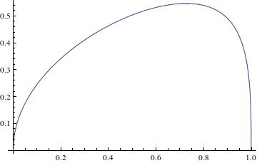
Figure 1: Graph of the function $\Lambda(-k^{2})$.

Finally, following the standard calculation [66, 67], we compute the observable that would correspond to the energy of a $q\bar{q}$-pair (defined in relativistic gauge theories by introducing external quarks into the theory, and measuring their potential), by subtracting from the string action the action of two ‘rods’ that would fall from the end of the space to the boundary. The renormalized energy is obtained to be

$$V_{q\bar{q}}(r_{max}) =2\int_{0}^{r_{max}}dr\frac{g^{2}(r)}{\sqrt{g^{2}(r)-g^{2}(r_{max})}}-2\int_{0}^{r_{max}}dr\;g(r)$$

$$=\frac{\sqrt{2v_{\xi}}L^{2}}{r_{max}}\int_{0}^{1}dw\left[\frac{(2w^{-2}-fv_{\xi}r^{2}_{max})}{\sqrt{\left(1-\frac{(fv_{\xi}r^{2}_{max}-2)}{2}w^{2}\right)\left(1-w^{2}\right)}}\right.$$ (4.55)

$$\left.-2\frac{1}{w^{2}}\sqrt{\left(1-\frac{fv_{\xi}r^{2}_{max}}{2}w^{2}\right)}\right]\;$$

$$=\frac{\sqrt{2v_{\xi}}L^{2}}{r_{max}}\left({\cal I}_{-2}(k,w^{-2})+{\cal I}_{0}(k,w^{0})-{\cal I}_{g}(k^{\prime},w^{-2})\right)\;,$$ (4.56)

where $k^{\prime}=fv_{\xi}r^{2}_{max}/2$.

We can easily see that

$${\cal I}_{0}(k,w^{0})=\int_{0}^{1}dw\frac{-fv_{\xi}r^{2}_{max}}{\sqrt{\left(1-\frac{(fv_{\xi}r^{2}_{max}-2)}{2}w^{2}\right)\left(1-w^{2}\right)}}=-fv_{\xi}r^{2}_{max}\mathbf{K}(k)\;.$$ (4.57a)

Consider the substitution $$w=\sin u$$, so that the second integral is

$$\begin{split}{\cal I}_{-2}(k,w^{-2})&=2\int_{0}^{\pi/2}du\frac{1}{\sin^{2}u\sqrt{\left(1-\frac{(fv_{\xi}r^{2}_{max}-2)}{2}\sin^{2}u\right)}}\\ &=2\left[\mathbf{K}(k)-\mathbf{E}(k)\right]-2\left.\sqrt{\left(1-\frac{(fv_{\xi}r^{2}_{max}-2)}{2}\sin^{2}u\right)}\cot u\right|_{0}^{\pi/2}\;,\end{split}$$ (4.57b)

and the third integral reads (considering the $$arcsin 2\pi n$$ modulo )

$$\begin{split}{\cal I}_{g}(k,w^{-2})&=2\int_{0}^{\pi/2}du\frac{\cos u}{\sin^{2}u}\sqrt{\left(1-\frac{fv_{\xi}r^{2}_{max}}{2}\sin^{2}u\right)}\\ &=-\left[2\sqrt{\left(1-\frac{fv_{\xi}r^{2}_{max}}{2}\sin^{2}u\right)}\csc u\right.\cr&\left.\left.-\sqrt{2fv_{\xi}r^{2}_{max}}\arcsin\left(\sqrt{\frac{fv_{\xi}r^{2}_{max}}{2}}\sin u\right)\right]\right|_{0}^{\pi/2}\cr&+2\pi n\sqrt{2fv_{\xi}r^{2}_{max}}\;.\end{split}$$ (4.57c)

The terms with $\arcsin(\,\cdots)$ and the terms in the upper limit $u\to\frac{\pi}{2}$ are constants, but we observe that we have two divergent terms for $u\to 0$, namely

$$\begin{split}I=&-2\sqrt{\left(1-\frac{fv_{\xi}r^{2}_{max}}{2}\sin^{2}u\right)}\csc u\\ II=&-2\sqrt{\left(1-\frac{(fv_{\xi}r^{2}_{max}-2)}{2}\sin^{2}u\right)}\cot u\;,\end{split}$$ (4.58)

and the difference in the equation (4.56) gives

$$\lim_{u\to 0}\left(-\sqrt{\left(1-\frac{fv_{\xi}r^{2}_{max}}{2}\sin^{2}u\right)}\csc u+\sqrt{\left(1-\frac{(fv_{\xi}r^{2}_{max}-2)}{2}\sin^{2}u\right)}\cot u\right)=0\;.$$ (4.59)

All in all, if $n\in\mathbb{Z}$, the potential energy $V_{q\bar{q}}$ is

$$\begin{split}V_{q\bar{q}}(r_{max})&=\frac{\sqrt{2v_{\xi}}L^{2}}{r_{max}}\left[(2-fv_{\xi}r^{2}_{max})\mathbf{K}(k)-2\mathbf{E}(k)-2\pi n\sqrt{2fv_{\xi}r^{2}_{max}}\phantom{\frac{1}{2}}\right.\\ &\hskip 56.9055pt\left.+\sqrt{2fv_{\xi}r_{max}^{2}}\arcsin\left(\sqrt{\frac{fv_{\xi}r_{max}^{2}}{2}}\right)+2\sqrt{1-\frac{fv_{\xi}r_{max}^{2}}{2}}\right]\;.\end{split}$$ (4.60a)

Since $$v_{\xi}\in\left(0,\frac{2}{fr_{max}^{2}}\right) v_{\xi}=\frac{a}{fr_{max}^{2}} a\in(0,2)$$, we write with , such that

$$\begin{split}\widehat{V}_{q\bar{q}}(r_{max})=\frac{1}{L^{2}v_{\xi}\sqrt{f}}V_{q\bar{q}}(r_{max})&=\frac{1}{\sqrt{k^{2}+1}}\left[-2\left(k^{2}\mathbf{K}(k)+\mathbf{E}(k)\right)-2\pi n\sqrt{2a}\phantom{\frac{1}{2}}\right.\\ &\hskip 56.9055pt\left.+\sqrt{2a}\arcsin\left(\sqrt{\frac{a}{2}}\right)+2\sqrt{1-\frac{a}{2}}\;\right]\;.\end{split}$$ (4.60b)

In the figure 2, we plot the graph for three different values of $$a$$.

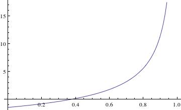
(a) $a=0.1$

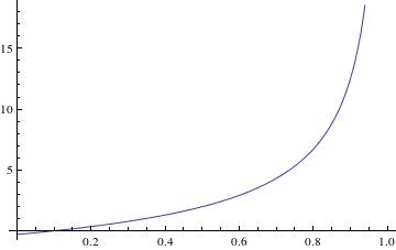
(b) $a=1.0$

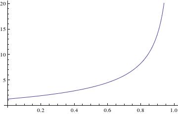
(c) $a=1.9$

Figure 2: Graph of $\widehat{V}_{q\bar{q}}$ against $-k^{2}$, for three different values of $a$ and $n=0$.

Alternatively, we can write the energy as a function of the distance, $\ell_{q\bar{q}}$, as

$$\begin{split}V_{q\bar{q}}(r_{max})=\frac{L^{2}\sqrt{2v_{\xi}}}{r_{max}}&\left[-2\left(\frac{k^{2}\sqrt{fv_{\xi}}}{2\sqrt{2}}\sqrt{\frac{-k^{2}}{1+k^{2}}}\ell_{q\bar{q}}+\frac{a}{2}\mathbf{E}(k)\right)\right.-2\pi n\sqrt{2a}\\ &\left.+\sqrt{2a}\arcsin\left(\sqrt{\frac{a}{2}}\right)+2\sqrt{1-\frac{a}{2}}\;\right].\end{split}$$ (4.60c)

and from this last result we see that

$$\frac{dV_{q\bar{q}}}{d\ell_{q\bar{q}}}=L^{2}\frac{(\sqrt{f}v_{\xi})k^{4}/\sqrt{-k^{2}}}{r_{max}(1+k^{2})^{1/2}}>0\;,\quad\frac{d^{2}V_{q\bar{q}}}{d\ell_{q\bar{q}}^{2}}=0\;.$$ (4.61)

It is important to notice that, although the potential energy $V_{q\bar{q}}$ exhibits a linear behaviour in relation to the distance $\ell_{q\bar{q}}$, similar to confining theories, we can not say that this theory is confining, since we have a maximum value for the distance $\ell_{q\bar{q}}$ in relation to the maximum distance $r_{max}$. Therefore, if we suppose that $\ell_{q\bar{q}}<\ell_{max}$, the potential $V_{q\bar{q}}$ is a bounded function of $\ell_{q\bar{q}}$. A similar phenomenon also happens in the calculations of Wilson loops at finite temperature [66]. Moreover, as we said, it is not clear if the interpretation imported from the relativistic gauge theories still holds in this case.

5 Discussion

In this article we have studied nonabelian T-duality for non-relativistic holographic duals. In particular, using a NATD transformation we constructed novel examples of non-relativistic spaces with the interpretation of holographic duals, one for a conformal Galilean theory in massless type IIA, one for a conformal Galilean theory in massive type IIA, and two for Lifshitz theories in type IIB, coming from NATD of spaces with $T^{1,1}$ and $Y^{p,q}$ internal spaces.

In order to describe the field theories dual to the non-relativistic gravitational backgrounds, we have calculated the conserved charges of these backgrounds and we compared our results with those obtained in [46].

We have also calculated the Wilson loop observables for the holographic dual spaces, though their true interpretation in the field theory remains to be seen, and it would be very interesting to understand. For the Wilson loops in gravity duals of conformal Galilean theories, we considered that the compact coordinate is constant and we found that the energy potential between quarks is always attractive. For the case of case of gravity dual of spaces with Lifshitz symmetry, we could not consider a constant compact coordinate, and we do not know the field theoretical interpretation for the string moving in this direction. The Wilson loop that we found for this second class of spaces is proportional to the quark-antiquark distance, but the interpretation of this result is not clear.

It would be useful to characterize further the field theories dual to the non-relativistic backgrounds considered in this paper, by studying also other properties, like conductivity or shear viscosity.

Acknowledgements. The research of HN is supported in part by CNPQ grant 301709/2013-0 and FAPESP grants 2013/14152-7 and 2014/18634-9. The work of TA is supported by CNPq grant 140588/2012-4. TA also would like to thank Eoin Ó Colgáin, Özgür Kelekci and Niall Macpherson for useful comments, and Guilherme Martins for help on condensed matter issues.

Appendix A Non-Abelian T-Duality

In this Appendix we review non-Abelian T-duality, which is a transformation on a background that supports an $SU(2)$-structure. In principle we could follow the usual method employed in [38, 40, 47, 58, 59, 78], but here we review the strategy used by [41], which has the advantage of giving a closed form for the fields in the RR sector . Considering a spacetime metric and a Kalb-Ramond two-form given by

$$ds^{2}=G_{\mu\nu}(x)dx^{\mu}dx^{\nu}+2G_{\mu i}(x)dx^{\mu}\tau_{i}+G_{ij}(x)\tau_{i}\tau_{j}$$ (A.1)

$$B=\frac{1}{2}B_{\mu\nu}dx^{\mu}\wedge dx^{\nu}+B_{\mu i}dx^{\mu}\wedge\tau_{i}+\frac{1}{2}B_{ij}\tau_{i}\wedge\tau_{j},$$ (A.2)

in such a way that $\mu,\nu=1,\dots,7$ and all dependence on the $SU(2)$ angles $\theta,\psi,\phi$ is contained in the Maurer-Cartan forms $\tau_{i}$ for $SU(2)$, which satisfy $d\tau_{i}=\frac{1}{2}\epsilon_{ijk}\tau_{j}\wedge\tau_{k}$. Furthermore, in general this background has a non-trivial dilaton $\Phi=\Phi(x)$.

If we define the field $Q$ by its components

$$\begin{split}Q_{\mu\nu}&=G_{\mu\nu}+B_{\mu\nu},\quad Q_{\mu i}=G_{\mu i}+B_{\mu i}\\ Q_{i\mu}&=G_{i\mu}+B_{i\mu},\quad\;E_{ij}=G_{ij}+B_{ij}\;,\end{split}$$ (A.3)

one can show that the nonabelian T-dual background is given by

$$\begin{split}\widehat{Q}_{\mu\nu}&=Q_{\mu\nu}-Q_{\mu i}M_{ij}^{-1}Q_{j\nu},\quad\widehat{E}_{ij}=M_{ij}^{-1}\\ \widehat{Q}_{\mu i}&=Q_{\mu j}M_{ji}^{-1},\qquad\widehat{Q}_{i\mu}=-M_{ij}^{-1}Q_{j\mu},\end{split}$$ (A.4)

where the matrix $M$ is defined by

$$M_{ij}=E_{ij}+\alpha^{\prime}\epsilon_{ijk}v_{k}\;,$$ (A.5)

and $\epsilon_{ijk}$ are the structure constants of the group $SU(2)$ and $v_{i}$ are Lagrange multipliers. Hereafter we absorb the factor of $\alpha^{\prime}$ into $v_{i}$ and we present all the correct factors in the final answers. All in all, the dual fields are written as

$$d\hat{s}^{2} =\widehat{G}_{\mu\nu}(x)dx^{\mu}dx^{\nu}+2\widehat{G}_{\mu i}(x)dx^{\mu}dv^{i}+\widehat{G}_{ij}(x)dv^{i}dv^{j}$$ (A.6a)

$$\widehat{B} =\frac{1}{2}\widehat{B}_{\mu\nu}dx^{\mu}\wedge dx^{\nu}+\widehat{B}_{\mu i}dx^{\mu}\wedge dv^{i}+\frac{1}{2}\widehat{B}_{ij}dv^{i}\wedge dv^{j}\;,$$ (A.6b)

and the one-loop contribution to the dilaton is given by

$$\hat{\phi}=\phi-\frac{1}{2}\ln\left(\frac{\Delta}{\alpha^{\prime 3}}\right)\;,$$ (A.6c)

where $\Delta=\det M$. Besides the spectator fields, the dual theory depends on $\theta,\psi,\phi,v^{i}$, meaning that we have too many degrees of freedom and we need to impose a gauge fixing in order to remove three of these variables.

It is convenient to write the metric as

$$ds_{10}^{2}=ds_{7}^{2}+\sum_{i=1}^{3}e^{2C_{i}}(\tau_{i}+A^{i})^{2}\;,$$ (A.7)

where $A^{i}$ are $SU(2)$-valued gauge fields and $C_{i}$ are scalars. Moreover, we define the vielbeins $\{\mathfrak{e}^{\mu},\mathfrak{e}^{i}\}$, such that

$$\begin{split}\mathfrak{e}^{\mu}&\;\Rightarrow\;ds_{7}^{2}=g_{\mu\nu}dx^{\mu}dx^{\nu}=\sum_{\mu=0}^{6}(\mathfrak{e}^{\mu})^{2}\\ \mathfrak{e}^{i}=e^{C_{i}}(\tau_{i}+A^{i})&\;\Rightarrow\;\sum_{i=1}^{3}e^{2C_{i}}(\tau_{i}+A^{i})^{2}=\sum_{i=1}^{3}(\mathfrak{e}^{i})^{2},\end{split}$$ (A.8)

implying that the components of the metric (A.1) are

$$G_{\mu\nu}=g_{\mu\nu}+\sum_{i=1}^{3}e^{2C_{i}}A^{i}_{\mu}A^{i}_{\nu}\;,\quad G_{\mu i}=e^{2C_{i}}A_{\mu}^{i}\;,\quad G_{ij}=e^{2C_{i}}\delta_{ij}\;.$$ (A.9)

In the same way, it is useful to write the Kalb-Ramond as

$$B=\frac{1}{2}b_{\mu\nu}dx^{\mu}\wedge dx^{\nu}+(\beta_{i}+db_{i})\wedge\tau_{i}+\frac{1}{2}\epsilon_{ijk}b_{k}\tau_{i}\wedge\tau_{j}\;,$$ (A.10)

and the components of (A.2) are

$$B_{\mu\nu}=b_{\mu\nu}\;,\quad B_{\mu i}=\beta_{\mu i}+\partial_{\mu}b_{i}\;,\quad B_{ij}=\epsilon_{ijk}b_{k}\;.$$ (A.11)

We next write the inverse of the matrix $M_{ij}$,

$$M_{ij}^{-1}=\frac{1}{\Delta}\begin{pmatrix}e^{2(C_{2}+C_{3})}+z_{1}^{2}\;&z_{1}z_{2}-e^{2C_{3}}z_{3}\;&z_{1}z_{3}+e^{2C_{2}}z_{2}\\ z_{1}z_{2}+e^{2C_{3}}z_{3}\;&e^{2(C_{1}+C_{3})}+z_{2}^{2}\;&z_{2}z_{3}-e^{2C_{1}}z_{1}\\ z_{1}z_{3}-e^{2C_{2}}z_{2}\;&z_{2}z_{3}+e^{2C_{1}}z_{1}\;&e^{2(C_{1}+C_{2})}+z_{3}^{2}\end{pmatrix}\;,$$ (A.12)

where $\Delta=e^{2(C_{1}+C_{2}+C_{3})}+e^{2C_{1}}z_{1}^{2}+e^{2C_{2}}z_{2}^{2}+e^{2C_{3}}z_{3}^{2}$ and $z_{i}=\alpha^{\prime}v_{i}+b_{i}$. In fact, it is easy to see the general formula for the components of $M^{-1}$ is

$$M_{ij}^{-1}=\frac{1}{\Delta}(z_{i}z_{j}+\delta_{ij}e^{2(C_{1}+C_{2}+C_{3})}e^{-2C_{i}}-\epsilon_{ijk}e^{2C_{k}}z_{k})\;.$$ (A.13)

Using all these equations, the authors of [41] were able to find a closed form for the dual metric and Kalb-Ramond field,

$$\begin{split}d\hat{s}^{2}&=ds^{2}_{7}+\frac{1}{\Delta}\left[(z_{1}Dz_{1}+z_{2}Dz_{2}+z_{3}Dz_{3})^{2}+e^{2(C_{2}+C_{3})}Dz_{1}^{2}\right.\\ &\hskip 62.59596pt\left.+e^{2(C_{1}+C_{3})}Dz_{2}^{2}+e^{2(C_{1}+C_{2})}Dz_{3}^{2}\right]\end{split}$$ (A.14a)

$$\begin{split}&\widehat{B}=\frac{1}{2}B_{\mu\nu}dx^{\mu}\wedge dx^{\nu}-\frac{1}{\Delta}(e^{2C_{1}}z_{1}Dz_{2}\wedge Dz_{3}+e^{2C_{2}}z_{2}Dz_{3}\wedge Dz_{1}+e^{2C_{3}}z_{3}Dz_{1}\wedge Dz_{2})\\ &-Dz_{1}\wedge A_{1}-Dz_{2}\wedge A_{2}-Dz_{3}\wedge A_{3}-z_{1}A_{2}\wedge A_{3}-z_{2}A_{3}\wedge A_{1}-z_{3}A_{1}\wedge A_{2}\;\end{split}$$ (A.14b)

where

$$Dz_{i}=dz_{i}+\beta_{i}-\epsilon_{ijk}z_{j}A^{k}\;.$$ (A.14c)

For the RR sector the authors of [41] have shown explicit closed forms for the dual backgrounds. Considering first a (massive) type IIA sector with fields given by

$$F_{0} =m$$ (A.15a)

$$F_{2} =G_{2}+J_{1}^{i}\wedge(\tau_{i}+A^{i})+\frac{1}{2}\epsilon_{ijk}K_{0}^{i}(\tau_{j}+A^{j})\wedge(\tau_{k}+A^{k})$$ (A.15b)

$$F_{4} =G_{4}+L_{3}^{i}\wedge(\tau_{i}+A^{i})+\frac{1}{2}\epsilon_{ijk}M_{2}^{i}\wedge(\tau_{j}+A^{j})\wedge(\tau_{k}+A^{k})$$

$$+N_{1}\wedge(\tau_{1}+A^{1})\wedge(\tau_{2}+A^{2})\wedge(\tau_{3}+A^{3})\;,$$ (A.15c)

one can find the dual type IIB RR fields as

$$\alpha^{\prime 3/2}\widehat{F}_{1} =mz_{i}e^{C_{i}}\hat{\mathfrak{e}}^{i}-z_{i}J^{i}_{1}-K_{0}^{i}e^{C_{i}}\hat{\mathfrak{e}}^{i}+\epsilon_{ijk}K_{0}^{i}z_{j}e^{-C_{k}}\hat{\mathfrak{e}}^{k}+N_{1}$$ (A.16a)

$$\alpha^{\prime 3/2}\widehat{F}_{3} =me^{C_{1}+C_{2}+C_{3}}\hat{\mathfrak{e}}^{1}\wedge\hat{\mathfrak{e}}^{2}\wedge\hat{\mathfrak{e}}^{3}+e^{C_{1}+C_{2}+C_{3}}\ast_{7}G_{4}+G_{2}\wedge z_{i}e^{C_{i}}\hat{\mathfrak{e}}^{i}$$

$$-\frac{1}{2}\epsilon_{ijk}J_{1}^{i}\wedge e^{C_{j}+C_{k}}\hat{\mathfrak{e}}^{j}\wedge\hat{\mathfrak{e}}^{k}+J_{1}^{i}\wedge e^{-C_{i}}\hat{\mathfrak{e}}^{i}\wedge z_{j}e^{C_{j}}\hat{\mathfrak{e}}^{j}$$

$$+z_{i}K_{0}^{i}e^{2C_{i}}e^{-C_{1}-C_{2}-C_{3}}\hat{\mathfrak{e}}^{1}\wedge\hat{\mathfrak{e}}^{2}\wedge\hat{\mathfrak{e}}^{3}$$ (A.16b)

$$-N_{1}\wedge\frac{1}{2}\epsilon_{ijk}z_{i}e^{-C_{b}-C_{c}}\hat{\mathfrak{e}}^{j}\wedge\hat{\mathfrak{e}}^{k}-z_{i}L_{3}^{i}-M_{2}^{i}\wedge e^{C_{i}}\hat{\mathfrak{e}}^{i}+\epsilon_{ijk}M_{2}^{i}z_{j}\wedge e^{-C_{k}}\hat{\mathfrak{e}}^{k}$$

$$\alpha^{\prime 3/2}\widehat{F}_{5} =(1+\ast)\left[G_{4}\wedge z_{i}e^{C_{i}}\hat{\mathfrak{e}}^{a}i+e^{C_{1}+C_{2}+C_{3}}G_{2}\wedge\hat{\mathfrak{e}}^{1}\wedge\hat{\mathfrak{e}}^{2}\wedge\hat{\mathfrak{e}}^{3}\right.$$ (A.16c)

$$-\frac{1}{2}\epsilon_{ijk}L_{3}^{i}\wedge e^{C_{j}+C_{k}}\hat{\mathfrak{e}}^{j}\wedge\hat{\mathfrak{e}}^{k}$$

$$+\left.L_{3}^{i}\wedge e^{-C_{i}}\hat{\mathfrak{e}}^{i}\wedge z_{j}e^{C_{j}}\hat{\mathfrak{e}}^{j}+z_{i}M_{2}^{i}e^{2C_{i}}\wedge e^{-C_{1}-C_{2}-C_{3}}\hat{\mathfrak{e}}^{1}\wedge\hat{\mathfrak{e}}^{2}\wedge\hat{\mathfrak{e}}^{3}\right]\;.$$ (A.16d)

Reversely, starting from a type IIB solution, with RR-fields given by

$$F_{1} =G_{1}$$ (A.17a)

$$F_{3} =G_{3}+X_{2}^{i}\wedge(\tau_{i}+A^{i})+\frac{1}{2}\epsilon_{ijk}Y_{1}^{i}\wedge(\tau_{j}+A^{j})\wedge(\tau_{k}+A^{k})$$

$$+m(\tau_{1}+A^{1})\wedge(\tau_{2}+A^{2})\wedge(\tau_{3}+A^{3})$$ (A.17b)

$$F_{5} =(1+\ast)\left[Z_{4}^{i}\wedge(\tau_{i}+A^{i})+G_{2}\wedge(\tau_{1}+A^{1})\wedge(\tau_{2}+A^{2})\wedge(\tau_{3}+A^{3})\right]\;,$$ (A.17c)

we have the dual fields in IIA supergravity

$$\widehat{F}_{0} =-m$$ (A.17d)

$$\widehat{F}_{2} =-e^{C_{a}}z_{a}G_{1}\wedge\hat{\mathfrak{e}}^{a}+z_{a}X_{2}^{a}+Y_{1}^{a}\wedge(e^{C_{a}}\hat{\mathfrak{e}}^{a})-\epsilon^{abc}Y_{1}^{a}\wedge(z_{b}e^{-C_{c}}\hat{\mathfrak{e}}^{c})$$

$$+\frac{m}{2}e^{-C_{a}-C_{b}}\epsilon^{abc}z_{c}\hat{\mathfrak{e}}^{a}\wedge\hat{\mathfrak{e}}^{b}-G_{2}$$ (A.17e)

$$\widehat{F}_{4} =e^{C_{1}+C_{2}+C_{3}}\ast_{7}G_{3}-z_{a}Z^{a}_{4}-e^{C_{1}+C_{2}+C_{3}}\ast_{7}Z_{4}^{a}\wedge(e^{-C_{a}}\hat{\mathfrak{e}}^{a})-\epsilon^{abc}e^{-C_{a}}\ast_{7}Z_{4}^{a}\wedge z_{b}e^{C_{b}}\hat{\mathfrak{e}}^{c}$$

$$-e^{C_{a}}z_{a}G_{3}\wedge\hat{\mathfrak{e}}^{a}+\frac{1}{2}G_{2}\wedge(\epsilon^{abc}z_{a}e^{-C_{b}-C_{c}}\hat{\mathfrak{e}}^{b}\wedge\hat{\mathfrak{e}}^{c})+\frac{1}{2}\epsilon^{abc}X_{2}^{a}\wedge(e^{C_{b}+C_{c}}\hat{\mathfrak{e}}^{b}\wedge\hat{\mathfrak{e}}^{c})$$

$$-X_{2}^{a}\wedge(e^{-C_{a}}\hat{\mathfrak{e}}^{a})\wedge(z_{b}e^{C_{b}}\hat{\mathfrak{e}}^{b})-e^{C_{1}+C_{2}+C_{3}}G_{1}\wedge\hat{\mathfrak{e}}^{1}\wedge\hat{\mathfrak{e}}^{2}\wedge\hat{\mathfrak{e}}^{3}$$

$$-z_{a}e^{2C_{a}}Y_{1}^{a}\wedge(e^{-C_{1}-C_{2}-C_{3}}\hat{\mathfrak{e}}^{1}\wedge\hat{\mathfrak{e}}^{2}\wedge\hat{\mathfrak{e}}^{3})$$ (A.17f)

where the dual vielbeins are defined to be

$$\hat{\mathfrak{e}}^{i}=e^{C_{i}}\Delta^{-1}\left\{z_{i}z_{j}Dz_{j}+e^{2\sum_{i\neq j}C_{j}}Dz_{i}+\epsilon_{ijk}z_{j}e^{2C_{j}}Dz_{k}\right\}\;.$$ (A.18)

References

- [1] J. M. Maldacena, “The Large N limit of superconformal field theories and supergravity,” Int.J.Theor.Phys. 38 (1999) 1113–1133, arXiv:hep-th/9711200 [hep-th].
- [2] S. Gubser, I. R. Klebanov, and A. M. Polyakov, “Gauge theory correlators from noncritical string theory,” Phys.Lett. B428 (1998) 105–114, arXiv:hep-th/9802109 [hep-th].
- [3] E. Witten, “Anti-de Sitter space and holography,” Adv.Theor.Math.Phys. 2 (1998) 253–291, arXiv:hep-th/9802150 [hep-th].
- [4] O. Aharony, S. S. Gubser, J. M. Maldacena, H. Ooguri, and Y. Oz, “Large N field theories, string theory and gravity,” Phys.Rept. 323 (2000) 183–386, arXiv:hep-th/9905111 [hep-th].
- [5] P. Anderson, Basic Notions Of Condensed Matter Physics. Advanced Books Classics Series. Westview Press, 2008.
- [6] S. Sachdev, Quantum Phase Transitions. Troisième Cycle de la Physique. Cambridge University Press, 2011.
- [7] Y. Nishida and D. T. Son, “Nonrelativistic conformal field theories,” Phys.Rev. D76 (2007) 086004, arXiv:0706.3746 [hep-th].
- [8] D. Son, “Toward an AdS/cold atoms correspondence: A Geometric realization of the Schrodinger symmetry,” Phys.Rev. D78 (2008) 046003, arXiv:0804.3972 [hep-th].
- [9] K. Balasubramanian and J. McGreevy, “Gravity duals for non-relativistic CFTs,” Phys.Rev.Lett. 101 (2008) 061601, arXiv:0804.4053 [hep-th].
- [10] C. P. Herzog, M. Rangamani, and S. F. Ross, “Heating up Galilean holography,” JHEP 0811 (2008) 080, arXiv:0807.1099 [hep-th].
- [11] J. Maldacena, D. Martelli, and Y. Tachikawa, “Comments on string theory backgrounds with non-relativistic conformal symmetry,” JHEP 0810 (2008) 072, arXiv:0807.1100 [hep-th].
- [12] A. Adams, K. Balasubramanian, and J. McGreevy, “Hot Spacetimes for Cold Atoms,” JHEP 0811 (2008) 059, arXiv:0807.1111 [hep-th].
- [13] S. A. Hartnoll, “Lectures on holographic methods for condensed matter physics,” Class.Quant.Grav. 26 (2009) 224002, arXiv:0903.3246 [hep-th].
- [14] S. Kachru, X. Liu, and M. Mulligan, “Gravity duals of Lifshitz-like fixed points,” Phys.Rev. D78 (2008) 106005, arXiv:0808.1725 [hep-th].
- [15] K. Balasubramanian and K. Narayan, “Lifshitz spacetimes from AdS null and cosmological solutions,” JHEP 1008 (2010) 014, arXiv:1005.3291 [hep-th].
- [16] A. Donos and J. P. Gauntlett, “Lifshitz Solutions of D=10 and D=11 supergravity,” JHEP 1012 (2010) 002, arXiv:1008.2062 [hep-th].
- [17] N. Bobev, A. Kundu, and K. Pilch, “Supersymmetric IIB Solutions with Schrodinger Symmetry,” JHEP 0907 (2009) 107, arXiv:0905.0673 [hep-th].
- [18] A. Donos and J. P. Gauntlett, “Supersymmetric solutions for non-relativistic holography,” JHEP 0903 (2009) 138, arXiv:0901.0818 [hep-th].
- [19] A. Donos and J. P. Gauntlett, “Solutions of type IIB and D=11 supergravity with Schrodinger(z) symmetry,” JHEP 0907 (2009) 042, arXiv:0905.1098 [hep-th].
- [20] H. Ooguri and C.-S. Park, “Supersymmetric non-relativistic geometries in M-theory,” Nucl.Phys. B824 (2010) 136–153, arXiv:0905.1954 [hep-th].
- [21] A. Donos and J. P. Gauntlett, “Schrodinger invariant solutions of type IIB with enhanced supersymmetry,” JHEP 0910 (2009) 073, arXiv:0907.1761 [hep-th].
- [22] H. Singh, “Galilean type IIA backgrounds and a map,” Mod.Phys.Lett. A26 (2011) 1443–1451, arXiv:1007.0866 [hep-th].
- [23] J. Jeong, H.-C. Kim, S. Lee, E. Ó Colgáin, and H. Yavartanoo, “Schrödinger invariant solutions of M-theory with Enhanced Supersymmetry,” JHEP 1003 (2010) 034, arXiv:0911.5281 [hep-th].
- [24] R. Gregory, S. L. Parameswaran, G. Tasinato, and I. Zavala, “Lifshitz solutions in supergravity and string theory,” JHEP 12 (2010) 047, arXiv:1009.3445 [hep-th].
- [25] S. M. Ko, C. Melby-Thompson, R. Meyer, and J.-H. Park, “Dynamics of Perturbations in Double Field Theory and Non-Relativistic String Theory,” arXiv:1508.01121 [hep-th].
- [26] J. P. Gauntlett, D. Martelli, J. Sparks, and D. Waldram, “Supersymmetric AdS backgrounds in string and M-theory,” arXiv:hep-th/0411194 [hep-th].
- [27] U. Gran, G. Papadopoulos, and D. Roest, “Systematics of M-theory spinorial geometry,” Class.Quant.Grav. 22 (2005) 2701–2744, arXiv:hep-th/0503046 [hep-th].
- [28] C. I. Lazaroiu and E.-M. Babalic, “Geometric algebra and M-theory compactifications,” Rom.J.Phys. 58 (2013) 5–6, arXiv:1301.5094 [hep-th].
- [29] T. Buscher, “Path Integral Derivation of Quantum Duality in Nonlinear Sigma Models,” Phys.Lett. B201 (1988) 466.
- [30] M. Rocek and E. P. Verlinde, “Duality, quotients, and currents,” Nucl.Phys. B373 (1992) 630–646, arXiv:hep-th/9110053 [hep-th].
- [31] A. Giveon and M. Rocek, “Generalized duality in curved string backgrounds,” Nucl.Phys. B380 (1992) 128–146, arXiv:hep-th/9112070 [hep-th].
- [32] E. Álvarez, L. Álvarez-Gaumé, J. Barbon, and Y. Lozano, “Some global aspects of duality in string theory,” Nucl.Phys. B415 (1994) 71–100, arXiv:hep-th/9309039 [hep-th].
- [33] E. Álvarez, L. Álvarez-Gaumé, and Y. Lozano, “An Introduction to T duality in string theory,” Nucl.Phys.Proc.Suppl. 41 (1995) 1–20, arXiv:hep-th/9410237 [hep-th].
- [34] X. C. de la Ossa and F. Quevedo, “Duality symmetries from nonAbelian isometries in string theory,” Nucl.Phys. B403 (1993) 377–394, arXiv:hep-th/9210021 [hep-th].
- [35] A. Giveon and M. Rocek, “On nonAbelian duality,” Nucl.Phys. B421 (1994) 173–190, arXiv:hep-th/9308154 [hep-th].
- [36] M. Gasperini, R. Ricci, and G. Veneziano, “A Problem with nonAbelian duality?,” Phys.Lett. B319 (1993) 438–444, arXiv:hep-th/9308112 [hep-th].
- [37] E. Álvarez, L. Álvarez-Gaumé, and Y. Lozano, “On nonAbelian duality,” Nucl.Phys. B424 (1994) 155–183, arXiv:hep-th/9403155 [hep-th].
- [38] K. Sfetsos and D. C. Thompson, “On non-abelian T-dual geometries with Ramond fluxes,” Nucl.Phys. B846 (2011) 21–42, arXiv:1012.1320 [hep-th].
- [39] Y. Lozano, E. Ó Colgáin, K. Sfetsos, and D. C. Thompson, “Non-abelian T-duality, Ramond Fields and Coset Geometries,” JHEP 1106 (2011) 106, arXiv:1104.5196 [hep-th].
- [40] G. Itsios, C. Núñez, K. Sfetsos, and D. C. Thompson, “Non-Abelian T-duality and the AdS/CFT correspondence: new N=1 backgrounds,” Nucl.Phys. B873 (2013) 1–64, arXiv:1301.6755 [hep-th].
- [41] Ö. Kelekci, Y. Lozano, N. T. Macpherson, and E. Ó Colgáin, “Supersymmetry and non-Abelian T-duality in type II supergravity,” Class.Quant.Grav. 32 (2015) no. 3, 035014, arXiv:1409.7406 [hep-th].
- [42] Y. Lozano, E. Ó Colgáin, D. Rodríguez-Gómez, and K. Sfetsos, “Supersymmetric via T Duality,” Phys.Rev.Lett. 110 (2013) no. 23, 231601, arXiv:1212.1043 [hep-th].
- [43] G. Itsios, C. Núñez, K. Sfetsos, and D. C. Thompson, “On Non-Abelian T-Duality and new N=1 backgrounds,” Phys.Lett. B721 (2013) 342–346, arXiv:1212.4840.
- [44] Y. Lozano, E. Ó Colgáin, and D. Rodríguez-Gómez, “Hints of 5d Fixed Point Theories from Non-Abelian T-duality,” JHEP 1405 (2014) 009, arXiv:1311.4842 [hep-th].
- [45] E. Caceres, N. T. Macpherson, and C. Núñez, “New Type IIB Backgrounds and Aspects of Their Field Theory Duals,” JHEP 1408 (2014) 107, arXiv:1402.3294 [hep-th].
- [46] Y. Lozano and N. T. Macpherson, “A new AdS4/CFT3 dual with extended SUSY and a spectral flow,” JHEP 1411 (2014) 115, arXiv:1408.0912 [hep-th].
- [47] T. R. Araujo and H. Nastase, “ SUSY backgrounds with an AdS factor from non-Abelian T duality,” Phys. Rev. D91 (2015) no. 12, 126015, arXiv:1503.00553 [hep-th].
- [48] Y. Bea, J. D. Edelstein, G. Itsios, K. S. Kooner, C. Núñez, et al., “Compactifications of the Klebanov-Witten CFT and new AdS3 backgrounds,” JHEP 1505 (2015) 062, arXiv:1503.07527 [hep-th].
- [49] N. T. Macpherson, “Non-Abelian T-duality, -structure rotation and holographic duals of Chern-Simons theories,” JHEP 11 (2013) 137, arXiv:1310.1609 [hep-th].
- [50] A. Barranco, J. Gaillard, N. T. Macpherson, C. Núñez, and D. C. Thompson, “G-structures and Flavouring non-Abelian T-duality,” JHEP 08 (2013) 018, arXiv:1305.7229 [hep-th].
- [51] J. Gaillard, N. T. Macpherson, C. Núñez, and D. C. Thompson, “Dualising the Baryonic Branch: Dynamic SU(2) and confining backgrounds in IIA,” Nucl. Phys. B884 (2014) 696–740, arXiv:1312.4945 [hep-th].
- [52] K. S. Kooner and S. Zacarías, “Non-Abelian T-Dualizing the Resolved Conifold with Regular and Fractional D3-Branes,” JHEP 08 (2015) 143, arXiv:1411.7433 [hep-th].
- [53] Y. Lozano, N. T. Macpherson, J. Montero, and E. Ó Colgáin, “New T-duals with supersymmetry,” JHEP 08 (2015) 121, arXiv:1507.02659 [hep-th].
- [54] Y. Lozano, N. T. Macpherson, and J. Montero, “A Supersymmetric Solution in M-theory with Purely Magnetic Flux,” arXiv:1507.02660 [hep-th].
- [55] O. Aharony, O. Bergman, D. L. Jafferis, and J. Maldacena, “N=6 superconformal Chern-Simons-matter theories, M2-branes and their gravity duals,” JHEP 0810 (2008) 091, arXiv:0806.1218 [hep-th].
- [56] T. Nishioka and T. Takayanagi, “On Type IIA Penrose Limit and N=6 Chern-Simons Theories,” JHEP 0808 (2008) 001, arXiv:0806.3391 [hep-th].
- [57] M. Cvetic, H. Lu, and C. Pope, “Consistent warped space Kaluza-Klein reductions, half maximal gauged supergravities and CP**n constructions,” Nucl.Phys. B597 (2001) 172–196, arXiv:hep-th/0007109 [hep-th].
- [58] E. Gevorgyan and G. Sarkissian, “Defects, Non-abelian T-duality, and the Fourier-Mukai transform of the Ramond-Ramond fields,” JHEP 1403 (2014) 035, arXiv:1310.1264 [hep-th].
- [59] N. T. Macpherson, C. Núñez, L. A. Pando Zayas, V. G. J. Rodgers, and C. A. Whiting, “Type IIB supergravity solutions with AdS5 from Abelian and non-Abelian T dualities,” JHEP 1502 (2015) 040, arXiv:1410.2650 [hep-th].
- [60] J. P. Gauntlett, D. Martelli, J. Sparks, and D. Waldram, “Sasaki-Einstein metrics on S**2 x S**3,” Adv.Theor.Math.Phys. 8 (2004) 711–734, arXiv:hep-th/0403002 [hep-th].
- [61] C. M. Hull, “Massive string theories from M theory and F theory,” JHEP 11 (1998) 027, arXiv:hep-th/9811021 [hep-th].
- [62] A. Smilga, Lectures on Quantum Chromodynamics. World Scientific, 2001.
- [63] H. Nastase, Introduction to the AdS/CFT Correspondence. Cambridge University Press, 2015.
- [64] J. Erdmenger and M. Ammon, Gauge/gravity duality. Foundations and applications. Cambridge University Press, 2015.
- [65] H. Nastase, “Introduction to AdS-CFT,” arXiv:0712.0689 [hep-th].
- [66] J. Sonnenschein, “What does the string / gauge correspondence teach us about Wilson loops?,” arXiv:hep-th/0003032 [hep-th].
- [67] C. Núñez, M. Piai, and A. Rago, “Wilson Loops in string duals of Walking and Flavored Systems,” Phys.Rev. D81 (2010) 086001, arXiv:0909.0748 [hep-th].
- [68] T. R. Araujo and H. Nastase, “Comments on the T-dual of the gravity dual of D5-branes on S3,” JHEP 1504 (2015) 081, arXiv:1409.7333 [hep-th].
- [69] U. H. Danielsson and L. Thorlacius, “Black holes in asymptotically Lifshitz spacetime,” JHEP 0903 (2009) 070, arXiv:0812.5088 [hep-th].
- [70] J. Kluson, “Open String in Non-Relativistic Background,” Phys.Rev. D81 (2010) 106006, arXiv:0912.4587 [hep-th].
- [71] K. B. Fadafan, “Drag force in asymptotically Lifshitz spacetimes,” arXiv:0912.4873 [hep-th].
- [72] H. M. Siahaan, “On non-relativistic potential via Wilson loop in Galilean space-time,” Mod.Phys.Lett. A26 (2011) 1719–1724, arXiv:1106.5008 [hep-th].
- [73] K. B. Fadafan and F. Saiedi, “On Holographic Non-relativistic Schwinger Effect,” arXiv:1504.02432 [hep-th].
- [74] C. Bachas, “Convexity of the Quarkonium Potential,” Phys.Rev. D33 (1986) 2723.
- [75] R. E. Arias and G. A. Silva, “Wilson loops stability in the gauge/string correspondence,” JHEP 1001 (2010) 023, arXiv:0911.0662 [hep-th].
- [76] A. Jeffrey and D. Zwillinger, Table of Integrals, Series, and Products. Elsevier Science, 2000.
- [77] P. Byrd and M. Friedman, Handbook of Elliptic Integrals for Engineers and Physicists. Grundlehren der mathematischen Wissenschaften. Springer Berlin Heidelberg, 2013.
- [78] K. Sfetsos and D. C. Thompson, “New supersymmetric backgrounds in Type IIA supergravity,” JHEP 1411 (2014) 006, arXiv:1408.6545 [hep-th].