The dynamics of an articulated $n$-trailer vehicle

Abstract.

We derive the reduced equations of motion for an articulated $n$-trailer vehicle that moves under its own inertia on the plane. We show that the energy level surfaces in the reduced space are $(n+1)$-tori and we classify the equilibria within them, determining their stability. A thorough description of the dynamics is given in the case $n=1$.

1. Introduction

We consider the dynamics of an articulated $n$-trailer vehicle that moves under its own inertia. Such system consists of a leading car, or truck, that is pulling $n$ trailers, like a luggage carrier in the airport. The leading car and the trailers form a convoy that is subjected to $(n+1)$-nonholonomic constraints, one for each body.

This system is a canonical example in nonholonomic motion planning, which is fundamental in robotics, and has been extensively considered from the control perspective (see e.g. [12, 14, 13] and the references therein).

The constraint distribution defined by the $n$-trailer system has also received interest in differential geometry. It is a Goursat distribution (see [9]) and, as shown in [15], all possible Goursat germs of corank $n+1$ are realized at its different points.

The dynamics of wheeled vehicles moving on the plane has been considered in e.g. [1, 7, 3]. The first two of these deal with certain properties of the $n$-trailer system. However, the majority of the existing references to this system deal with its kinematics and disregard its dynamical aspects. To the best of our knowledge, a detailed study of the dynamics of the $n$-trailer system is missing.

The nonholonomic constraints in the $n$-trailer system arise by assuming that each of the bodies in the convoy has a pair of wheels that prohibit motion in the direction perpendicular to them. Each of these constraints is identical to the nonholonomic constraint for the well-known Chaplygin sleigh problem [5]. Hence, the articulated $n$-trailer vehicle is a generalization of the Chaplygin sleigh system that is recovered when the number of trailers $n=0$. (Other generalizations of the Chaplygin sleigh are considered in [2]).

We mention the thorough understanding of the dynamics of the Chaplygin sleigh has resulted in the design of control algorithms, where the control mechanism moves the center of mass [17]. We are hopeful that the results in this paper will turn out to be useful for control purposes.

The outline of the paper is as follows. In Section 2 we introduce the system and the notation that we will follow in our work. We define the configuration space, the nonholonomic constraints and we write down the kinetic energy of the system. We also discuss the related $SE(2)$ symmetry of the problem and describe the reduced space. In Section 3 we derive the reduced equations of motion (3.1). Our approach follows the method suggested in [8]. We show that the energy level sets are diffeomorphic to $(n+1)$-tori, and we give working expressions for the restriction of the flow to them. Section 4 considers the equilibria of the system assuming that the center of mass of the leading car is displaced a distance $a>0$ from the wheel’s axis. We give a complete classification of all the equilibria in an energy level set and perform their linear stability analysis. It is found that the straight line motion of the convoy in the direction of the center of mass of the leading car and with all of the trailers aligned behind it, is asymptotically stable. In Section 5 we deal with the case where the center of mass of the car lies on its wheels’ axis. We give necessary and sufficient conditions on the velocities for the existence of equilibria of the reduced system and we do an exhaustive treatment of the case $n=1$. Finally, in Section 6 we comment on the interest to analyze the influence of the singular configurations on the dynamics.

2. The $n$-trailer mobile vehicle

Following [12, 14] and other references given in these works, we consider a multi-body car system $(\mathcal{B}_{0},\mathcal{B}_{1},\dots,\mathcal{B}_{n})$ that consists of a car $\mathcal{B}_{0}$ pulling $n$ trailers, $\mathcal{B}_{1},\dots,\mathcal{B}_{n}$. The trailers form a convoy (like in a luggage carrier) that moves on the plane (see Figure 2.1 for the case $n=2$).

Each body in the convoy has a set of wheels and we denote by $(x_{i},y_{i})$ the coordinates of the midpoint of the wheel’s axis ($i=0,\dots,n$) with respect to a chosen cartesian frame. The orientation of $\mathcal{B}_{i}$ is determined by the angle $\theta_{i}$ between the main axis of the body and the $x$ axis of the chosen frame (see Figure 2.1).

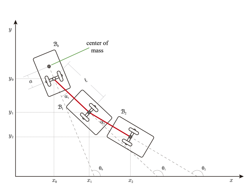
Figure 2.1. The $n$-trailer vehicle with $n=2$.

2.1. Kinematics.

The convoy condition requires that the body $\mathcal{B}_{i}$ is hooked to the preceding body $\mathcal{B}_{i-1}$. Following [12, 14] we assume that the hooking is done via a link of length $\ell$ that connects $(x_{i},y_{i})$ with $(x_{i-1},y_{i-1})$ as illustrated in Figure 2.1. The hooking of the convoy thus defines the $2n$ holonomic constraints

$$x_{i}+\ell\cos\theta_{i}-x_{i-1}=0,\qquad y_{i}+\ell\sin\theta_{i}-y_{i-1}=0,\qquad i=1,\dots,n.$$ (2.1)

On the other hand, the wheels on each of the cars impose a nonholonomic constraint that forbids any motion of the given body in the direction perpendicular to its main axis. In this way we get the $n+1$ nonholonomic constraints

$$\dot{x}_{i}\sin\theta_{i}-\dot{y}_{i}\cos\theta_{i}=0,\qquad i=0,1,\dots,n.$$ (2.2)

In view of the holonomic constraints (2.1), the configuration of the convoy is fully determined by the value of the coordinates

$$x_{0},y_{0},\theta_{0},\theta_{1},\dots,\theta_{n}.$$

Therefore, the configuration space of the system is the $n+3$ dimensional manifold $Q=SE(2)\times\mathbb{T}^{n}$ where $SE(2)$ denotes the Euclidean group in the plane and $\mathbb{T}^{n}$ is the $n$-torus. The nonholonomic constraints (2.2) define a rank $2$ constraint distribution $\mathcal{D}$ on $Q$.

2.2. Dynamics.

We assume that the center of mass of the leading car $\mathcal{B}_{0}$ is displaced a distance $a$ from the midpoint of its wheel’s axis $(x_{0},y_{0})$ along the principal axis of the body (see Figure 2.1). Therefore, if $(x_{C},y_{C})$ denote the coordinates of the center of mass of $\mathcal{B}_{0}$, we have

$$x_{C}=x_{0}+a\cos\theta_{0},\qquad y_{C}=y_{0}+a\sin\theta_{0}.$$ (2.3)

We will denote the total mass of $\mathcal{B}_{0}$ by $M$ and its moment of inertia about its center of mass by $J_{0}$. On the other hand, we shall suppose that the trailers $\mathcal{B}_{1},\dots,\mathcal{B}_{n}$ are identical, with their center of mass lying at the midpoint of the wheel’s axis $(x_{i},y_{i})$. Their total mass is denoted by $m$ and the moment of inertia about $(x_{i},y_{i})$ by $J$.

The kinetic energy of the system is given by

$$\mathcal{K}=\frac{1}{2}\left(J_{0}\dot{\theta}_{0}^{2}+M(\dot{x}_{C}^{2}+\dot{y}_{C}^{2})+J\sum_{i=1}^{n}\dot{\theta}_{i}^{2}+m\sum_{i=1}^{n}(\dot{x}_{i}^{2}+y_{i}^{2})\right).$$

Using (2.3) we get

$$\mathcal{K}=\frac{1}{2}\left((J_{0}+Ma^{2})\dot{\theta}_{0}^{2}+M(\dot{x}_{0}^{2}+\dot{y}_{0}^{2})+2Ma\dot{\theta}_{0}(\dot{y}_{0}\cos\theta_{0}-\dot{x}_{0}\sin\theta_{0})+J\sum_{j=1}^{n}\dot{\theta}_{j}^{2}+m\sum_{i=1}^{n}(\dot{x}_{i}^{2}+y_{i}^{2})\right).$$

The Lagrangian of the system $\mathcal{L}:TQ\to\mathbb{R}$ is obtained by expressing the above quantity in terms of the coordinates $(x_{0},y_{0},\theta_{0},\theta_{1},\dots,\theta_{n})$ of $Q$. In order to eliminate $(\dot{x}_{i},\dot{y}_{i})$ we note that the holonomic constraints (2.1) imply

$$x_{i}=x_{0}-\ell\sum_{j=1}^{i}\cos\theta_{j},\qquad y_{i}=y_{0}-\ell\sum_{j=1}^{i}\sin\theta_{j},\qquad i=1,\dots,n.$$ (2.4)

Differentiating the above and adding yields,

$$\begin{split}\sum_{i=1}^{n}(\dot{x}_{i}^{2}+\dot{y}_{i}^{2})&=n(\dot{x}_{0}^{2}+\dot{y}_{0}^{2})+2\ell\sum_{j=1}^{n}(n+1-j)\dot{\theta}_{j}(\dot{y}_{0}\cos\theta_{j}-\dot{x}_{0}\sin\theta_{j})+\ell^{2}\sum_{j=1}^{n}(n+1-j)\dot{\theta}_{j}^{2}\\ &\qquad\qquad+2\ell^{2}\sum_{k=1}^{n-1}\sum_{j=k+1}^{n}(n+1-j)\dot{\theta}_{k}\dot{\theta}_{j}\cos(\theta_{k}-\theta_{j}),\end{split}$$

where we have used the identity

$$\sum_{i=1}^{n}\left[\left(\sum_{j=1}^{i}T_{j}\cos\theta_{j}\right)^{2}+\left(\sum_{j=1}^{i}T_{j}\sin\theta_{j}\right)^{2}\right]=\sum_{j=1}^{n}(n+1-j)T_{j}^{2}+\sum_{k=1}^{n}\sum_{j=k+1}^{n}2(n+1-j)T_{k}T_{j}\cos(\theta_{k}-\theta_{j}),$$

that holds for arbitrary scalars $T_{1},\dots,T_{i}$.

Therefore, the Lagrangian of the system $\mathcal{L}:TQ\to\mathbb{R}$ is given by

$$\begin{split}\mathcal{L}&=\frac{1}{2}\left((J_{0}+Ma^{2})\dot{\theta}^{2}+(M+nm)(\dot{x}^{2}+\dot{y}^{2})+2Ma\dot{\theta}(\dot{y}\cos\theta-\dot{x}\sin\theta)\right.\\ &\left.\qquad+2m\ell\sum_{j=1}^{n}(n+1-j)\dot{\theta}_{j}(\dot{y}\cos\theta_{j}-\dot{x}\sin\theta_{j})+\sum_{j=1}^{n}(J+(n+1-j)m\ell^{2})\dot{\theta}_{j}^{2}\right.\\ &\left.\qquad+2m\ell^{2}\sum_{k=1}^{n}\sum_{j=k+1}^{n}(n+1-j)\dot{\theta}_{k}\dot{\theta}_{j}\cos(\theta_{k}-\theta_{j})\right),\end{split}$$ (2.5)

where we have introduced the simplified notation $x=x_{0},y=y_{0},\theta=\theta_{0}$.

Using again (2.4), we can write the nonholonomic constraints (2.2) in terms of the coordinates $(x,y,\theta,\theta_{1},\dots,\theta_{n})$ of $Q$ as

$$\dot{x}\sin\theta_{i}-\dot{y}\cos\theta_{i}+\ell\sum_{j=1}^{i}\cos(\theta_{i}-\theta_{j})\dot{\theta}_{j}=0,\qquad i=0,\dots,n.$$ (2.6)

In principle, using (2.5) and (2.6), one could write down the equations of motion for the system in terms of Lagrange multipliers using the Lagrange-D’Alembert principle (see e.g. [11]). However this approach does not make use of the symmetry of the problem that we discuss next.

2.3. Symmetries.

The system possesses an $SE(2)$ symmetry associated to the arbitrariness of the origin and orientation of the chosen cartesian frame. The action of the matrix

$$g=\left(\begin{array}[]{ccc}\cos\varphi&-\sin\varphi&r\\ \sin\varphi&\cos\varphi&s\\ 0&0&1\end{array}\right)\in SE(2)$$

on the configuration $(x,y,\theta,\theta_{1},\dots,\theta_{n})\in Q$ is given by

$$g\cdot(x,y,\theta,\theta_{1},\dots,\theta_{n})=(x_{0}\cos\varphi-y_{0}\sin\varphi+r,x\sin\varphi+y\cos\varphi+s,\theta+\varphi,\theta_{1}+\varphi,\dots,\theta_{n}+\varphi).$$

It is immediate to check that the Lagrangian (2.5) and the constraints (2.6) are invariant under the tangent lift of this action. It follows that the equations of motion drop to the quotient $\mathcal{D}/SE(2)$ which is a rank two vector bundle over the $n$-torus $\mathbb{T}^{n}$.

We denote the angles between subsequent bodies in the convoy by

$$\alpha_{1}=\theta-\theta_{1},\qquad\alpha_{i}=\theta_{i-1}-\theta_{i},\qquad i=2,\dots,n,$$ (2.7)

see Figure 2.1. The value of these angles is invariant under the $SE(2)$ action defined above and their values serve as coordinates on the base $\mathbb{T}^{n}$ of the reduced space $\mathcal{D}/SE(2)$.

Next, we denote by $u$ the component of the linear velocity of the leading body $\mathcal{B}_{0}$ along its main axis, and by $\omega$ its angular velocity. We have

$$u=\dot{x}\cos\theta+\dot{y}\sin\theta,\qquad\omega=\dot{\theta}.$$

As it shall become clear below, the variables $u,\omega$ serve as linear coordinates on the fibers of the reduced space $\mathcal{D}/SE(2)$. The reduced equations of motion form a set of $n+2$ nonlinear, coupled, first order ordinary differential equations for $u,\omega,\alpha_{1},\dots,\alpha_{n}$.

3. The equations of motion

The purpose of this section is to show the following.

Theorem 3.1.

The reduced equations of motion of the $n$-trailer vehicle are given by

$$\begin{split}\dot{u}&=-\frac{1}{2R(\alpha)}\left(\sum_{k=1}^{n}A_{k}\frac{\partial R}{\partial\alpha_{k}}\right)u^{2}+\frac{Q(\alpha)}{\ell^{2}R(\alpha)}u\omega+\frac{Ma}{R(\alpha)}\omega^{2},\\ \dot{\omega}&=-\frac{Mau\omega}{J_{0}+Ma^{2}},\\ \dot{\alpha}_{1}&=\omega-\frac{u\sin\alpha_{1}}{\ell},\\ \dot{\alpha}_{k}&=\frac{u}{\ell}\left(\prod_{j=1}^{k-2}\cos\alpha_{k}\right)\left(\sin\alpha_{k-1}-\cos\alpha_{k-1}\sin\alpha_{k}\right),\qquad k=2,\dots,n.\end{split}$$ (3.1)

where the coefficients $A_{k}$ are defined by (3.5) below and

$$\begin{split}Q(\alpha)&:=\cos\alpha_{1}\sin\alpha_{1}\left(m\ell^{2}\sum_{j=1}^{n}\left(\prod_{k=2}^{j}\cos^{2}\alpha_{k}\right)-J\prod_{k=2}^{n}\cos^{2}\alpha_{k}\right),\\ R(\alpha)&:=M+m\left(\sum_{j=1}^{n}\prod_{k=1}^{j}\cos^{2}\alpha_{k}\right)+\frac{J}{\ell^{2}}\left(1-\prod_{k=1}^{n}\cos^{2}\alpha_{k}\right),\end{split}$$ (3.2)

where we denote $\alpha=(\alpha_{1},\dots,\alpha_{n})$.

The proof of this theorem follows the approach developed in [8] to obtain the equations of motion of regular mechanical nonholonomic system.

We begin by noting that the relations (2.7) imply

$$\theta_{i}=\theta-\sum_{j=1}^{i}\alpha_{j},\qquad i=1,\dots,n.$$ (3.3)

Using these expressions, we can write the nonholonomic constraints (2.6) as

$$\begin{split}&\dot{x}\sin\theta-\dot{y}\cos\theta=0,\\ &\dot{x}\sin\left(\theta-\sum_{j=1}^{i}\alpha_{j}\right)-\dot{y}\cos\left(\theta-\sum_{j=1}^{i}\alpha_{j}\right)+\ell\sum_{j=1}^{i}\cos\left(\sum_{k=j+1}^{i}\alpha_{k}\right)\left(\dot{\theta}-\sum_{l=1}^{j}\dot{\alpha}_{l}\right)=0,\quad i=1,\dots,n.\end{split}$$

Use $(x,y,\theta,\alpha_{1},\dots,\alpha_{n})$ as coordinates on $Q$ and consider the vector fields on $Q$

$$\begin{split}Z_{1}=\cos\theta\frac{\partial}{\partial x}+\sin\theta\frac{\partial}{\partial y}+\sum_{k=1}^{n}A_{k}\frac{\partial}{\partial\alpha_{k}},\qquad Z_{2}=\frac{\partial}{\partial\theta}+\frac{\partial}{\partial\alpha_{1}},\end{split}$$ (3.4)

where

$$\begin{split}A_{k}&=\frac{1}{\ell}\left(\prod_{j=1}^{k-2}\cos\alpha_{j}\right)\left(\sin\alpha_{k-1}-\cos\alpha_{k-1}\sin\alpha_{k}\right),\qquad k=1,\dots,n.\end{split}$$ (3.5)

In the above expression and in the sequel, we use the convention that the product over an empty range of indices equals $1$ and $\alpha_{0}=0$.

It is readily seen that $Z_{1}$ and $Z_{2}$ are linearly independent. Moreover, using the identities

$$\sin\left(\sum_{j=1}^{i}\alpha_{j}\right)=\sum_{j=1}^{i}\cos\left(\sum_{k=j+1}^{i}\alpha_{k}\right)\left(\prod_{s=1}^{j-1}\cos\alpha_{s}\right)\sin\alpha_{j},$$ (3.7)

$$\sum_{l=1}^{j}\left(\prod_{s=1}^{l-2}\cos\alpha_{s}\right)(\sin\alpha_{l-1}-\cos\alpha_{l-1}\sin\alpha_{l})=-\left(\prod_{s=1}^{j-1}\cos\alpha_{s}\right)\sin\alpha_{j},$$

one can check that $Z_{1}$ belongs to $\mathcal{D}$. It is easy to see that $Z_{2}$ is also a section of $\mathcal{D}$. It follows that $\{Z_{1},Z_{2}\}$ is a basis of sections of $\mathcal{D}$ and any tangent vector $v\in TQ$ belonging to $\mathcal{D}$ can be written as a linear combination

$$v=uZ_{1}+\omega Z_{2},\qquad u,\omega\in\mathbb{R}.$$ (3.8)

The components of the above equation give

$$\begin{split}\dot{x}&=u\cos\theta,\\ \dot{y}&=u\sin\theta,\\ \dot{\theta}&=\omega,\\ \dot{\alpha}_{1}&=\omega-\frac{u\sin\alpha_{1}}{\ell},\\ \dot{\alpha}_{k}&=\frac{u}{\ell}\left(\prod_{j=1}^{k-2}\cos\alpha_{j}\right)\left(\sin\alpha_{k-1}-\cos\alpha_{k-1}\sin\alpha_{k}\right),\qquad k=2,\dots,n.\end{split}$$ (3.9)

Equation (3.8) shows that $u$ and $\omega$ are linear coordinates on the fibers of $\mathcal{D}$. Moreover, the vector fields $Z_{1}$ and $Z_{2}$ are invariant under the $SE(2)$ action defined in Section 2.3 and therefore they constitute a basis of sections of the reduced vector bundle $\mathcal{D}/SE(2)$. It follows that $u$ and $\omega$ can be interpreted as linear coordinates on the fibers of the vector bundle $\mathcal{D}/SE(2)$ as advertised before.

Equations (3.9) are of pure kinematic nature and are well known to the control community (see e.g. [12]). They define the evolution of the variables $\alpha_{1},\dots,\alpha_{n}$ in the reduced space and are consistent with (3.1).

The evolution equation for $\omega$ is of dynamical nature and can be easily obtained by noting that the nonholonomic constraints as written in (2.6) do not impose any restriction on the value of $\dot{\theta}$. Hence, the constraint reaction force written in the coordinates $(x,y,\theta,\theta_{1},\dots,\theta_{n})$ has no component along the $\theta$-direction, and the following dynamical equation holds

$$\frac{d}{dt}\left(\frac{\partial\mathcal{L}}{\partial\dot{\theta}}\right)-\frac{\partial\mathcal{L}}{\partial\dot{\theta}}=0,$$

where $\mathcal{L}$ is given by (2.5). Explicitly we have

$$(J_{0}+Ma^{2})\ddot{\theta}+Ma\frac{d}{dt}(\dot{y}\cos\theta-\dot{x}\sin\theta)=-Ma\dot{\theta}(\dot{x}\cos\theta+\dot{y}\sin\theta).$$

Using (3.9) we obtain

$$\dot{\omega}=-\frac{Mau\omega}{J_{0}+Ma^{2}}$$ (3.10)

as in (3.1).

The evolution equation for $u$ is more difficult to obtain. As mentioned above, we follow the approach taken in [8]. This method to obtain the equations of motion of a nonholonomic system is outlined in the Appendix.

The method requires us to compute the constrained Lagrangian $\mathcal{L}_{c}$ that is the restriction of $\mathcal{L}$ to $\mathcal{D}$. It is the kinetic energy of the system when the nonholonomic constraints are satisfied. In view of the symmetries, its value can be expressed in terms of $u,\omega,\alpha_{1},\dots,\alpha_{n}$. To obtain an explicit expression for $\mathcal{L}_{c}$, start by noticing that (3.3), (3.7) and (3.9) imply

$$\dot{x}=u\cos\theta,\qquad\dot{y}=u\sin\theta,\qquad\dot{\theta}=\omega,\qquad\dot{\theta}_{k}=\frac{u\sin\alpha_{k}}{\ell}\prod_{j=1}^{k-1}\cos\alpha_{j},\quad k=1,\dots,n.$$ (3.11)

Next we prove the following.

Proposition 3.2.

Let $j\geq 1$. If the constraints (3.11) are satisfied, then we have

$$\dot{x}_{j}^{2}+\dot{y}_{j}^{2}=u^{2}\prod_{k=1}^{j}\cos^{2}\alpha_{k}.$$ (3.12)

Proof.

By induction. The case $j=1$ is a simple calculation using (2.4) and (3.11) and is left to the reader. Assume that the result is valid for $j-1\geq 1$. Using (2.1) we write

$$\dot{x}_{j}=\dot{x}_{j-1}+\ell\dot{\theta}_{j}\sin\theta_{j},\qquad\dot{y}_{j}=\dot{y}_{j-1}-\ell\dot{\theta}_{j}\cos\theta_{j}.$$

Hence,

$$\dot{x}_{j}^{2}+\dot{y}_{j}^{2}=\dot{x}_{j-1}^{2}+\dot{y}_{j-1}^{2}+2\ell\dot{\theta}_{j}(\dot{x}_{j-1}\sin\theta_{j}-\dot{y}_{j-1}\cos\theta_{j})+\ell^{2}\dot{\theta}_{j}^{2}.$$ (3.13)

Using (2.4) we write

$$\dot{x}_{j-1}=\dot{x}+\ell\sum_{k=1}^{j-1}\sin\theta_{k}\dot{\theta}_{k},\qquad\dot{y}_{j-1}=\dot{y}-\ell\sum_{k=1}^{j-1}\cos\theta_{k}\dot{\theta}_{k},$$

so that

$$\dot{x}_{j-1}\sin\theta_{j}-\dot{y}_{j-1}\cos\theta_{j}=\dot{x}\sin\theta_{j}-\dot{y}\cos\theta_{j}+\ell\sum_{k=1}^{j-1}\cos(\theta_{j}-\theta_{k})\dot{\theta}_{k}.$$

Now, in view of (3.11) and (3.3) we can write

$$\begin{split}&\dot{x}\sin\theta_{j}-\dot{y}\cos\theta_{j}=-u\sin\left(\sum_{k=1}^{j}\alpha_{k}\right),\\ &\ell\sum_{k=1}^{j-1}\cos(\theta_{j}-\theta_{k})\dot{\theta}_{k}=-\ell\dot{\theta}_{j}+u\sum_{k=1}^{j}\cos\left(\sum_{l=k+1}^{j}\alpha_{l}\right)\sin\alpha_{k}\left(\prod_{s=1}^{k-1}\cos\alpha_{s}\right).\end{split}$$

Using the identity (3.7) we conclude that

$$\dot{x}_{j-1}\sin\theta_{j}-\dot{y}_{j-1}\cos\theta_{j}=-\ell\dot{\theta}_{j}.$$

Therefore, (3.13) becomes

$$\dot{x}_{j}^{2}+\dot{y}_{j}^{2}=\dot{x}_{j-1}^{2}+\dot{y}_{j-1}^{2}-\ell^{2}\dot{\theta}_{j}^{2}.$$

Using the induction hypothesis and (3.11) once more, this becomes

$$\dot{x}_{j}^{2}+\dot{y}_{j}^{2}=u^{2}\prod_{k=1}^{j-1}\cos^{2}\alpha_{k}-u^{2}\sin^{2}\alpha_{j}\prod_{k=1}^{j-1}\cos^{2}\alpha_{k}$$

that is equivalent to (3.12).

∎

It follows immediately from the above proposition, and from (3.11), that, if the nonholonomic constraints are satisfied, the kinetic energy $\mathcal{K}_{j}$ of the $j^{th}$ trailer $\mathcal{B}_{j}$ equals

$$\begin{split}\mathcal{K}_{j}&=\frac{1}{2}\left(J\dot{\theta}_{j}^{2}+m(\dot{x}_{j}^{2}+\dot{y}_{j}^{2})\right)\\ &=\frac{u^{2}}{2}\left(\prod_{k=1}^{j-1}\cos^{2}\alpha_{k}\right)\left(\frac{J}{\ell^{2}}\sin^{2}\alpha_{j}+m\cos^{2}\alpha_{j}\right),\end{split}$$

for $j=1,\dots,n$. For $j=0$ we have

$$\begin{split}\mathcal{K}_{0}&=\frac{1}{2}\left(J_{0}\dot{\theta}^{2}+m(\dot{x}_{C}^{2}+\dot{y}_{C}^{2})\right)\\ &=\frac{1}{2}\left((J_{0}+Ma^{2})\omega^{2}+Mu^{2}\right).\end{split}$$

Therefore, adding up the contributions of all the cars in the convoy, we conclude that the constrained Lagrangian is given by

$$\mathcal{L}_{c}=\frac{1}{2}\left(R(\alpha)u^{2}+(J_{0}+Ma^{2})\omega^{2}\right).$$ (3.14)

Next we prove the following.

Lemma 3.3.

The orthogonal projection of the commutator $[Z_{1},Z_{2}]$ onto $\mathcal{D}$ with respect to the kinetic energy metric defined by the Lagrangian (2.5) is given by

$$\mathcal{C}_{12}^{1}Z_{1}+\mathcal{C}_{12}^{2}Z_{2}$$

where

$$\mathcal{C}_{12}^{1}=\frac{Q(\alpha)}{\ell^{2}R(\alpha)},\qquad\mathcal{C}_{12}^{2}=-\frac{Ma}{J_{0}+Ma^{2}}.$$

Here $Q(\alpha)$ and $R(\alpha)$ are defined by (3.2).

Proof.

We give an indirect proof. In view of the discussion in the Appendix, the evolution equation for $\omega$ can be obtained from the general formula (A.1) with the subindex $b=2$ (for us $v^{1}=u$, $v^{2}=\omega$). Since $\mathcal{L}_{c}$ is independent of $x,y,\theta$ and the vector field $Z_{2}$ is given by (3.4), we obtain

$$\frac{d}{dt}\left(\frac{\partial\mathcal{L}_{c}}{\partial\omega}\right)=\mathcal{C}_{12}^{1}u\frac{\partial\mathcal{L}_{c}}{\partial u}+\mathcal{C}_{12}^{2}u\frac{\partial\mathcal{L}_{c}}{\partial\omega}+\frac{\partial\mathcal{L}_{c}}{\partial\alpha_{1}},$$

where we have used $\mathcal{C}_{12}^{e}=-\mathcal{C}_{21}^{e},\;e=1,2$.

Using the expression (3.14) for $\mathcal{L}_{c}$, the last equation becomes

$$(J_{0}+Ma^{2})\dot{\omega}=\mathcal{C}_{12}^{1}R(\alpha)u^{2}+\mathcal{C}_{12}^{2}(J_{0}+Ma^{2})u\omega+\frac{1}{2}\frac{\partial R}{\partial\alpha_{1}}(\alpha)u^{2}.$$

The above equation should simplify to (3.10) so we conclude that

$$\mathcal{C}_{12}^{1}R(\alpha)+\frac{1}{2}\frac{\partial R}{\partial\alpha_{1}}(\alpha)=0,\qquad\mathcal{C}_{12}^{2}=-\frac{Ma}{J_{0}+Ma^{2}}.$$

The proof is completed by noticing that

$$\frac{\partial R}{\partial\alpha_{1}}(\alpha)=-\frac{2Q(\alpha)}{\ell^{2}}.$$ (3.15)

∎

The equation for $u$ can now be obtained from the general formula (A.1) with the subindex $a=1$. Since $\mathcal{L}_{c}$ is independent of $x,y,\theta$ and the vector field $Z_{1}$ is given by (3.4), we obtain

$$\frac{d}{dt}\left(\frac{\partial\mathcal{L}_{c}}{\partial u}\right)=-\mathcal{C}_{12}^{1}\omega\frac{\partial\mathcal{L}_{c}}{\partial u}-\mathcal{C}_{12}^{2}\omega\frac{\partial\mathcal{L}_{c}}{\partial\omega}+\sum_{k=1}^{n}A_{k}\frac{\partial\mathcal{L}_{c}}{\partial\alpha_{k}},$$

that becomes

$$\frac{d}{dt}(R(\alpha)u)=-\frac{Q(\alpha)}{\ell^{2}}u\omega+Ma\omega^{2}+\frac{1}{2}\sum_{k=1}^{n}A_{k}\frac{\partial R}{\partial\alpha_{k}}u^{2}.$$ (3.16)

On the other hand,

$$\frac{d}{dt}(R(\alpha)u)=u\sum_{k=1}^{n}\frac{\partial R}{\partial\alpha_{k}}\dot{\alpha}_{k}+R(\alpha)\dot{u}.$$ (3.17)

Using that

$$\dot{\alpha}_{1}=\omega+uA_{1},\qquad\dot{\alpha}_{k}=uA_{k},\quad k=2,\dots,n,$$ (3.18)

we can combine (3.16) and (3.17) to give

$$R(\alpha)\dot{u}=-\frac{1}{2}\left(\sum_{k=1}^{n}A_{k}\frac{\partial R}{\partial\alpha_{k}}\right)u^{2}-\frac{\partial R}{\partial\alpha_{1}}u\omega-\frac{Q(\alpha)u\omega}{\ell^{2}}+Ma\omega^{2}.$$ (3.19)

Using (3.15) one shows that equation (3.19) can be written as

$$\dot{u}=-\frac{1}{2R(\alpha)}\left(\sum_{k=1}^{n}A_{k}\frac{\partial R}{\partial\alpha_{k}}\right)u^{2}+\frac{Q(\alpha)}{\ell^{2}R(\alpha)}u\omega+\frac{Ma}{R(\alpha)}\omega^{2},$$ (3.20)

that completes the proof of Theorem 3.1.

3.1. Energy conservation and the flow on the energy level surfaces

We note that, as it is usual with nonholonomic systems, the energy is preserved. In our case, this is the reduced kinetic energy given by the constrained Lagrangian (3.14). If we define

$$\mathcal{E}(\alpha,u,\omega)=\frac{1}{2}\left(R(\alpha)u^{2}+(J_{0}+Ma^{2})\omega^{2}\right),$$ (3.21)

then a direct calculation that uses (3.18) and (3.15) shows that $\mathcal{E}$ is preserved by the flow of equations (3.1).

Let $E>0$. It is natural to parametrize the level set $\mathcal{E}=E$ with the angles $\beta,\alpha_{1},\dots,\alpha_{n}$ where the angle $\beta$ is uniquely determined by the conditions

$$u=\sqrt{\frac{2E}{R(\alpha)}}\cos\beta,\qquad\omega=\sqrt{\frac{2E}{J_{0}+Ma^{2}}}\sin\beta.$$ (3.22)

It follows that the energy level set $\mathcal{E}=E$ is diffeomorphic to the $(n+1)$-torus $\mathbb{T}^{n+1}$. To obtain an evolution equation for $\beta$ we differentiate the above relation for $\omega$ with respect to time to obtain

$$\dot{\omega}=\sqrt{\frac{2E}{J_{0}+Ma^{2}}}\dot{\beta}\cos\beta.$$

Now, combining (3.10) with (3.22) and the above equation we obtain

$$\sqrt{\frac{2E}{J_{0}+Ma^{2}}}\dot{\beta}\cos\beta=-\frac{Ma}{J_{0}+Ma^{2}}\left(\frac{2E}{\sqrt{R(\alpha)(J_{0}+Ma^{2})}}\right)\cos\beta\sin\beta$$

which simplifies to

$$\dot{\beta}=-\frac{Ma}{J_{0}+Ma^{2}}\sqrt{\frac{2E}{R(\alpha)}}\sin\beta,$$ (3.23)

assuming that $\cos\beta\neq 0$. Proceeding in an analogous fashion, differentiating the relation for $u$ in (3.22) with respect to time and using (3.20) we obtain (3.23) provided that $\sin\beta\neq 0$. In conclusion, equation (3.23) holds for any value of $\beta$.

The rest of the equations for the flow restricted to the energy surface are obtained by combining (3.22) with (3.1). We obtain

$$\begin{split}\dot{\alpha}_{1}&=\sqrt{\frac{2E}{J_{0}+Ma^{2}}}\sin\beta-\frac{\sqrt{2E}\sin\alpha_{1}}{\ell\sqrt{R(\alpha)}}\cos\beta,\\ \dot{\alpha}_{k}&=\frac{1}{\ell}\sqrt{\frac{2E}{R(\alpha)}}\left(\prod_{j=1}^{k-2}\cos\alpha_{k}\right)\left(\sin\alpha_{k-1}-\cos\alpha_{k-1}\sin\alpha_{k}\right)\cos\beta,\qquad k=2,\dots,n.\end{split}$$ (3.24)

We summarize the results of this subsection in the following.

Theorem 3.4.

The positive energy level sets of the reduced system (3.1) are diffeomorphic to $(n+1)$-tori that can be parametrized with the angular variables $(\beta,\alpha_{1},\dots,\alpha_{n})$. The restriction of the flow to the torus $\mathcal{E}=E>0$ is described by equations (3.23) and (3.24).

4. Classification and linear stability of equilibria

We study the equilibria of the reduced system restricted to a positive energy level set. Throughout this section we assume that the constant $a>0$.

4.1. Classification of equilibria

Proposition 4.1.

Let $E>0$. There exist exactly $2^{n+1}$ equlibrium points in the energy level set $\mathcal{E}=E$ of the reduced system (3.1). They are given by the conditions

$$u=\pm\sqrt{\frac{2E}{M+nm}},\qquad\omega=0,\qquad\sin\alpha_{k}=0,\quad k=1,\dots,n.$$ (4.1)

Proof.

We make use of the restricted equations (3.23) and (3.24). Imposing $\dot{\beta}=0$ in (3.23) implies

$$\sin\beta=0.$$

Under this condition, from (3.24) we see that we can only have $\dot{\alpha}_{1}=0$ if $\sin\alpha_{1}=0$. Now assume that $\dot{\alpha}_{k}=0$ and $\sin\beta=\sin\alpha_{1}=\dots=\sin\alpha_{k-1}=0$. From (3.24) it follows that $\sin\alpha_{k}=0$. This shows that the only equilibria of the system occur at the points where

$$\sin\beta=\sin\alpha_{1}=\dots=\sin\alpha_{n}=0.$$ (4.2)

Now use (3.2) to show that the value of $R(\alpha)$ at these points is the total mass of the system $M+nm$. The proof is completed by using (3.22). ∎

Assume that we are at an equilibrium configuration with energy $E$. The condition $\omega=0$ implies that the leading car moves along a straight line. It moves at the constant speed $\sqrt{\frac{2E}{M+nm}}$ as indicated by (4.1). The motion is forward (in the direction from the midpoint of the wheel’s axis to the center of mass) if $u>0$ or backwards if $u<0$.

On the other hand, the condition $\sin\alpha_{k}=0$ in (4.1) implies that the $k^{th}$ trailer $\mathcal{B}_{k}$ is aligned with the $(k-1)^{th}$ trailer $\mathcal{B}_{k-1}$. Denote by

$$\sigma_{k}=\cos\alpha_{k}=\pm 1,\qquad k=1,\dots,n.$$ (4.3)

If $\sigma_{k}=1$, then $\mathcal{B}_{k}$ is ‘behind’ $\mathcal{B}_{k-1}$. If $\sigma_{1}=-1$ then $\mathcal{B}_{1}$ ‘overlaps’ with $\mathcal{B}_{0}$ since we assume that the wheels of the leading car are located towards the rear of the vehicle. More generally, if $\sigma_{k+1}=-1$ then $\mathcal{B}_{k+1}$ ‘overlaps’ with $\mathcal{B}_{k-1}$. See Figure 4.1. The situation resembles the equilibria of a chain of $n$ coupled planar pendula.

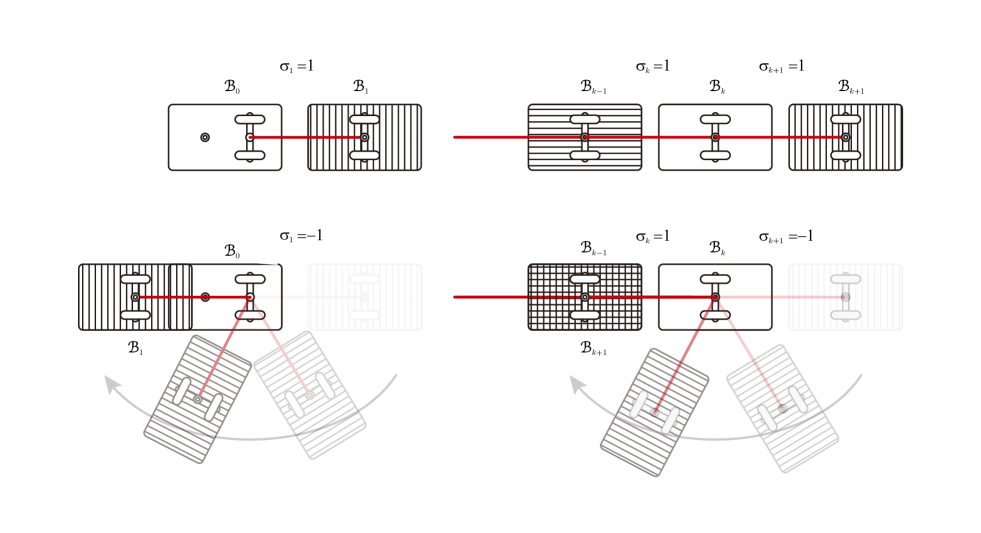
Figure 4.1. Illustration of equilibrium states with $\sigma_{1}=\pm 1$ and with $\sigma_{k}=1$ and $\sigma_{k+1}=\pm 1$.

Therefore, the equilibria of the reduced system correspond to solutions where the convoy moves at constant speed along a straight line with all of the trailers aligned, with the possibility of overlaps between the cars. Of course the only physically attainable equilibria occur when $\sigma_{1}=\cdots=\sigma_{n}=1$ so that there are no overlaps. There are two of such equilibria, corresponding to forward and backward motion of the convoy. We shall see that the former is asymptotically stable whereas the second one is asymptotically unstable.

4.2. Stability of equilibria

We perform a linear stability analysis of the equilibria found in the previous subsection. We will consider the system restricted to the constant energy $(n+1)$-torus $\mathcal{E}=E$, so we work with equations (3.23) and (3.24). To obtain the linearization of these equations around an equilibrium, we shall use the relations

$$R(\alpha)=M+nm,\qquad\frac{\partial R}{\partial\alpha_{j}}(\alpha)=0,\quad j=1,\dots,n,$$

that hold if $\alpha=(\alpha_{1},\dots,\alpha_{n})$ satisfies the equilibrium conditions (4.1).

Fix an equilibrium of equations (3.23) and (3.24) satisfying (4.2). Denote by

$$\sigma_{0}=\cos\beta=\pm 1.$$

Forward motion of the convoy corresponds to $\sigma_{0}=1$ and backward motion to $\sigma_{0}=-1$.

A straightforward calculation shows that the constant $(n+1)\times(n+1)$ matrix that defines the linearization of (3.23) and (3.24) around the given equilibrium is

$$\frac{1}{\ell}\sqrt{\frac{2E}{M+nm}}\left(\begin{array}[]{ccccccc}\frac{-Ma\ell}{J_{0}+Ma^{2}}\sigma_{0}&0&0&0&\cdots&0\\ \ell\sqrt{\frac{M+nm}{J_{0}+Ma^{2}}}\sigma_{0}&-\sigma_{1}\sigma_{0}&0&0&\cdots&0\\ 0&\sigma_{1}\sigma_{0}&-\sigma_{2}\sigma_{1}\sigma_{0}&0&\cdots&0\\ 0&0&\sigma_{2}\sigma_{1}\sigma_{0}&-\sigma_{3}\sigma_{2}\sigma_{1}\sigma_{0}&\cdots&0\\ \vdots&\vdots&&&\ddots&\vdots\\ 0&0&\cdots&\cdots&&-\prod_{j=0}^{n}\sigma_{j}\end{array}\right).$$

Since this matrix is lower diagonal, its eigenvalues are the diagonal components

$$\lambda_{0}=-\frac{Ma}{J_{0}+Ma^{2}}\sqrt{\frac{2E}{M+nm}}\sigma_{0},\qquad\lambda_{k}=-\frac{1}{\ell}\sqrt{\frac{2E}{M+nm}}\prod_{j=0}^{k}\sigma_{j},\quad k=1,\dots,n.$$

Therefore all of the equilibria are hyperbolic. Moreover, we immediately conclude the following about the nature of the equilibria.

1. If at least one of $\sigma_{k}$ with $k=1,\dots,n$, is negative (there are overlaps between the trailers) then there are positive and negative eigenvalues and the equilibrium is a saddle point.

2. If $\sigma_{k}=1$ for all $k=1,\dots,n$ (there are no overlaps) and $\sigma_{0}>0$ (the convoy is moving forwards) then all of the eigenvalues are negative and the equilibrium is a stable node.

3. If $\sigma_{k}=1$ for all $k=1,\dots,n$ (there are no overlaps) and $\sigma_{0}<0$ (the convoy is moving backwards) then all of the eigenvalues are positive and the equilibrium is an unstable node.

An illustration of the numerical integration of the dynamics in the case $n=1$ is given in Figure 4.2. Here the constant energy surface is a two-torus. It is seen the the generic initial conditions approach the stable (respectively unstable) node as $t\to\infty$ (respectively as $t\to-\infty$). Figure 4.2 also shows the trajectory of the leading car $\mathcal{B}_{0}$ on the plane for a generic initial condition. It asymptotically approaches steady motion along a straight line. The curve traced by $\mathcal{B}_{0}$ closely resembles the paths followed by the Chaplygin sleigh (see e.g. [16, 2]).

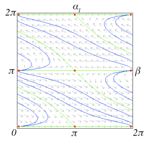
(a) Phase portrait on a fundamental region of the torus $(\alpha_{1},\beta)$. There are 4 equilibrium points (up to equivalence modulo $2\pi$). A stable node at $(0,0)$, an unstable node at $(0,\pi)$ and two saddle points at $(\pi,0)$ and $(\pi,\pi)$.

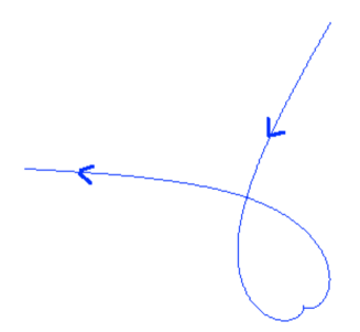
(b) Trajectory of $\mathcal{B}_{0}$ on the plane. Asymptotic behavior towards straight line motion.

Figure 4.2. Phase portrait of the restriction of the reduced flow to an energy level two torus and generic trajectory of the leading car $\mathcal{B}_{0}$ in the case $n=1$.

5. The case $a=0$

If $a=0$ the dynamics changes substantially. From (3.1) we see that $\omega$ is constant throughout the motion.

If $\omega=0$, the classification of the equilibrium solutions of (3.1) coincides with the description given in Proposition 4.1, and the stability of the solution with

$$\sigma_{0}=\sigma_{1}=\cdots=\sigma_{n}=1$$

is analyzed in [7].

For the rest of the paper we consider the case where $\omega\neq 0$. The classification of equilibria is more involved as the following proposition shows.

Proposition 5.1.

Suppose that $a=0$ and that $\omega=\omega_{0}\neq 0$. A necessary and sufficient condition for the existence of equilibria of (3.1) with $u=u_{0}$ is that

$$n\ell^{2}\omega_{0}^{2}\leq u_{0}^{2}.$$ (5.1)

Proof.

Equations (3.18) imply that at such equilibria one must have $u_{0}\neq 0$ and

$$\omega_{0}+u_{0}A_{1}=0,\qquad A_{k}=0,\quad k=2,\dots,n.$$ (5.2)

Using (3.5), the above equations can be written as

$$\begin{split}\sin\alpha_{1}&=\frac{\ell\omega_{0}}{u_{0}},\\ \cos\alpha_{1}\sin\alpha_{2}&=\frac{\ell\omega_{0}}{u_{0}},\\ \vdots\;&\\ \prod_{k=1}^{n-1}\cos\alpha_{k}\sin\alpha_{n}&=\frac{\ell\omega_{0}}{u_{0}}.\end{split}$$

One can inductively show that the solutions to the above equations satisfy

$$\cos^{2}\alpha_{k}=\frac{u_{0}^{2}-k\ell^{2}\omega_{0}^{2}}{u_{0}^{2}-(k-1)\ell^{2}\omega_{0}^{2}},\qquad\sin^{2}\alpha_{k}=\frac{\ell^{2}\omega_{0}^{2}}{u_{0}^{2}-(k-1)\ell^{2}\omega_{0}^{2}},\qquad k=1,\dots,n.$$

It follows that a necessary condition for the existence of equilibria is that

$$\frac{\ell^{2}\omega_{0}^{2}}{u_{0}^{2}-(n-1)\ell^{2}\omega_{0}^{2}}\leq 1,$$

which is equivalent to (5.1). That this condition is also sufficient is seen by noting that if (5.2) holds (and $a=0$), the equation for $\dot{u}$ in (3.1) becomes

$$\dot{u}=\frac{1}{R}\left(\frac{1}{2}\frac{\partial R}{\partial\alpha_{1}}+\frac{Q}{\ell^{2}}\right)u_{0}\omega_{0}.$$

But the right hand side of this equation is zero by (3.15). ∎

The equations for $x,y$ and $\theta$ in (3.9) show that at an equilibrium solution with $u_{0},\omega_{0}\neq 0$ the car $\mathcal{B}_{0}$ moves along a circle of radius $\frac{u_{0}}{\omega_{0}}$ at constant angular speed. Proposition (5.1) shows that the radius of this circle must be at least $\sqrt{n}\ell$.

We do not attempt to study the stability properties of the system in this case. Instead, we treat the case of one trailer in detail.

5.1. The case of one trailer.

If $a=0$ and $n=1$ then, denoting $\alpha_{1}=\alpha$, we have

$$R(\alpha)=M+m\cos^{2}\alpha+\frac{J}{\ell^{2}}\sin^{2}\alpha,$$

and the equations (3.1) become

$$\begin{split}\dot{u}&=\frac{(m\ell^{2}-J)u\cos\alpha\sin\alpha(\ell\omega-u\sin\alpha)}{\ell((M+m\cos^{2}\alpha)\ell^{2}+J\sin^{2}\alpha)}\,,\\ \dot{\omega}&=0,\\ \dot{\alpha}&=\omega-\frac{u\sin\alpha}{\ell}.\end{split}$$ (5.3)

For physical reasons it is natural to assume

$$J<m\ell^{2}.$$ (5.4)

Equations (5.3) are easily integrated using the conservation of energy. First notice that the level sets of the constants $E$ and $\omega$ are invariant circles parametrized by $\alpha$

$$u=\pm\sqrt{\frac{2E-J_{0}\omega^{2}}{R(\alpha)}}.$$

We fix a value of $\omega=\omega_{0}>0$ and we study the behavior of the flow along the invariant circle

$$u=\sqrt{\frac{2E-J_{0}\omega_{0}^{2}}{R(\alpha)}}.$$ (5.5)

The evolution of $\alpha$ along the circle is given by

$$\dot{\alpha}=\frac{\ell\sqrt{R(\alpha)}\omega_{0}-\sqrt{2E-J_{0}\omega_{0}^{2}}\sin\alpha}{\ell\sqrt{R(\alpha)}}$$ (5.6)

which leads to the quadrature

$$\frac{\ell\sqrt{R(\alpha)}\,d\alpha}{\ell\omega_{0}\sqrt{R(\alpha)}-\sqrt{2E-J_{0}\omega_{0}^{2}}\sin\alpha}=dt.$$ (5.7)

Now notice that the inequality (5.4) implies

$$M+\frac{J}{\ell^{2}}\leq R(\alpha)\leq M+m.$$

Using (5.5) and the above inequality, we see that along the solutions of the system we have

$$\begin{split}u^{2}-\ell^{2}\omega_{0}^{2}&=\frac{2E-J_{0}\omega_{0}^{2}}{R(\alpha)}-\ell^{2}\omega_{0}^{2}\\ &\leq\frac{2E-J_{0}\omega_{0}^{2}}{M+\frac{J}{\ell^{2}}}-\ell^{2}\omega_{0}^{2}\\ &=\frac{2(E-E_{c})}{M+\frac{J}{\ell^{2}}}\end{split}$$

where

$$E_{c}:=\frac{1}{2}\left(J_{0}+J+M\ell^{2}\right)\omega_{0}^{2}.$$

The dynamics along the invariant circle (5.5) will depend on how $E$ compares with $E_{c}$.

Case 1. If $\frac{1}{2}J_{0}\omega_{0}^{2}\leq E<E_{c}$.

It follows from Proposition 5.1 (or directly from (5.3)) that there are no equilibrium points of the system in this case. Hence, the dynamics along the invariant circle (5.5) is periodic. The energy dependent period $T=T(E)$ is obtained using (5.7):

$$T=\int_{0}^{2\pi}\frac{\ell\sqrt{R(\alpha)}\,d\alpha}{\ell\omega_{0}\sqrt{R(\alpha)}-\sqrt{2E-J_{0}\omega_{0}^{2}}\sin\alpha}.$$ (5.8)

Using that $E<E_{c}$ one can verify that the denominator does not vanish so this integral is convergent.

Case 2. If $E=E_{c}$.

In this case there is exactly one equilibrium point along the invariant circle (5.5) given by

$$u=\ell\omega_{0},\qquad\alpha=\frac{\pi}{2}.$$

Hence, the invariant circle consists of a homoclinic connection and a critical point.

Case 3. If $E>E_{c}$.

We have

$$0<\frac{\ell^{2}\omega_{0}}{2E-J_{0}\omega_{0}^{2}}<\frac{\ell^{2}\omega_{0}}{2E_{c}-J_{0}\omega_{0}^{2}}=\frac{\ell^{2}}{J+M\ell^{2}}.$$ (5.9)

The graph of the function

$$f(\alpha)=\frac{\sin^{2}\alpha}{R(\alpha)}$$

for $0\leq\alpha\leq\pi$ is shown in Figure 5.1. It is symmetrical with respect to $\alpha=\pi/2$ where it achieves its maximum value of $\frac{\ell^{2}}{J+M\ell^{2}}$. It attains every value between $0$ and $\frac{\ell^{2}}{J+M\ell^{2}}$ exactly two times. It follows from (5.9) that there exist exactly two values of $\alpha$, that we denote by $\alpha^{(1)}$ and $\alpha^{(2)}$, such that

$$0<\alpha^{(1)}<\frac{\pi}{2}<\alpha^{(2)}<\pi\quad\mbox{and}\quad f(\alpha^{(j)})=\frac{\ell^{2}\omega_{0}}{2E-J_{0}\omega_{0}^{2}},\quad j=1,2.$$

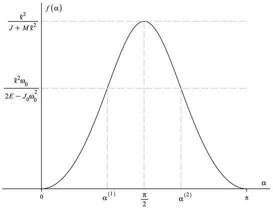
Figure 5.1. Plot of $f(\alpha)$. The horizontal line at height $\frac{\ell^{2}\omega_{0}}{2E-J_{0}\omega_{0}^{2}}$ is drawn under the assumption that $E>E_{c}$.

A short calculation shows that the two points

$$\alpha=\alpha^{(j)},\qquad u=\frac{\omega_{0}\ell}{\sin(\alpha^{(j)})},\qquad j=1,2$$

are the only equilibria of (5.3) contained in the invariant circle (5.5).

Given that $\sin(\alpha^{(j)})>0$, $j=1,2$, in a neighborhood of these points, we can write the evolution equation (5.6) for $\alpha$ as

$$\dot{\alpha}=\omega_{0}-\sqrt{2E-J_{0}\omega_{0}^{2}}\sqrt{f(\alpha)}.$$

Since $f$ is increasing at $\alpha^{(1)}$ and decreasing at $\alpha^{(2)}$ we conclude that the equilibrium

$$\alpha=\alpha^{(j)},\qquad u=\frac{\omega_{0}\ell}{\sin(\alpha^{(j)})}$$ (5.10)

is asymptotically stable if $j=1$ and asymptotically unstable if $j=2$. A physical interpretation of these equilibria can be given with the aid of Figure 5.2.

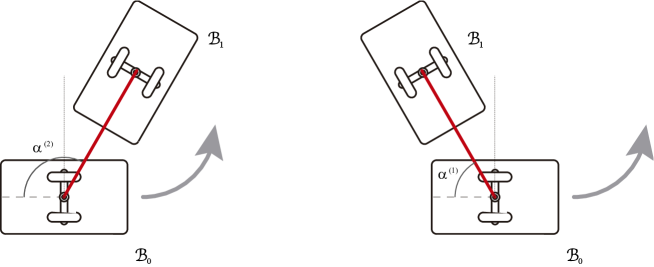
Figure 5.2. Illustration of the unstable and stable equilibria if $E>E_{c}$. The configuration on the left is unstable and on the right is stable. The arrows indicate the motion of $\mathcal{B}_{0}$ (in agreement with our working assumption that $u,\omega_{0}>0$).

Hence, in this case, the invariant circle (5.5) consists of two heteroclinic orbits that connect the unstable critical point with the stable one.

Figure 5.3 illustrates the qualitative dynamics on the invariant circle (5.5) in the three different energy regimes treated above. Figure 5.4 illustrates the dynamics of (5.3) on the cylinder $\omega=\omega_{0}>0$.

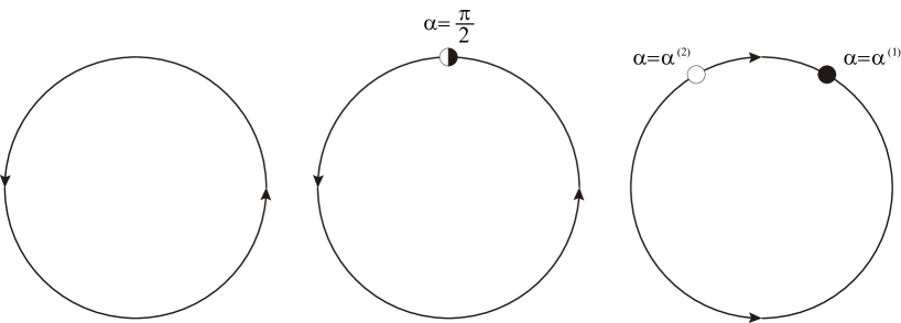
Figure 5.3. Qualitative behavior of the dynamics along the invariant circle (5.5) for the different energy regimes, $E<E_{c}$ on the left, $E=E_{c}$ on the middle and $E>E_{c}$ on the right.

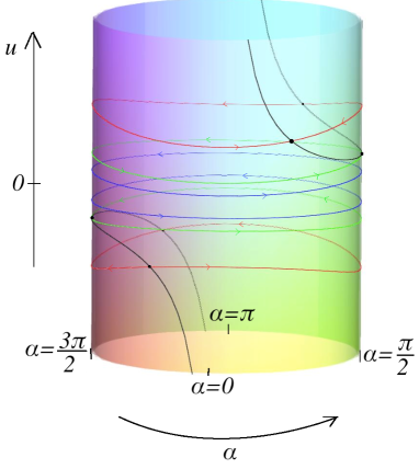
Figure 5.4. Dynamics on the cylinder $\omega=\omega_{0}>0$. The vertical axis is $u$ and the angular variable is $\alpha$. It is seen that the motion takes place along the invariant circles. The critical points are indicated in black. The blue trajectories have $E<E_{c}$, the green ones $E=E_{c}$, and the red ones $E>E_{c}$.

Our analysis shows that $E_{c}$ is a critical value of the energy that separates two different qualitative behaviors. Subcritical energy values lead to periodic motion in the reduced space. On the other hand, supercritical energy values correspond to asymptotic behavior on the reduced space. A similar phenomenon is observed in the motion of a Chaplygin sleigh in a perfect fluid in the presence of circulation [6].

5.1.1. The motion on the plane

With the information given above, we can understand how the $2$-body convoy moves in the plane. First note that in the absence of the trailer $\mathcal{B}_{1}$ (i.e. if $m=0$ and $J=0$) then $u=u_{0},\;\omega=\omega_{0}$ for constants $u_{0}$ and $\omega_{0}$. Hence, the motion of $\mathcal{B}_{0}$ on the plane for a generic initial condition is uniform circular motion on a circle of radius $r=u_{0}/|\omega_{0}|$.

Our analysis in the previous section shows that if $E\geq E_{c}$ in the limit as $t\to\pm\infty$ the $2$-body convoy on the plane approaches uniform circular motion. Continuing with the assumption that $u,\omega_{0}>0$, from (5.10) we conclude that the radii of the limit circles is

$$r=\frac{\ell}{\sin\alpha^{(1)}}=\frac{\ell}{\sin\alpha^{(2)}}.$$

The value of $\sin\alpha^{(1)}=\sin\alpha^{(2)}$ is decreasing and approaches $0$ as the energy $E\to\infty$ so the radius $r\to\infty$ for large energies. Figure 5.5 shows a trajectory of the leading car obtained numerically. The trailer $\mathcal{B}_{1}$ locks itself at a fixed angle with respect to $\mathcal{B}_{0}$ as $t\to\pm\infty$. The limit angles are $\alpha^{(2)}$ when $t\to-\infty$ and $\alpha^{(1)}$ when $t\to\infty$.

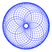
(a) $E<E_{c}$. Generic quasiperiodic trajectory.

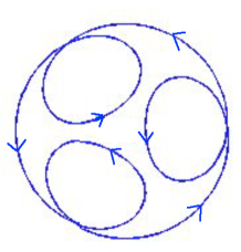
(b) $E<E_{c}$. Periodic trajectory.

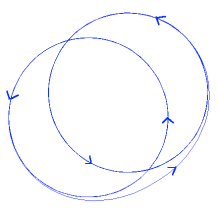
(c) $E>E_{c}$. Asymptotic behavior towards limit circles.

Figure 5.5. Trajectory of the leading car $\mathcal{B}_{0}$ for different energy values.

On the other hand, if $0<E<E_{c}$, the dynamics of $\alpha$ and $u$ is periodic with period (5.8). After one period, the position of the leading car $\mathcal{B}_{0}$ suffers a rotation by an angle $\Delta\theta=\omega_{0}T$, followed by a translation by $(\Delta x,\Delta y)$ with

$$\Delta x+i\Delta y=\int_{0}^{T}u(t)e^{i\omega_{0}t}\,dt=\sqrt{2E-J_{0}\omega_{0}^{2}}\int_{0}^{T}\frac{e^{i\omega_{0}t}}{\sqrt{R(\alpha(t))}}\,dt,$$

where the dependence of $\alpha$ on $t$ is determined by (5.7) and we have assumed that $\theta(0)=0$.

Generically, the angle $\Delta\theta$ is an irrational multiple of $2\pi$ and the motion of $\mathcal{B}_{0}$ in the plane is quasiperiodic with its trajectory contained in an annulus or a circle. It is also possible to have periodic behavior if $\frac{\Delta\theta}{2\pi}\in\mathbb{Q}$ or unbounded trajectories if $\frac{\Delta\theta}{2\pi}\in\mathbb{Z}$ and $\Delta x^{2}+\Delta y^{2}\neq 0$. Figure 5.5 shows a periodic and a quasiperiodic trajectory for $\mathcal{B}_{0}$ obtained numerically.

6. Singular configurations

The degree of nonholonomy is an important notion that arises in nonlinear control theory. It expresses the level of Lie-bracketing of the elements in the constraint distribution that is needed to span the tangent space at each configuration. This concept comes up, for instance, when trying to quantify the complexity associated with steering the system from one point to another (see e.g. [13]).

When the number of trailers in our system is greater than or equal to two, this degree is not constant throughout the configuration space. To fix ideas we treat the case $n=2$ in detail. According to (3.4)

$$\begin{split}Z_{1}=\cos\theta\frac{\partial}{\partial x}+\sin\theta\frac{\partial}{\partial y}-\frac{\sin\alpha_{1}}{\ell}\frac{\partial}{\partial\alpha_{1}}+\left(\frac{\sin\alpha_{1}-\cos\alpha_{1}\sin\alpha_{2}}{\ell}\right)\frac{\partial}{\partial\alpha_{2}},\qquad Z_{2}=\frac{\partial}{\partial\theta}+\frac{\partial}{\partial\alpha_{1}},\end{split}$$

form a basis of the constraint distribution $\mathcal{D}$. Direct calculations show

$$\begin{split}[Z_{1},Z_{2}]=\sin\theta\frac{\partial}{\partial x}-\cos\theta\frac{\partial}{\partial y}+\frac{\cos\alpha_{1}}{\ell}\frac{\partial}{\partial\alpha_{1}}-\left(\frac{\cos\alpha_{1}+\sin\alpha_{1}\sin\alpha_{2}}{\ell}\right)\frac{\partial}{\partial\alpha_{1}},\\ [Z_{1},[Z_{1},Z_{2}]]=\frac{1}{\ell^{2}}\frac{\partial}{\partial\alpha_{1}}-\left(\frac{1+\cos\alpha_{2}}{\ell^{2}}\right)\frac{\partial}{\partial\alpha_{2}},\qquad[Z_{2},[Z_{1},Z_{2}]]=Z_{1},\\ [Z_{1},[Z_{1},[Z_{1},Z_{2}]]]=\frac{\cos\alpha_{1}}{\ell^{3}}\frac{\partial}{\partial\alpha_{1}}-\cos\alpha_{1}\left(\frac{2+\cos\alpha_{2}}{\ell^{3}}\right)\frac{\partial}{\partial\alpha_{2}},\qquad[Z_{2},[Z_{1},[Z_{1},Z_{2}]]]=0.\end{split}$$

Let $q\in Q$ be a configuration of the system with $\cos\alpha_{1}\neq 0$. Then the vector fields $Z_{1},Z_{2},[Z_{1},Z_{2}]$, $[Z_{1},[Z_{1},Z_{2}]]$ and $[Z_{1},[Z_{1},[Z_{1},Z_{2}]]]$ form a basis of the tangent space $T_{q}Q$. The element $[Z_{1},[Z_{1},[Z_{1},Z_{2}]]]$ in the basis is said to have length 4 since one needs to compute iterated brackets of four elements in the basis of $\mathcal{D}$ to generate it. It is clear that it is not possible to construct a basis for $T_{q}Q$ with iterated brackets of $Z_{1}$ and $Z_{2}$ and whose elements have length less than 4. We then say that the degree of nonholonomy at configurations with $\cos\alpha_{1}\neq 0$ is 4.

On the other hand, at configurations $q$ with $\cos\alpha_{1}=0$, the vector field $[Z_{1},[Z_{1},[Z_{1},Z_{2}]]]$ vanishes. One can complete $Z_{1},Z_{2},[Z_{1},Z_{2}]$, $[Z_{1},[Z_{1},Z_{2}]]$ to a basis of $T_{q}Q$ by adjoining the vector field

$$[[Z_{1},Z_{2}],[Z_{1},[Z_{1},Z_{2}]]]=\frac{\sin\alpha_{1}}{\ell^{3}}\frac{\partial}{\partial\alpha_{1}}-\sin\alpha_{1}\left(\frac{2+\cos\alpha_{2}}{\ell^{3}}\right)\frac{\partial}{\partial\alpha_{2}},$$

that has length 5. Hence, the degree of nonholonomy at configurations with $\cos\alpha_{1}\neq 0$ is 5.

The latter configurations are called singular and correspond to having $\mathcal{B}_{0}$ jackknifed, that is, $\mathcal{B}_{0}$ and $\mathcal{B}_{1}$ are perpendicular. It is intuitively clear that maneuvering the system at this configuration is a more difficult task. The classification of singularities for the $n$-trailer vehicle, and the degree of nonholonomy at each of them, is given in [9] for arbitrary $n$. These correspond to different jackknifing possibilities for the bodies in the convoy. A natural question is to understand what are the effects of these singular configurations on the dynamics, if any.

Another example of a nonholonomic system exhibiting singular configurations is an articulated arm. In recent years there have been different efforts to classify the singularities of the associated constraint distribution [18, 4].

To our knowledge, the effect of this kind of singularities on the motion of nonholonomic systems is unexplored. We hope to report on this issue in a future note.

Appendix.

The derivation of the evolution equation for $u$ in (3.1) relies on the method given in [8] to obtain the equations of motion of a mechanical nonholonomic system. This reference includes a more detailed description of the geometry and considers more general cases than what we need. Here we only outline the main steps to obtain (a simple version of) their equations (3.7) and (3.8). Our presentation is done without proof.

Consider a nonholonomic system on a configuration manifold $Q$ of dimension $N$ with Lagrangian $\mathcal{L}:TQ\to\mathbb{R}$ of mechanical type and constraint distribution $\mathcal{D}$ of constant rank $k<N$ that is bracket generating. The condition that $\mathcal{L}$ is of mechanical type means that it is the sum of kinetic minus potential energy, and that the kinetic energy defines a Riemannian metric $\mathcal{G}$ on $Q$.

Associated to the metric $\mathcal{G}$ there is a decomposition $TQ=\mathcal{D}\oplus\mathcal{D}^{\perp}$, where $\mathcal{D}^{\perp}$ is the $\mathcal{G}$-orthogonal complement of $\mathcal{D}$, and a projection $\mathcal{P}:TQ\to\mathcal{D}$.

The idea is to write down the equations of motion that are consistent with the Lagrange d’Alembert principle using quasi-velocities that are adapted to the distribution $\mathcal{D}$. Denote by $q^{1},\dots q^{N}$, local coordinates on an open set of $Q$ and by $Z_{1},\dots,Z_{k}$ a basis of sections of $\mathcal{D}$ in such open set. That is, they are linearly independent vector fields that lie on $\mathcal{D}$.

Define the scalar functions $\rho_{b}^{i}$ and $\mathcal{C}_{bd}^{e}$ on $Q$ through the relations

$$Z_{b}=\rho_{b}^{i}\frac{\partial}{\partial q^{i}},\qquad\mathcal{P}([Z_{b},Z_{d}])=\mathcal{C}_{bd}^{e}Z_{e},\quad b,d,e=1,\dots k,\quad i=1,\dots,N.$$

Let $q\in Q$. Any tangent vector $v\in\mathcal{D}_{q}\subset T_{q}Q$ can be written as

$$v=v^{b}Z_{b}(q)$$

for certain scalars $v^{b}$ (the quasi-velocities). Hence, the value of the restriction of the Lagrangian to $\mathcal{D}$, that we denote as $\mathcal{L}_{c}=\mathcal{L}|_{\mathcal{D}}$, can be expressed in terms of the variables $q^{1},\dots,q^{N},v^{1},\dots,v^{k}$. Equations (3.7) and (3.8) in [8] state that the equations of motion for the nonholonomic system can be written as

$$\dot{q}^{i}=\rho^{i}_{b}v^{b},\qquad i=1,\dots,N,$$

$$\frac{d}{dt}\left(\frac{\partial\mathcal{L}_{c}}{\partial v^{b}}\right)=-\mathcal{C}_{bd}^{e}v^{d}\frac{\partial\mathcal{L}_{c}}{\partial v^{e}}+\rho_{b}^{i}\frac{\partial\mathcal{L}_{c}}{\partial q^{i}},\qquad b=1,\dots,k.$$ (A.1)

These equations avoid dealing with Lagrange multipliers. The effect of the constraint forces is encoded in the effect of the projector $\mathcal{P}$ on the definition of the structure coefficients $\mathcal{C}_{bd}^{e}$.

Acknowledgments

We are thankful to R. Chávez-Tovar for his help to produce some of the figures, and to J.C. Marrero and A.L. Castro for useful conversations and for indicating some references to us. LGN acknowledges the support received from the project PAPIIT IA103815.

References

- [1] Bolzern, P. DeSantis R., Locatelli, A., and Togno, S., Dynamic model of a two-trailer articulated vehicle subject to nonholonomic constraints. Robotica 14 pp 445–450, (1996)
- [2] Borisov A. V. and Mamaev I. S. The dynamics of a Chaplygin sleigh J. of Appl. Math. Mech. 73 pp 156–161, (2009)
- [3] Borisov A.V., Lutsenko S.G. and Mamaev I.S., Dynamics of a wheeled carriage on a plane, Bulletin of Udmurt University. Mathematics, Mechanics, Computer Science, 2010, no. 4, pp. 39–48.
- [4] Castro A. L. and Montgomery R., Spatial curve singularities and the Monster/Semple tower, Israel J. Math. 192, 381–427, (2012).
- [5] Chaplygin, S. A., On the theory of motion of nonholonomic systems. The theorem on the reducing multiplier. Math. Sbornik XXVIII 303–14 (1911) (in Russian)
- [6] Fedorov Y. N., García-Naranjo L. C. and Vankerschaver J., The motion of the 2D hydrodynamic Chaplygin sleigh in the presence of circulation. Disc. and Cont. Dyn. Syst. Series A 33 (2013) no. 9, 4017–4040.
- [7] Fedotov A. B. and Furta S. D., On stability of motion of a chain of driven bodies. Reg. Chaot. Dyn. 7 249–268, (2002).
- [8] Grabowski, J., de León, M., Marrero, J. C. and Martín de Diego, D. Nonholonomic constraints: a new viewpoint. J. Math. Phys. 50 (2009), 013520, 17 pp.
- [9] Jean, F., The car with Trailers: characterization of the singular configurations. ESAIM: Control, Optimisation and Calculus of Variations, 1, 241–266, 1996.
- [10] Lamiraux, F., Sekhavat, S. and Laumond, J.P. Motion Planning and Control for Hilare Pulling a Trailer. Robotics and Automatation, IEEE Transactions on, 15 (1999), 640–652.
- [11] Landau L. D. and Lifshitz E. M. 1976 Mechanics 3rd edn (Oxford:Butterworth-Heinemann).
- [12] Laumond, J.P. Controllability of multibody mobile robot. IEEE Trans. Robot. Automat., 9 (1993), 755–763.
- [13] Laumond J.P. Robot motion planning and control. 1998 Springer, N.ISBN 3-540-76219-1.
- [14] Tilbury D., Murray R., and Sastry S. S., Trajectory generation for the -trailer problem using Goursat normal form, Memo. UCB/ERL M93/12, Berkeley, CA, Feb. 1993.
- [15] Montgomery R. and Zhitomirskii, M., Geometric approach to Goursat flags, Ann. I. H. Poincaré - AN. 18 (2001) 459–493.
- [16] Neimark Ju I and Fufaev N A 1972 Dynamics of Nonholonomic Systems (Translations of Mathematical Monographs vol 33) (Providence, RI: American Mathematical Society)
- [17] Osborne J. and Zenkov, D., Steering the Chaplygin sleigh using a moving mass, Proceeding on the Conference on Decision and Control (CDC-ECC), 2005.
- [18] Pelletier F. and Slayman M., Configurations of an Articulated Arm and Singularities of Special Multi-Flags. SIGMA 10, (2014) 059, 38 pages.