SPF-CellTracker: tracking multiple cells with
strongly-correlated moves using a spatial particle filter

¹Kanazawa University, ²Kyushu Institute of Technology, ³University of Tokyo, ⁴Kyushu University,
⁵Institute of Statistical Mathematics, ⁶JST-CREST. *To whom correspondence should be addressed.

Abstract

Tracking many cells in time-lapse 3D image sequences is an important challenging task of bioimage informatics. Motivated by a study of brain-wide 4D imaging of neural activity in C. elegans, we present a new method of multi-cell tracking. Data types to which the method is applicable are characterized as follows: (i) cells are imaged as globular-like objects, (ii) it is difficult to distinguish cells based only on shape and size, (iii) the number of imaged cells ranges in several hundreds, (iv) moves of nearly-located cells are strongly correlated and (v) cells do not divide. We developed a tracking software suite which we call SPF-CellTracker. Incorporating dependency on cells’ moves into prediction model is the key to reduce the tracking errors: cell-switching and coalescence of tracked positions. We model target cells’ correlated moves as a Markov random field and we also derive a fast computation algorithm, which we call spatial particle filter. With the live-imaging data of nuclei of C. elegans neurons in which approximately 120 nuclei of neurons are imaged, we demonstrate an advantage of the proposed method over the standard particle filter and a method developed by Tokunaga et al. (2014).

1 Introduction

Developments of imaging technologies such as confocal microscopes and fluorescent proteins have increased the demand for computational techniques to process live-cell imaging data, including automatic cell-tracking. Many algorithms for cell-tracking tasks have been developed due to their variety in shape, motion and density [see [21], [16], and [2] for comprehensive surveys]. In the review by Maška et al., they classified these tracking algorithms into two categories, detection and linking and contour evolution based on thier algorithm designs. Methods in the first category tracks cells by two-step procedure: (1) detection of cells in all frames of the video and (2) finding correspondent links of cells in successive frames [1], [3], [13]. In the second category, segmentation and tracking of cells are simultaneously executed by predicting cell positions and evolving the contours of cells in the previous frame to those in the current frame [7], [20]. In addtion to the categories, there is another category called particle filter. Tracking algorithms in this category tracks cells by evolving the probabilistic distribution of cell positions based on the Bayesian recursive formula, instead of estimating cell positions only [22]. All the three categories have their own advantages. A major advantage of methods in the first category is an ability to track new cells entering the field of view since cell positions are determined before tracking. In the second category, robustness for morphological change of living cells is a main advantage. An important advantage of particle filters is that their applicability to arbitrary types of cell shapes since they are typically segmentation-free methods.

Our motivated datasets are 4D live-cell imaging data that capture nuclei of C. elegans. Locations and $\textrm{Ca}^{2+}$ activity levels of neurons can be visualized by incorporating various fluorescent proteins such as mCherry, CFP, and YFP [4]. In order to study the information processing in C. elegans, their neural activities must be measured accurately. For accurate measurements, it is essential to track multiple neurons since neurons of a live nematode move frame by frame according to moves of the nematode itself. In this study, we aim to track more than a hundred of neurons in brain-wide 4D live-cell imaging data of C. elegans. Data types to which the method is applicable are characterized as follows: (i) cells are imaged as globular-like objects, (ii) hundreds of cells are present, (iii) moves of nearly-located cells are strongly correlated with one another, and (iv) cells do not divide. We employ the particle filter as a basis of our tracking algorithm focusing on its scalability to large datasets. We here do not aim at tracking new cells entering the field of view and we focus on tracking cell centroids in order to stabilize tracking performance by avoiding a difficulty in discriminating new cells entering the field of view from cells lost by existing trackers.

Many tracking methods have been developed based on the particle filter in the field of digital image processing. These methods have succeeded in tracking various objects such as human bodies [5, 15], human faces [18, 8], cars [17, 25], and so forth. Applying methods directly to our data often cause problems such as cell-switching: mistaking a cell of interest for one of the other cells. This is mainly due to the following reasons; (1) neuronal nuclei to be imaged are usually ellipsoidal shapes and it is difficult to distinguish them from visual information only, (2) neurons are severely jammed in some areas of the image, and (3) movements of a nematode itself are irregular and sometimes sudden and rapid.

To improve the accuracy of multi-object tracking based on particle filters, Khan et al. proposed a particle filter combined with a Markov random field (MRF) that models dependency on targets’ moves [10]. Smal et al. proposed a method specialized for tracking multiple edges of microtubules during polymerization based on an MRF to avoid collisions of multiple edges [22]. The MRF-based tracking framework is promising but needs to be designed according to characteristics of the dataset. The key feature of our data is that many cells move rapidly but nearly-located cells’ moves are strongly correlated since the change in the cell positions occurs due to the change in body posture of a nematode. Properly modeling such covariation of cells might be the key to reduce the tracking errors.

More recently, we proposed a novel multi-cell tracking method which is based on a MRF model and an optimization technique in order to address the task of tracking hundreds of cells. The proposed method is a novel variant of our previous method [23]: we employ a more sophisticated MRF and the optimization process is replaced by a sampling-based algorithm motivated by the particle filter algorithm. The use of the particle-based tracking combined with the MRF offers two advantages; (i) a great reduction of computational time and (ii) significant improvement of tracking accuracy due to the incorporation of more sophiscated spatial information into the MRF. Through applications to synthetic data and 4D images of neuronal nuclei of C. elegans, we demonstrate that the proposed method indeed outperforms our optimization-based method in terms of tracking performance.

2 Methods

Here we review existing tracking methods with the particle filter. We introduce the particle filter for single object-tracking and its variants for the simultaneous tracking of multiple objects. We then describe our tracking method.

2.1 Existing tracking methods with the particle filter

Particle filter

We begin with a brief introduction of the particle filter (PF), commonly used as a standard object-tracking method. Let $y_{t}$ be the observed image data at time $t$ and let $x_{t}$ denote the state of the target at time $t$. The state includes the target’s information such as location, velocity, volume and shape. The unknown state variables are usually estimated as the filtering distribution $p(x_{t}|y_{1:t})$ where $y_{1:t}=\{y_{1},\cdots,y_{t}\}$. Based on the dynamics of the state $p(x_{t}|x_{t-1})$ and the likelihood $p(y_{t}|x_{t})$, the filtering distribution can be computed based on the following Bayesian recursive formula:

$$p(x_{t}|y_{1:t})\propto p(y_{t}|x_{t})\int p(x_{t}|x_{t-1})p(x_{t-1}|y_{1:t-1})dx_{t-1},$$ (1)

If the dynamics $p(x_{t}|x_{t-1})$ and the likelihood $p(y_{t}|x_{t})$ are linear and Gaussian, these distributions can be exactly calculated by the Kalman filter [9]. These assumptions, however, are too restrictive and unrealistic for object-tracking from video data. Therefore, particle approximation of the distribution is commonly used for dealing with nonlinearity and non-normality of the distribution. The particle filter approximates the filtering distribution by using a set of point masses, i.e., particles. Suppose $N$ is the number of particles, and $\{x_{t}^{(n)}\}_{n=1}^{N}$ is the set of particles which approximates the distribution $p(x_{t}|y_{t-1})$ for one-step-ahead prediction. The particle weight $w_{t}^{(n)}$ is defined as the probability proportional to the likelihood $p(y_{t}|x_{t}^{(n)})$ and can be intuitively interpreted as how much a particle captures the target in the current frame. We also suppose $\{w_{t}^{(n)}\}_{n=1}^{N}$ is the set of particle weights. The filtering distribution is approximated as follows:

$$p(x_{t}|y_{1:t})\approx\sum_{n=1}^{N}w_{t}^{(n)}\delta(x_{t}-x_{t}^{(n)}),$$

where $\delta$ denotes the Dirac delta measure with the mass at $0$. Under this particle approximation, object-tracking is conducted by the following procedure:

1. Prediction: move particles based on the dynamics $p(x_{t}|x_{t-1})$.

2. Filtering: calculate particle weights based on the likelihood $p(y_{t}|x_{t})$.

In Equation (1), the prediction and filtering steps correspond to the calculation of the integral and the multiplication by the likelihood, respectively. We note that particles are usually resampled according to the probabilities proportional to particle weights since the resampling procedure often avoids the degeneracy of the algorithm [6], meaning that the resampling procedure stabilizes the tracking quality. We therefore assume resampling is always conducted in the filtering step and we refer to a set of resampled particles as a filter ensemble, denoted by $\{x_{t|t}^{(n)}\}_{n=1}^{N}$.

Joint particle filter

The standard particle filter has been extended to the tracking of multiple targets. The most basic method is a joint particle filter (JPF), also known as mixture tracking [24]. Suppose $x_{t,k}$ denotes the location of target $k$ at time $t$. We hereafter denote the set of locations for all targets by $x_{t}$. In JPF, the dynamics of the multiple targets is defined as follows:

$$p(x_{t}|x_{t-1})=\prod_{k\in V}p(x_{t,k}|x_{t-1,k}),$$

where $V$ is the index set of all targets. That is, the movements of the targets are assumed to be independent of each other. Therefore, JPF can be computed by an independent run of the standard PF for each target. JPF is a reasonable option of the multi-object tracking if (1) the number of objects to be tracked is moderate, and (2) the visual characteristics of the targets are clearly different. Otherwise, JPF easily fails by tracking an incorrect target located close to the target of interest.

Motion model with Markov random field

Next, we introduce a framework of MRF-incorporated motion models [10]. In many cases, moves of a target are dependent on those of other targets. For example, a fish usually changes its direction when it is going to hit another fish. In this approach, JPF is extended to model such dependecies among targets’ moves based on the MRF, which is plugged into the dynamics of the JPF as follows:

$$p(x_{t}|x_{t-1})\propto\prod_{k\in V}p(x_{t,k}|x_{t-1,k})\prod_{(k_{1},k_{2})\in E}\psi(x_{t,k_{1}},x_{t,k_{2}}),$$

where $E$ is the set of edges in the MRF and $\psi$ is the energy function that represents dependency on moves of targets $k_{1}$ and $k_{2}$. The filtering distribution $p(x_{t}|y_{t})$ can be obtained by moving particles based on the dynamics $p(x_{t,k}|x_{t-1,k})$ and computing particle weights that is defined as the product of the likelihood $p(y_{t}|x_{t,k})$ and the energy function $\psi(x_{t,k},x_{t,k^{\prime}})$ for all $k^{\prime}$ such that $(k,k^{\prime})\in E$. This algorithm is called the joint MRF particle filter. The tracking performance of the joint MRF particle filter, however, strongly depends on the number of particles $N$, since generated particles based on dynamics $p(x_{t}|x_{t-1})$ do not include any information of the energy function and tend to be inaccurate. Instead, the filtering distribution $p(x_{t}|y_{t})$ can also be computed by Markov chain Monte Carlo (MCMC) sampling. One issue of the motion model with MRFs is a trade-off between tracking accuracy and computational efficiency. MCMC sampling stabilizes the tracking performance but its computational cost can be prohibitive due to iterative computation until convergence for each frame. On the contrary, joint MRF-PF is computationally efficient but less accurate. In the next subsection, we propose a novel sampling method that is a better compromise between the joint MRF particle filter and MCMC sampling.

2.2 Spatial particle filter

Figure 1: Outline of the spatial particle filter. (a) An illustrative example of a 4D image dataset for nuclei of C. elegans neurons. (b) Preparation of the algorithm using the initial frame of the dataset: (b1) Detection of cell centroids by the DP-means algorithm. (b2) Construction of a Markov random field that defines correlated moves of cells. Its graph structure is constructed by the minimum spanning tree that spans all the cell centroids in the initial frame. (b3) Determination of the cell corresponding to the root node of the tree. (c) Tracking scheme at time $t$: (c1) Tracking the cell corresponding to the root node by the standard particle filter. (c2-c4) Sequential tracking of remaining cells.

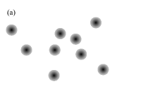
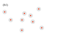
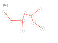
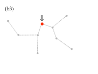
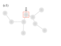
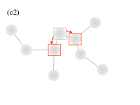
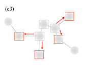
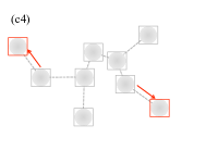
We propose a novel tracking algorithm which we call a spatial particle filter (SPF). Our idea to address the sampling issue of MRF-PF is to design a better proposal distribution that shares information of cells’ dynamics and dependent moves. How do we construct such a better proposal distribution? The sampling inefficiency in the standard particle filter derives from the difficulty in predicting a cell position based only on temporal information since moves of a nematode itself is sometimes sudden and rapid. The key idea to overcome the sampling inefficiency is to incorporate spatial information such as correlated moves among cells into a proposal distribution. If we already know the position of a cell near the target cell in the current and previous frames and the cells’ moves are strongly correlated, the position of the target cell can be efficiently estimated from such correlated moves. We therefore construct a proposal distribution that predicts the target cell position from spatial information, unlikely to motion models in the standard particle filter. The remaining issue is how we determine positions of all cells since all the cell positions are unknown before tracking. A solution is to determine the position of a cell from a nealy-located cell, sequentially. To this end, we transform the joint distribution of state variables for multiple targets at time $t$ into a recursive formula in the spaitial domain, as is similarly done in the temporal domain for the standard PF. Suppose the graph structure of a MRF is restricted to a tree. Let $y_{t,k}$ be the region of the $k$th target image at time $t$, $u(k)$ the parent node of node $k$, $1\rightarrow k$ the path from the root node to node $k$, and $y_{1\rightarrow k}$ the set of regions of target images corresponding to nodes on the path $1\rightarrow k$. Then, the conditional distribution $p(x_{t,k}|y_{1\rightarrow k})$ is represented as the following recursive formula:

$$p(x_{t,k}|y_{t,1\rightarrow k})$$

$$\propto p(y_{t,k}|x_{t,k})\int p(x_{t,k}|x_{t,u(k)})p(x_{t,u(k)}|y_{t,1\rightarrow u(k)})dx_{t,u(k)}.$$

That is, a target can be tracked from the location of a corresponding parent node by the standard PF-like computation for each path for each frame, meaning all targets except for the root node can be tracked by a sweep of the MRF tree as shown in Figure 1(c). In this formula, we design $p(x_{t,k}|x_{t,u(k)})$ as a proposal distribution that shares information of the dynamics of the $k$th target and the energy function between $k$ and $u(k)$. To deal with nonlinearity and non-normality, we approximate the conditional distribution by a set of particles $\{x_{t,k}^{(n)}\}_{n=1}^{N}$ and particle weights $\{w_{t,k}^{(n)}\}_{n=1}^{N}$ as follows:

$$p(x_{t,k}|y_{t,1\rightarrow k})\approx\sum_{n=1}^{N}w_{t,k}^{(n)}\delta(x_{t,k}-x_{t,k}^{(n)}).$$

We note that the recursive formula is valid only when the MRF is restricted to a tree. We therefore automatically construct an MRF tree from the initial locations of the targets, as described later. We also note that the target corresponding to the root node in the MRF tree cannot be tracked by this recursive formula, and so we track the root target by the standard PF.

Detection of initial locations and construction of an MRF tree

We detect initial cell locations of by clustering voxels with local peaks and computing centers of the clusters. In order to reduce computational costs, we collect voxels with strong fluorescent intensities. Here, a strong intensity is defined as a local maximum of fluorescent intensities in a region narrower than the size of a cell nucleus, assuming that local peaks of intensities concentrate on the center of a cell nucleus. To cluster the voxels, we use the DP-means algorithm [12], an extension of the $k$-means algorithm that is not needed to specify the number of clusters $k$. The DP-means algorithm is suitable for our data since (1) it automatically counts the number of clusters i.e. the number of cells, (2) the computation is considerably fast, and (3) the parameter $\lambda$ that controls the cluster radii is determined by prior knowledge of the radii of a cell. To construct a graph structure of a MRF that models correlated moves among cells, we construct a minimum spanning tree that spans all the detected locations of cell nuclei by Kruskal’s algorithm [11]. The outline of the spatial particle filter is summarized in Figure 1.

Particle generation in the spatial domain

We here design a proposal distribution $p(x_{t,k}|x_{t,u(k)})$ that serves as both the dynamics of target $k$ and the energy function between target $k$ and target $u(k)$. Our key ideas for constructing the proposal distribution are (1) simulating the covariation with neighbor cells, (2) maintaining the relative positions of cells in the initial frame, and (3) avoiding collisions with neighbor trackers. Let $\{x_{t,k|k}^{(n)}\}_{n=1}^{N}$ be the ensemble set corresponding to the filtering distribution $p(x_{t,k}|y_{1\rightarrow k})$ and let $\overline{x}_{t,k}$ be the mean vector averaged over the ensemble set. We hereafter abbreviate the parent node $u(k)$ simply to $u$ if the confusion does not occur. One approach to taking the covariation information into account is to generate particle $x_{t,k}^{(n)}$ such that the following approximation holds:

$${x}_{t,k}^{(n)}-\overline{x}_{t-1,k}\approx{x}_{t,u|u}^{(n)}-\overline{x}_{t-1,u},$$

that is, the movement of target $k$ between two successive frames is roughly the same as the movement of its parent node $u$. In fact, this is equivalent to preserving the relative position of $k$ for $u$ in the previous frame, since transposition of the second and third terms yields

$${x}_{t,k}^{(n)}-{x}_{t,u|u}^{(n)}\approx\overline{x}_{t-1,k}-\overline{x}_{t-1,u}.$$

The covariation of cells is utilized by this approach, but relative positions of cells in the initial frame are not conserved, i.e., the distance between a pair of cells can be infinite in the long run. We therefore consider another constraint on particle $x_{t,k}^{(n)}$, such that the relative positions of cells in the initial frame are roughly conserved.

$${x}_{t,k}^{(n)}-{x}_{t,u|u}^{(n)}\approx\overline{x}_{1,k}-\overline{x}_{1,u}.$$

We note relative positions to be conserved do not have to be those in the initial frame and can be arbitrarily chosen from those in all frames if the tracking is offline. Therefore, if we find the frame when the movement of a nematode itself is slower and more stable than that in the initial frame, the frame is a better choice for defining the relative positions of the cells. Let $\eta_{t}^{k_{1},k_{2}}:=\overline{x}_{t,k_{1}}-\overline{x}_{t,k_{2}}$. We construct a proposal distribution $p(x_{t,k}|x_{t,u(k)})$ such that the above two constraints simultaneously hold:

$$x_{t,k}^{(n)}=x_{t,u|u}^{(n)}+\alpha\eta_{t-1}^{k,u}+(1-\alpha)\eta_{1}^{k,u}+v_{t,k}^{(n)},$$ (2)

where $v_{t,k}^{(n)}$ is the noise vector that follows the normal distribution with mean vector $0$ and covariance matrix $\Sigma$, and $\alpha$ is a tuning parameter whose range is $0<\alpha<1$ and controls the importance between the covariation and relative positions. By this construction, relative positions of cells in the initial frame are conserved in the long run since the time series generated from the proposal distribution is stationary. We see this fact by taking the average of Equation (2) over the index set of particles $\{n|1\cdots,N\}$ derives the following autoregressive model:

$$(\eta_{t}^{k,u}-\eta_{1}^{k,u})=\alpha(\eta_{t-1}^{k,u}-\eta_{1}^{k,u})+\overline{v}_{t,k},$$

where $\overline{v}_{t,k}$ is the average of the noise vectors over the index set of particles. Since the autoregressive coefficient $\alpha$ satisfies $0<\alpha<1$, $\eta_{t}^{k,u}$ is a stationary process with mean $\eta_{1}^{k,u}$, meaning that relative positions of cells in the initial frame are conserved in the long run.

The remaining task to construct the procedure of generating particles is to avoid collisions with neighbor trackers. To this end, we combine a rejection sampling with the proposal distribution. After generating a particle based on the proposal distribution, we reject the particle if the distance between $k$ and $u$ is small compared with the radii of a cell nucleus. Formally, we reject the particle with probability proportional to $\exp\{-||\eta_{t}^{k,u}||^{2}/\lambda^{2}\}$, where $\lambda$ denotes the predefined radius of cell nuclei, and accept otherwise.

Calculation of particle weights

We next describe how we evaluate the importance of a particle which tracks a cell nucleus. The point-spread function (PSF) is typically used for evaluating the similarity of objects with ellipsoidal shapes [16]. Cell nuclei in our motivated datasets are roughly ellipsoidal but often slightly deformed. To evaluate similarity between cell nuclei under the existence of the deformation, we define the importance of a particle as a similarity between 3D subimages around the $k$th cell centroid in the initial and current frames. Suppose $y_{t}^{(w)}(x)$ is an augmented vector which corresponds to a 3D subimage at time $t$ with center $x\in\mathbb{R}^{3}$ and window width parameter $w=(w_{1},w_{2},w_{3})\in\mathbb{N}_{0}^{3}$. Here, the window is defined as a set of voxels in the cuboid with center voxel including $x$ and edge lengths $2w_{1}+1$, $2w_{2}+1$, and $2w_{3}+1$. We also suppose that $\hat{x}_{1,k}$ is the initial position of the $k$th cell centroid detected by the DP-means algorithm. We then define a likelihood function of particle $x_{t,k}^{(n)}$ as follows:

$$p(y_{t,k}|x_{t,k}^{(n)})\propto\exp\Bigg{\{}-\frac{||y_{t}^{(w)}(x_{t,k}^{(n)})-y_{1}^{(w)}(\hat{x}_{1,k})||^{2}}{2\sigma^{2}W}\Bigg{\}},$$

where $\sigma^{2}$ is the parameter that controls the variance of the 3D-subimage similarity and $W$ is the number of non-zero elements for the vector defined as the elementwise sum of $y_{t}^{(w)}(x_{t,k}^{(n)})$ and $y_{1}^{(w)}(x_{t,k}^{(n)})$. We note that the difference is averaged over nonzero elements in the elementwise sum of the subimages in order to avoid an unintended similarity increase derived from voxels within the window but outside the nucleus region. We also note that the window parameter $w$ should be chosen to be larger than the maximum size of cell nuclei so that all the information of shapes and intensities are included in the window.

Dealing with the disappearance of targets to be tracked

Another difficulty in tracking cells is that some neurons go out of the image space because of movement of the nematode. We track cells out of the image space by the following scheme. If a generated particle in the prediction step goes out of the image space, we add the particle to a member of the filter ensemble without resampling. The reason why we skip the filtering step for such a particle is that likelihood of the particle cannot be evaluated whereas the particle should be survived considering the possibility that the target truly goes out of the image space.

Software

We developed a software suite SPF-CellTracker. Our software is composed of three executables, convert, track, and view. The first software convert converts a set of 2D images that compose 4D live-cell imaging data into a single file encoded as our original binary format. During conversion, the average subtraction and the 3D median filter can be optionally applied for each 3D image in order to remove background noise and salt-and-pepper noise. The second software track is the main software for detecting and tracking multiple cells based on the SPF algorithm from the converted 4D image file. This software was implemented purely in the C language considering the running speed, which will be presented in the following section. The third software view is to visualize the 4D image data with a tracking result. An interesting feature of this visualization software is an ability to zoom in, zoom out, and rotate 4D image during playing 4D image data. All executables and source codes of convert and track are freely available in the supplementary website (S1) listed in Appendix.

3 Experiments

We here present comparisons of cell-tracking and cell-detection performance using synthetic data and real 4D live-cell imaging data. All of supplementary videos described in this section are available in the supplementary website (S2) listed in Appendix.

3.1 Comparison of tracking performance

Application to synthetic data

We begin with how we generated synthetic datasets. We constructed a model that simulates real 4D imaging data with following characteristics: (1) relative positions of cells obtained by real 4D imaging data are preserved in the long run, (2) movements of nearly-located cells strongly correlate, (3) cells are imaged as globular-like objects and it is difficult to discriminate cells by shape and size, and (4) cells do not divide but occasionally disappear. We assumed the use of confocal microscopes for imaging cell nuclei. Typical confocal microscopes generate 3D images with a longer step size along $z$-axis than the edge length of a pixel in $xy$-plane. We therefore set the step size along $z$-axis is three times larger than those in $xy$-plane. To be reasonably consistent with our real 4D live-cell imaging data, we set the resolution and the number of frames to $512\times 256\times 20$ and $500$, respectively. We used the results of cell detection by the DP-means algorithm as initial positions of cells for each of three real 4D imaging data. For the three datasets, $114$, $120$ and $115$ cells were detected. We used the prediction model in SPF as a simulation model of cells’ correlated moves. Locations of the root nucleus after the second frame were not changed in order to stabilize the position of a simulated nematode itself. Positions of remaining non-root nuclei after the second frame were generated by Equation (2) with $\alpha=0.6$ and $\Sigma^{-1/2}=\textrm{diag}(0.6,0.6,0.03)$ to simulate correlated moves of nearly-located cells and preservation of relative positions among cells. These parameters were determined based on the visual similarity between generated data and real imaging data through trial and error. Especially, we set the variance of noise along $z$-axis to nearly zero since a move of a nematode in the dorsal-ventral axis is considerably small even if a move in the anteroposterior axis is relatively large. To generate globular-like objects as images of cells, we used an anisotropic point-spread function (PSF). Suppose $d_{\Lambda}(x,\mu)^{2}=(x-\mu)^{T}\Lambda^{-1}(x-\mu)$ is the square of the Mahalanobis distance between $x\in\mathbb{R}^{3}$ and $\mu\in\mathbb{R}^{3}$ with covariance matrix $\Lambda\in\mathbb{R}^{3\times 3}$. We define a PSF with nucleus center $\mu$ and shape parameter $\Lambda$ as follows:

$$f(x;\mu,\Lambda)=\begin{cases}c\exp\big{\{}-\frac{1}{2}d_{\Lambda}(x,\mu)^{2}\big{\}}&\text{if }d_{\Lambda}(x,\mu)<1\\ 0&\text{otherwise},\end{cases}$$

where $c$ denotes intensity at the nucleus center $\mu$. For all nuclei, we used the same intensity parameter $c$ and shape parameter $\Lambda$, leading to the most severe condition to track since cell nuclei are not distinguishable from the intensity and shape information. We set the shape parameter $\Lambda=\text{diag}(9,6,3)$, which corresponds to an ellipsoid where its principal axes are parallel to the $x$, $y$, and $z$ axes and those lengths are $9,6$, and $3$ voxels. A nucleus image was deleted with probability $0.03$ for each nucleus for each frame in order to simulate its disappearance. Supplementary video 1, 2 and 3 show resulting synthetic datasets. The videos show similar motions of cell nuclei in real datasets although the large deformation of a nematode body such as S-curve is not reproduced.

Next, we proceed to the evaluation of tracking performance for the synthetic datasets described above. For the three datasets, we conducted 20 trials for each PF and SPF. We set the same parameters to those used for generating the synthetic image data. We then computed root-mean-square errors (RMSEs) and counted the number of tracking failures. In computing RMSEs, distance along $z$-axis was expanded to three times its initial length since the physical length of a voxel along $z$-axis is assumed to be three times larger than those in $xy$-plane in order to simulate anisotropy of the 3D imaging. Figure 2 shows time series plots of the average RMSE of PF and SPF per nucleus per trial for the synthetic dataset 1. The error of PF gradually increases as time $t$ increases, while the error of SPF is considerably small and stable. Table 1 summarizes the failure counts of whole applications to the three datasets. The tracking failure was defined as the case that the distance between the true position and its estimate is greater than the radius of the synthetic nucleus, i.e., $4.5$ voxels. The failure count was not incremented if a tracking failure was inherited by the next frame, but it was incremented if the tracking failure occurred again after the recovery from the tracking failure. As shown, SPF drastically reduced the number of tracking failures in comparison with those of PF.

Figure 2: Time series plots of average tracking errors per cell nucleus per trial of the standard PF (dotted line) and SPF (solid line) for the synthetic dataset 1. Errors were calculated as the root mean square error (RMSE) from true positions of synthetic nuclei. The unit distance was defined as the edge length of a voxel in $xy$-plane. The error along $z$-axis was expanded to three times of those in $xy$-plane considering the difference in physical length between $xy$-plane and $z$-axis.

Table 1: The average number of tracking failures per nucleus per trial in 500 frames. PF and SPF were applied to three synthetic datasets. The numbers of tracking failures were averaged over the number of nuclei and the number of trials. Estimated standard errors are shown in parentheses.

Data	PF	SPF
1	37.36 (0.234)	1.43 (0.038)
2	41.60 (0.179)	0.78 (0.016)
3	37.22 (0.218)	1.14 (0.013)

Application to real 4D live-cell imaging data

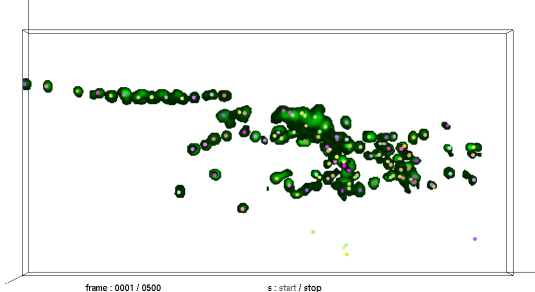
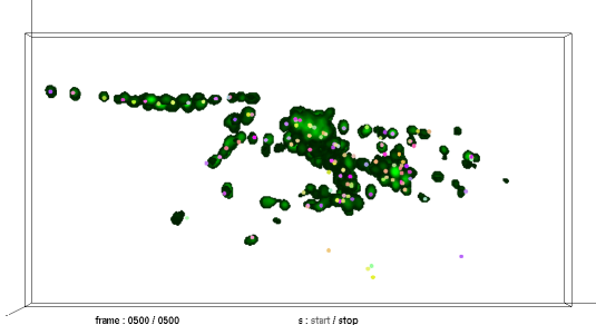
We evaluate tracking performance of SPF and the state-of-the-art method reported by Tokunaga et al.[23]. The data we used are D1, D2 and D3 in Data II reported by them, that is, 4D live-cell imaging data obtained by imaging nuclei of C. elegans neurons (Supplementary video 4-6). Each of the datasets is composed of 500 frames of 3D images with resolution $512\times 256\times 20$, i.e., 20 $z$-slices of 2D images with resolution $512\times 256$. Since the background noise level of the datasets changes according to the depth of the 3D image, we approximately estimated the background noise level as the average over fluorescent intensities of a 2D image and subtracted it from the 2D image. We then applied the median filter with window size $3\times 3\times 1$ to remove the salt-and-pepper noise. To obtain tracking results independent from the quality of cell detection, we used the same starting positions for the both methods. The starting positions were obtained by using the repulsive hill-climbing (RPHC) algorithm [23]. All the parameters required for SPF were manually-tuned and the same parameters were used for all of the three imaging data. The parameter set used for SPF and the resulting tracking animations of SPF (Supplementary video 7-9) and [23] (Supplementary video 10-12) are available in the supplementary website. Figure 3 shows tracking results of the both methods in the final frame of D3 in Data II. The top panel of the figure shows the starting positions of trackers. Five trackers that do not track cell centroids in the bottom of the image space are derived from false positives of cell-detection in the initial frame. The middle and bottom panels in Figure 3 show positions of trackers in the final frame for [23] and SPF, respectively. The figure suggests that at least large inconsistencies between cell centroids and positions of trackers for the both methods do not exist.

We evaluated tracking performance using the final frame of original datasets by manual verification. To reduce errors of manual verification as much as possible, we implemented following features for our 4D image viewer: (1) focusing only one cell and the corresponding tracker, (2) starting and stopping at an arbitrary frame, (3) rotation of the 4D image, and (4) adjustment of the intensity threshold that determines whether or not a voxel is displayed. These features of the 4D image viewer are introduced in Supplementary video 13. By using the features of our 4D image viewer, we calculated success rates of the both methods based on the following principles:

• A tracker was counted as success if the distance from the corresponding cell centroid was within $5$ voxels.

• A tracker was excluded from the calculation if it was an incorrectly detected cell centroid in the initial frame.

• A tracker was also excluded from the calculation if the corresponding cell centroid was out of view in the final frame.

Table 2 shows the success rates of the both methods based on the manual verification. SPF considerably improved tracking performance comparing with [23] for all the three datasets D1-D3 in Data II. Among the three datasets, tracking performance in D3 was noticeably lower than the other datasets for the both methods. This derives from the differences of nematodes’ body postures and movements in the final frame. The body postures in the final frame of D1 and D2 are roughly straight and movements of the nematode are moderate (Supplementary video 4 and 5). On the contrary, the nematode in the final frame of D3 is largely shrunk along the anterior-posterior axis and the nematode’s movement is rapid (Supplementary video 6).

Figure 3: Comparison of tracking performance for D3 in DATA II. (Top) Starting positions of trackers for the both methods. Trackers are depicted by colored circles. (Middle) Tracking result of [23] in the final frame. (Bottom) Tracking result of SPF in the final frame.

Table 2: The rate of trackers which correctly tracked corresponding cells in the final frame $t=500$ for D1-D3 in Data II. The number of cells in the initial frame detected by the RPHC algorithm is shown in parentheses of the first column. Consistency of tracking between the initial and final frames was manually checked for each cell using our 4D image viewer.

Data	Tokunaga et al. (2014)	SPF
D1 (120)	0.8000	0.9524
D2 (124)	0.6860	0.9669
D3 (111)	0.4467	0.8679

3.2 Comparison of cell-detection performance

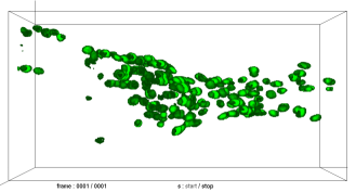
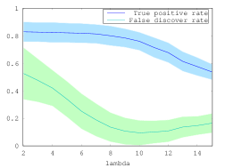
Next, we evaluate detection performance of the DP-means algorithm by comparing that of RPHC algorithm [23]. The datasets we use are DATA I reported by them. DATA I was obtained by imaging nuclei of nematode’s neurons likely to DATA II but is different in that (1) it is composed of distinct 3D still images instead of 4D images and (2) cell centroids were manually annotated in order to obtain the ground truth of the cell-detection problem. The resolution of $xy$-plane of all the ten datasets is $512\times 256$ and the numbers of $z$-slices for the datasets range from $119$ to $203$. A 3D image in Data I after the noise removal is shown in Figure 4. To evaluate the performance of the both algorithm, we counted the number of true positives (TP), the number of false positives (FP), and the number of false negatives (FN). A position detected by an algorithm is called a true positive if the position is within 5 voxels from a manually identified position, and is called a false positive otherwise. An annotated position that is not detected by an algorithm is called a false negative. We then computed true positive rates and false discovery rates defined as TP/(TP+FN) and FP/(FP+TP), respectively. Table 3 shows false discovery rates and true positive rates of the both algorithms. The radius parameter $\lambda$ of the DP-means algorithm was set to $8$ voxels close to the maximum radius of cells. The true positive rate of the DP-means algorithm is roughly the same as RPHC while its false discovery rate were higher than RPHC. Figure 5 shows an effect of the radius parameter $\lambda$ on cell-detection performance of the DP-means algorithm, suggesting that the DP-means algorithm achieved the best for $\lambda=8$ and $\lambda=9$ that are close to the maximum size of cells.

Figure 4: A 3D still image in DATA I that captured nuclei of C. elegans neurons after noise removal.

Table 3: False discovery rate and true positive rate of cell detection.

	RPHC	DP-means ($\lambda=8$)
True positive rate	0.8041 (0.0362)	0.8004 (0.0710)
False discovery rate	0.0301 (0.0305)	0.1362 (0.1060)

Figure 5: The radius parameter $\lambda$ and cell-detection performance of the DP-means algorithm. The accuracy was averaged over results of ten 3D still images in DATA I. Ranges within one standard deviation are indicated by shaded regions.

3.3 Computational Time

We computed CPU time and real time for D1 in DATA II that is composed of $500$ frames of 3D images with resolution $512\times 256\times 20$. We used iMac ($27$-inch, Late $2013$, OS X $10.9.5$) with $3.2$GHz Intel Core i$5$ and $8$GB RAM as our computational environment. OpenMP implemented in GCC 4.8 was used as a tool of parallelization. We used the same parameter set as that used in the evaluation of tracking performance for real 4D live-cell imaging data. Especially, we set the number of particles for tracking a cell to $1000$, i.e. the total number of particles for tracking $100$ cells is $10^{5}$. To measure the scalability of our method, we randomly selected $20,40,60,80$, and $100$ cells without replacement among $114$ cells. Figure 6 shows CPU time and real time consumed for tracking $500$ frames in the dataset D1 in DATA II. The CPU time and real time was averaged over $20$ trials. The CPU time in the most severe condition i.e. $K=100$ was less than 120 seconds, suggesting that our software is sufficiently of practical use.

Figure 6: The average time consumption of SPF and its scalability to the number of targets. CPU time and real time were evaluated for completing tracking of all $500$ frames of the dataset D1 in DATA II.

Discussion

We here summarize the results suggested by the numerical studies.

• The tracking performance of the standard PF was substantially improved by the proposed method for synthetic datasets (Table 1).

• The tracking errors of PF were sequentially inherited by the next frame, while that of SPF was not severely inherited. This result suggests a recovery from tracking failures (Figure 2).

• Tracking performance can be evaluated by using the features implemented in our 4D image viewer (Supplementary video 13).

• SPF considerably outperformed Tokunaga et al. in terms of success rates of tracking in the final frame for all the three datasets D1-D3 in Data II (Table 2).

• Parameters of SPF were set to the same ones for all the three datasets D1-D3 in DATA II, suggesting a robustness of SPF (Section 3.1).

• For the method of Tokunaga et al., some trackers were merged with other trackers and did not return to cells to be tracked again (Supplementary video 10-12).

• For SPF, some trackers often recovered from tracking failures and merged trackers were rarely observed, probably due to the integration of spatial information such as covariation, relative positions, and collision avoidance among cells (Supplementary video 7-9).

• True positive rates of the DP-means algorithm and the RPHC algorithm for detecting cell-centroids were roughly the same while the false positive rate of the DP-means algorithm was higher than that of the RPHC algorithm. This suggests an advantage of the RPHC algorithm over the DP-means algorithm for the detection of cell centroids (Table 3).

• The CPU times of SPF was proportional to the number of targets, suggesting a favorable property in terms of the scalability to the data size. (Figure 6).

4 Conclusion

In this study, we aimed at tracking of more than a hundred of cells in 4D live-cell imaging data. One important characteristic of live-cell imaging data is that cells to be tracked are densely scattered and visually similar. For these imaging data, the particle filter often mistakes a cell of interest for the other cells, since visual similarity among cell nuclei makes their discrimination difficult. Fortunately, our 4D live-cell imaging data shares a characteristic that is useful for accurate tracking: cells’ moves in the 4D live-cell imaging data are strongly correlated and the relative positions among target cells are roughly conserved.

To address the tracking issue, we designed an MRF that models the covariation and preservation of relative positions among cells. To avoid the inefficiency of JPF and MCMC sampling, we also proposed a novel sampling algorithm which we call spatial particle filter. The proposal distribution in the prediction step draws more accurate particles than those generated by dynamics since the proposal distribution shares both temporal and spatial information of a cell’s moves. SPF tracks cells by a sweep of an MRF tree in the spatial order for each frame; this allows effective simultaneous tracking. The MRF tree is automatically constructed by computing an MST among the initial locations of all targets. We applied the proposed method to synthetic data and our 4D live-cell imaging data of C. elegans. The results showed that our advantage over our previous algorithm.

Future work includes performance comparisons with tracking methods such as detection-and-linking and contour-evolution methods. Another direction is to expand the applicability of SPF to a wider class of 4D imaging data, for example, 4D images of chromosome arrangements during cell division. Tracking chromosomes is a challenging problem since they duplicate, split, and change their shapes according to the state of cell division. We expect the proposed method to be a reasonable candidate for tracking multiple targets in a wider class of 4D live-cell images.

Appendix

The source codes of SPF-CellTracker are available at the following github repository (S1). All the supplementary videos 1-13 described in Expeiriments section are available at the following supplementary website (S2). (S1) https://github.com/ohirose/spf (S2) https://sites.google.com/site/webosamuhirose/spf

Conflict of interest

None declared.

References

- [1] O. Al-Kofahi et al., Automated cell lineage construction: a rapid method to analyze clonal development established with murine neural progenitor cells. Cell Cycle, 5(3), 327–335, 2006.
- [2] N. Chenouard et al. Objective comparison of particle tracking methods. Nature methods, 11(3), 281–289, 2014.
- [3] N. Chenouard et al., Multiple hypothesis tracking for cluttered biological image sequences. IEEE Trans. Pattern Anal. Mach. Intell., 35, 2736–2750, 2013.
- [4] D. Clark et al., Temporal activity patterns in thermosensory neurons of freely moving Caenorhabditis elegans encode spatial temporal gradients. Journal of Neuroscience, 27(23), 6083–6090, 2007.
- [5] J. Deutscher et al., Articulated body motion capture by annealed particle filtering. Proceedings of IEEE Conference on Computer Vision and Pattern Recognition, 2, 126–133, 2000.
- [6] A. Doucet et al., On sequential Monte Carlo sampling methods for Bayesian filtering. Statistics and Computing, 197–208.
- [7] A. Dufour et al., 3-D active meshes: fast discrete deformable models for cell tracking in 3-D time-lapse microscopy. IEEE Trans. Image Process., 20(7), 1925–1937, 2011.
- [8] C. Gomila, Graph-based object tracking. Proceedings of the International Conference on Image Processing, 2, 41–44, 2003.
- [9] R.E. Kalman, A new approach to linear filtering and prediction problems. J. Fluids Eng., 82(1), 35–45, 1960.
- [10] Z. Khanet al., An MCMC-based particle filter for tracking multiple interacting targets. Proceedings of the 8th European Conference on Computer Vision, 279–290, 2004.
- [11] J.B. Kruskal, On the shortest spanning subtree of a graph and the traveling salesman problem. Proceedings of the American Mathematical Society, 7(1), 48–50, 1956.
- [12] B. Kulis et al., Revisiting k-means : new algorithms via Bayesian nonparametrics. Proceedings of the 29th International Conference on Machine Learning, 513–520, 2012.
- [13] F. Liet al. Multiple nuclei tracking using integer programming for quantitative cancer cell cycle analysis. IEEE Trans. Med. Imaging, 29(1), 96-105, 2010.
- [14] F. Li,et al. Cell population tracking and lineage construction with spatiotemporal context. Med. Image Anal., 12(5), 546-566, 2008.
- [15] H.T. Chenet al., Multi-object tracking using dynamical graph matching. Proceedings of the IEEE Computer Society Conference on Computer Vision and Pattern Recognition, 2, 210–217, 2001.
- [16] E. Meijeringet al., Methods for cell and particle tracking., Methods Enzymol., 504(9), 183–200, 2012.
- [17] K. Nummiaroet al., Object tracking with an adaptive color-based particle filter. Pattern Recognition, 353–360, 2002.
- [18] Y. Ruiet al., Better proposal distributions: object tracking using unscented particle filter. Proceedings of the IEEE Computer Society Conference on Computer Vision and Pattern Recognition, 2, 786–793, 2001.
- [19] T. Schrödelet al., Brain-wide 3D imaging of neuronal activity in Caenorhabditis elegans with sculpted light. Nature methods, 10, 1013–1020, 2013.
- [20] M. Maška et al., Segmentation and shape tracking of whole fluorescent cells based on the Chan-Vese model. IEEE Trans. Med. Imaging, 32, 995–1006. 2013.
- [21] M. Maška et al., A benchmark for comparison of cell tracking algorithms. Bioinformatics, 30(11), 1609–1617, 2014.
- [22] I. Smal, et al., Rao-Blackwellized marginal particle filtering for multiple object tracking in molecular bioimaging. Proceedings of the International Conference on Information Processing in Medical Imaging, 20, 110–121, 2007.
- [23] T. Tokunagaet al., Automated detection and tracking of many cells by using 4D live-cell imaging data Bioinformatics, 30, i43–i51.
- [24] J. Vermaaket al., Maintaining multimodality through mixture tracking. Proceedings of the 9th IEEE International Conference on Computer Vision, 2, 1110–1116, 2003.
- [25] J. Wanget al., Online selecting discriminative tracking features using particle filter. Proceedings of the IEEE Conference on Computer Vision and Pattern Recognition, 2, 1037–1042, 2005.
- [26] K. Yamadaet al., Olfactory plasticity is regulated by pheromonal signaling in Caenorhabditis elegans. Science, 329(5999), 1647–1650, 2010.
- [27] K. Yoshidaet al., Odour concentration-dependent olfactory preference change in C. elegans. Nature communications, 3, 739, 2012.
- [28] Y. Zhaoet al., An expanded palette of genetically encoded indicators. Science, 333(6051), 1888–1891, 2011.