Decoherence of Einstein-Podolsky-Rosen steering
Abstract
We consider two systems and that share Einstein-Podolsky-Rosen (EPR) steering correlations and study how these correlations will decay, when each of the systems are independently coupled to a reservoir. EPR steering is a directional form of entanglement, and the measure of steering can change depending on whether the system is steered by , or vice versa. First, we examine the decay of the steering correlations of the two-mode squeezed state. We find that if the system is coupled to a reservoir, then the decoherence of the steering of by is particularly marked, to the extent that there is a sudden death of steering after a finite time. We find a different directional effect, if the reservoirs are thermally excited. Second, we study the decoherence of the steering of a Schrodinger cat state, modelled as the entangled state of a spin and harmonic oscillator, when the macroscopic system (the cat) is coupled to a reservoir.
OCIS: 270.0270; 270.6570; 270.5568
I Introduction
The sort of nonlocality we call “Einstein-Podolsky-Rosen-steering” Schrodinger ; key-2 ; hw-steering-1 ; hw2-steering-1 ; EPRsteering-1 ; eprsteerphoton-1 originated in 1935 with the Einstein-Podolsky-Rosen (EPR) paradox epr . The EPR paradox is the argument that was put forward by Einstein, Podolsky and Rosen for the incompleteness of quantum mechanics. The argument was based on premises (sometimes called Local Realism or in Einstein’s language, no “spooky action-at-a-distance”) that were not restricted to classical mechanics, but were thought essential to any physical theory bell book . The EPR argument reveals the inconsistency between Local Realism and the completeness of quantum mechanics. It does not in itself rule out all completions of quantum mechanics, that are compatible with local realism. Nowadays, after the work of Bell, we realise this ruling out of all local realistic theories can be done in some special experimental situations Bell ; key-4 ; bellloophole ; key-3 . Any realisation of the EPR paradox wuepr ; rmp-1 ; ou , as a special case of EPR steering, is nonetheless important in giving a concrete intermediate result: the fact that quantum mechanics without completion cannot be consistent with local realism. A great advantage of EPR-steering over Bell-type tests is that they are more accessible to mesoscopic or macroscopic systems. EPR steering tests have been quantitatively studied or proposed for optical down conversion ou ; mdrdrumm ; rmp-1 ; mdrepr-1 , optical systems in nonlinear regimes near or at critical points karl , atomic gas ensembles at room temperature polzik room temp ; thermal atomic ensembles ; key-5 , Bose-Einstein condensates (BEC) eprbecobert ; karenbec ; beceprbargill ; key-6 ; key-7 ; key-8 ; ferriseprbec ; prlobertbec ; key-9 ; key-10 , and opto-mechanics simon ; opto ; paoloepr ; thermal he andR . This may lead to experimental tests of Schrodinger cat-type states.
The EPR paradox manifests as a strong correlation between the positions and momenta of two spatially separated particles (or some equivalent correlations). These correlations, once one assumes Local Realism, become inconsistent with the uncertainty principle. Given the strangeness of the EPR correlations, a likely hypothesis would be that they do not exist in real physical systems. Indeed, the sort of correlations needed for EPR are not easily realisable in experiment. To date, only a few experiments can justify the claim of loophole-free EPR correlations witt NJP zeilloopholefree-1 , or steering without detection efficiency loopholes loopholesteer ; smith UQ steer -1 ; ou ; rmp-1 . This paper examines why this is so: There are two possibilities.
(1) It could be that quantum mechanics needs modification to the extent that EPR correlations cannot be predicted. If we accept irrefutable evidence now exists for EPR correlations, then this probability would appear falsified. However, we comment that the experimental realisations for EPR steering have been for optical systems, not yet for atoms or mesoscopic devices.
(2) Or else: a popular belief is that quantum mechanics is correct as it is, and predicts exactly why, to a great accuracy, the EPR correlations are extraordinarily difficult to measure. In that case, these predictions need to be evaluated and verified by experiment.
This last point is what we examine in this paper: We study in detail why, according to quantum predictions, the EPR correlations are not easily realisable. As with the well known “Schrodinger cat” schcat ; key-14 ; catstrappedions ; key-11 ; singlemodecat ; cats ; cats3 ; yurke stoler ; key-12 ; key-13 , we expect this is so, because of the effect that occurs when a quantum system is coupled to its environment, modelled as a large system - a reservoir legdecoh . This effect is called “decoherence”.
Here, we examine some different sorts of decoherence that occur for EPR steering. As with the decay of entanglement, there are many cases one can study. It is worth noting that EPR steering was realised using high efficiency detection for optical amplitudes ou ; rmp-1 , and has also been unambiguously detected in photonic scenarios with exceptional losses () loopholesteer . Tests have also begun for its genuine multipartite form, distributed among different locations seijigen ; key-17 ; key-15 ; key-16 .
In this paper, we restrict our investigation to the following cases: We study position-momentum measurements or their optical equivalent, quadrature phase amplitude measurements. First, we analyze the steering of a two-mode squeezed state, to understand the decoherence effects of coupling to a thermal reservoir. We examine two properties of the decoherence: the effect of simple losses (damping); and the effect of thermal noise. Second, we consider a special case of EPR-steering, that relates to a macroscopic/mesoscopic superposition state - a “Schrodinger cat” state. In fact, the EPR-steering paradox can be used to signify the Schrodinger cat superposition erci cav reid pra . We examine the effect of decoherence as caused by interaction with the environment, on this signature.
An interesting new feature evident for EPR-steering is that the nonlocality can manifest asymmetrically with respect to the observers steer thmurray ; brunner ; onewaysteer ; eprsteer-1 ; asymmschnee ; monog . In our results, we focus on the asymmetry of the decoherence effects on the EPR-steering. This is valuable to understand, not only from the fundamental perspective of testing quantum mechanics, but from the point of view of the potential applications of EPR-steering, which include cryptography epr crypto ; norbet ; key-18 ; key-19 ; onesided ; grangiertele and no-cloning teleportation grangiertele . One-sided device-independent cryptography has been proposed using EPR steering inequalities onesided . In recent papers, it was shown how the asymmetric effects of loss on EPR-steering could affect the optimal location of teleportation stations tele , or which entanglement criterion should be used to faithfully verify entanglement in cases of untrusted devices onesided ; onesidedbog ; grangiertele ; norbet ; tele .
II Decoherence of steering for the two-mode squeezed state
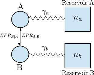
Consider two quantum harmonic oscillators, with boson operators and , and depicted in the Figure 1 as systems and . Such oscillators can be coupled, so that EPR-steering correlations are induced between the two oscillators.
One of the nicest examples of such EPR steering has been realised experimentally in optics rmp-1 as the two-mode squeezed state tmss-1 . Here, each mode of the light field is modeled as a quantum harmonic oscillator. An example of a coupling between the oscillators that generates this type of state is called parametric down conversion, and can be described by the interaction Hamiltonian in an appropriate rotating frame mdrepr-1
| (1) |
Similar two-mode squeezed states can be generated by impinging two single-mode squeezed states into the two different input ports of an optical beam splitter tele-1 .
The two-mode squeezed state system is fundamentally interesting, as it can be quite accurately realised in optics, but also it gives a reasonable approximation to the effects we expect to see in many other physical realisations of steering, such as in opto-mechanics opto ; thermal he andR ; simon , atomic ensembles polzik room temp ; thermal atomic ensembles ; key-5 , and BEC eprbecobert ; beceprbargill ; key-6 ; key-7 ; key-8 ; ferriseprbec ; prlobertbec ; key-9 ; key-10 . The study of the effect of the thermal environment on the EPR steering for a two-mode squeezed state will therefore give us insight into a broad set of physical scenarios. The two-mode quantum correlation effects were noticed originally in the context of photon number correlations between the two beams, which gives rise to noise reduction heidmann-1 ; key-20 .
II.1 The two-mode squeezing Hamiltonian
We begin by reviewing the solution for the EPR correlations given by the Hamiltonian of Eq. (1). The EPR solutions were originally derived in mdrepr-1 . We define the quadrature phase amplitudes , , and for each mode: and . This choice of scaling for the amplitudes will imply the Heisenberg uncertainty relations and . We note that depending on the physical system modelled by the Hamiltonian, the amplitudes can also correspond to scaled position and momentum observables. We now ask what correlations are generated between the quadrature amplitudes, after an interaction time between the two modes, at sites denoted by and .
On examining (1), the resulting coupled equations for and can be readily solved, to give
| (2) |
where . We define the squeezing parameter as . The quadrature phase amplitudes are given by
| (3) |
This enables us to calculate correlations such as , after a time , assuming initial uncorrelated vacuum states for all modes. We can then evaluate the variance of , which will be denoted and which equals when we assume vacuum inputs at . We have introduced constants , which can be chosen to minimise the variance relative to the Heisenberg quantum noise level of the amplitudes and . We find this value of by standard procedures mdrepr-1 ; rmp-1 :
| (4) |
For the system described by the Hamiltonian of Eq. (1), we find the optimal value is . The optimal variance is given by:
| (5) |
which for the parametric system (1) becomes . Similarly we evaluate the variance of , which we will denote as : The variance minimizes when
This optimal value of for system (1) is The optimal variance is given by
| (6) |
which becomes for Eq. (1).
II.2 EPR steering correlations
The criterion for the EPR paradox introduced in mdrepr-1 is also a criterion for EPR steering EPRsteering-1 ; hw-steering-1 ; hw2-steering-1 . This EPR steering criterion is defined as the square root of the variance product:
| (7) |
We observe EPR steering (of system by ) whenever
| (8) |
The ideal correlations created by the parametric down conversion Hamiltonian interaction (1) are obtained in the limit of and correspond to the EPR variances becoming zero, and hence .
The EPR steering condition (8) by its very definition will negate all local hidden state (LHS) models of the type hw-steering-1 ; hw2-steering-1
| (9) |
These LHS models are similar to the local hidden variable models introduced by Bell Bell ; key-3 . Here represents hidden variable parameters and is the probability distribution for these parameters. The is independent of the choice of measurement ( and ), which is made after the generation and separation of the subsystems and . In this model, the is the average value for the result , given the hidden variable state specified by . The is defined similarly. For the LHS model however, there is the additional asymmetrical constraint that the local hidden variable moments (such as ) for system be consistent with measurements of some local observables (for example position and momentum) at , and is thus able to be described as arising from a local quantum density operator .
II.3 Reservoir coupling
We now examine the effect on EPR steering if the systems and are independently coupled to heat bath reservoirs (Figure 1). We assume that the parametric interaction given by (1) that generates a two-mode squeezed state is turned off at the time , and the system left to decay. The two-mode squeezed state is a so-called Gaussian state, meaning that its characteristic function is Gaussian gauss . Within the constraint of two-mode Gaussian states and measurements, the condition (8) will provide a necessary and sufficient test of steering hw-steering-1 ; hw2-steering-1 . This makes the criterion valuable, for understanding the effects of decoherence in Gaussian systems.
Thus, we consider a system prepared in a two-mode squeezed state at time . In principle, the modes and can be spatially separated. We consider the coupling of each mode and to independent heat baths (reservoirs) with thermal occupation numbers and respectively. The solutions after coupling to the reservoir are straightforward to evaluate using the operator Langevin equations that describe the evolution of the mode operators crispn paper ; key-21 :
| (11) |
Here and describe the decay rates (losses) that are induced by the reservoirs. The quantum reservoir operators have nonzero correlations given by and where the numbers and give the level of thermal occupation of the reservoirs. Solutions are
| (12) |
From this, we can calculate the moments at a later time, in terms of the initial moments:
| (13) |
The solution for is obtained from that for , but exchanging the letters with . The initial moments are given by the solutions found in Section II.A. The final moments after reservoir coupling are
| (14) |
The covariance matrix is defined as:
| (15) |
Hence we find , , , , where
| (16) |
Applying the results of the Section II.A, we calculate that
| (17) |
II.4 Decoherence of EPR steering with no thermal noise
We first assume negligible thermal noises: we put in the solution given by Eq. (17). The decoherence effect on the system by the reservoirs manifests as losses, parametrised by and . We will study the effect on the steering parameters, showing the effect of loss to be asymmetrical with respect to the two systems and .
II.4.1 Damping the steering system: Steering sudden-death
Let us suppose that the reservoirs are coupled asymmetrically, so that i.e. only the mode is coupled to a reservoir. In this case, we find for the steering of (mode )
| (18) |
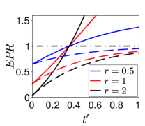
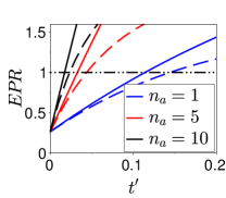
The plots of Figure 2 (left graph) indicate that where the losses are entirely on the steering mode , the decoherence of EPR steering is substantial. After a time given by , steering (as measured by ) in that direction is lost. The loss is inevitable, regardless of how much steering is present in the initial two-mode quantum system, as shown by the results for the different values of squeeze parameter : We also note that the cut-off time for steering is independent of the amount of steering in the initial two-mode system. The behavior observed here is analogous to the “entanglement sudden-death”, that has been observed for the decoherence of entanglement eberly ; key-23 ; key-22 .
II.4.2 Damping the steered system
However, the sudden-death effect is not apparent when the “steered” system is lossy. We again assume and evaluate the steering of the damped system, by the undamped system:
| (19) |
The plots of Figure 2 (left graph) reveal the nature of the decoherence when only the steered system is damped. Here, we see that there is much less sensitivity of the steering to the losses. In fact, while the EPR steering is certainly diminished by the dissipation, there is no cut-off, or sudden death, but rather steering is still possible for arbitrary times, . We remark that the increased sensitivity to losses affecting the steering system, as compared to the steered system, has been noted in earlier papers rmp-1 ; onewaysteer ; steer thmurray ; monog .
II.4.3 Symmetric decoherence
We next consider a reservoir with symmetric damping .
| (20) | |||||
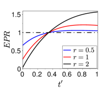
The results of Figure 2 (right graph) show, as might be expected, the effect is dominated by the fact that the steering system is damped. Here steering (as measured by ) is also lost at .
II.5 Decoherence of EPR steering with thermal noise
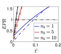
Now we consider the more complex interaction where there is additional thermal noise for each reservoir. Here we use the full expressions given by Eq. (17). Our results in Figures 3 and 4 reveal several features. We note that the loss of steering is rapid and complete (“sudden-death”) if the thermal noise is placed on the system that is being steered. This effect has been noticed in previous studies of thermal steering and is especially important for asymmetrical systems such as found in opto-mechanics simon ; thermal he andR ; karenbec ; thermal atomic ensembles . The effect is more significant as the thermal noise increases, but is reduced for higher (Figure 4).
II.6 Comparing with the decoherence of entanglement
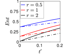

The effects of the reservoir on the steering are asymmetrical. This will not be true for entanglement: Entanglement is symmetrically defined, with respect to the two different systems involved, and the numerical value we assign to the entanglement will be unchanged under the exchange . The relationships between entanglement and EPR steering for Gaussian states have been recently studied prlgaussadesso ; key-24 . For Gaussian states, it is possible to give a quantification of steering prlgaussadesso ; hw-steering-1 ; hw2-steering-1 ; key-24 , which is an asymmetrical quantum correlation, similar to quantum discord prlstefano ; key-32 ; key-31 .
We may evaluate the entanglement via the parameter itent ; key-33 . The inequality is a necessary and sufficient condition for entanglement of two-mode Gaussian systems for the case we examine here where . The condition for optimally chosen has been shown equivalent to the Peres-Simon condition in that case key-24 . Thus, in this section, we consider the entanglement parameter
| (21) |
First we find the value of that minimizes the parameter We evaluate , in this case we know that hence:
Next
Hence the value of that minimizes is key-24 :
We note that if , then the value of that minimises the expression is , but where we have asymmetric reservoir effects, like different reservoir couplings or thermal noises, the optimal value will be different to . Here we will use from Section II.A that:
Figure 5 plots the entanglement for various reservoir couplings. We see from Figure 5 (left graph) that where there is no thermal noise, the entanglement decays steadily, but is never destroyed completely. This effect was noted in buono bow ; key-34 . The larger values of correspond to larger amounts of entanglement for the initial state before decoherence, and we note that while the decay is sharper for higher , a larger initial amount of EPR entanglement will ensure larger EPR entanglement for all later times. The Figure 5 (right graph) shows that when the reservoirs are thermally excited, the entanglement is totally destroyed (in sudden-death fashion) after a finite time. This time is shortened, by increasing the amount of thermal excitation of the reservoir (on either system).
III Decoherence of the steerability of a S-cat state
Traditionally, most studies of decoherence have centred around the Schrodinger cat legdecoh ; yurke stoler ; key-12 ; key-13 ; key-14 . We noticed in the study of the decoherence of steering for the two-mode squeezed state that for stronger EPR effects, the decay was brought about more sharply, to give overall decoherence times of a similar order (Figure 2). This is consistent with the overall intuition about decoherence in quantum mechanics, that it acts to destroy the more extreme (larger) effects more quickly so that they are not observed in nature. This has been studied for the Schrodinger cat example, where one considers a system initially prepared in superposition of two states macroscopically distinguishable e.g. in phase space legdecoh ; cats ; cats3 ; yurke stoler ; key-12 ; key-13 ; key-14 . The coupling to a reservoir induces a decay of the superposition. Where the separation in phase space increases, calculation and experiments show that the decay rate will increase. Thus, there is an explanation of the transition from microscopic to macroscopic quantum mechanics. Here, motivated by this, we examine the decoherence of the EPR steering of a Schrodinger cat state.
III.1 Steering signature for a Schrodinger cat
Consider the state:
| (25) |
which is the entangled Schrodinger cat state. We select and to be real. Here, is the coherent state for mode of system and , are the eigenstates of the Pauli spin of system . This state is similar to that described in Schrodinger’s original gedanken experiment schcat , where a microscopic system becomes entangled with a macroscopic one, the “cat”. The spin-mode entangled state given by Eq. (25) has been the subject of several experiments cats . We first explain how one can signify the Schrodinger cat, using EPR steering.

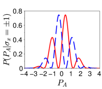
We will derive the probability distributions (or ) for the system , given that a measurement of the Pauli spin (or ) at has been carried out to give a result or . We define the scaled amplitudes for position and momentum by where is the boson operator, and note that for real position and momentum, . In terms of the quadrature phase amplitudes and defined in Section II, however, we chose the scaling . We will distinguish the two cases by using lower and upper case, respectively, and note we have dropped the use of the operator hats where the meaning is clear, or to denote the outcomes of the measurements. As expected from direct examination of the state (25), the distributions and for the result at given the outcomes or for at , are the two Gaussian hills (Figure 6, left graph): Specifically,
Next, we derive the conditional distributions for given that a measurement of Pauli spin at yields the result or . To evaluate this, we rewrite the state in terms of the basis states and for the spin .
| (27) | |||||
At this point, we note the for other choices of , normalisation factors are more complicated. We find that the probability for the momentum given the results for spin is
This allows us to calculate the conditional variances that give us a signature for steering. An EPR steering of the “cat” is observed when
| (29) |
where here
denotes the conditional variance for averaged over the outcomes of . We have used the notation to mean the variance of , which is the probability distribution for given the outcome for the measurement , respectively. The is defined similarly, but for outcomes of . The right-side bound is the quantum noise limit, as determined by the Heisenberg uncertainty relation which in this case for the choice is . We note that the derivation of the inequality as a signature of EPR steering has been given in the Refs. EPRsteering-1 ; mdrepr-1 ; rmp-1 .
The EPR quantity (29) can be evaluated: We see that for the two Gaussian hills, the variance is at the quantum noise level (Figure 6, left graph): . On the other hand, the variance associated with the momentum distributions is reduced below (Figure 6, right graph), implying that . We can calculate the variance from the conditional distributions. Alternatively, noting that the collapsed state for system given a measurement is the superposition (for result ) or (for result ), it is easy to use the methods and results of the next section, to find that
| (30) |
The steering inequality (29) has been suggested in Ref. erci cav reid pra , as a way to realise an EPR paradox with the Schrodinger cat state. The steering cannot be obtained if the system is in the mixture of states, and , that allows a classical dead or alive description. This case is especially interesting, because it focuses on the steering of a mesoscopic system (the Schrodinger cat) thermal he andR . If we assume Local Realism is valid, then it is the local state of the mesoscopic system that is shown to be inconsistent with the quantum mechanics (refer to the LHS model of the Section II.B). This contrasts with EPR’s original argument, which showed the inconsistency for a microscopic system epr .
III.2 Decoherence of the Schrodinger cat with a heat bath
It will prove useful to next study the interaction of the single mode “Schrodinger cat” state yurke stoler ; key-14 ; key-12 ; key-13
| (31) |
with a reservoir. This was analysed by many authors, including Yurke and Stoler yurke stoler ; legdecoh ; key-12 ; key-13 ; key-14 . We consider that the single mode, prepared in the Schrodinger cat state, is then coupled to a thermal heat bath with dissipation. Using the solutions from Section II.C, we can calculate the moments at a later time , in terms of the initial moments:
Denoting the variances using shorthand notation, by and , we find
| (32) |
We see that the variance for can be reduced below the quantum limit (given by ). The reduction of the variance of below the quantum limit is in itself a signature for the “cat” state. We see this as follows. If we take large, and assume no thermal noise and , then the probability distribution associated with each of the “dead” and “alive” states is a Gaussian hill, with variance . If the system were to actually be in any kind of mixture of these quantum states, then the variance for could not drop below because of the uncertainty relation (and the fact that mixing states cannot decrease the variance) erci cav reid pra ; prl eric . The observation of a reduced variance for can thus occur for a superposition but not for a mixture of the two quantum states that possess a distribution given by the Gaussian hills. The details are not studied further here however, since our objective is to study the decoherence of steering.

III.3 Decoherence of the steering of the Schrodinger cat
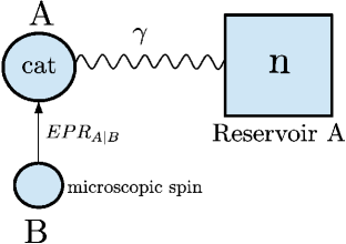
Motivated by this, we now examine the decoherence of the EPR steering of a Schrodinger cat state, as given by the signature Eq. (29). We consider the two-mode case where is a harmonic oscillator coupled to a heat bath from time and the second system is the spin (no heat bath coupling), as depicted in Figure 7. The system is prepared in the entangled Schrodinger cat state
| (33) |
We can rewrite this state in terms of the basis states and for the spin as shown in Section III.A. It is straightforward to calculate the moments , , etc. at the time . The moments at a later time (after the interaction with the heat bath has been turned on) can be evaluated using the solution (12) of Section II.C. We note that since the reservoir interaction does not involve the spins, we have , . Therefore, we can calculate the moments at the time , in terms of the moments at the initial time .
We next consider the moments of the distributions at the time for and , conditional on getting the result either or for the Pauli spin measurement on . These moments can be readily calculated. We outline the method. We use the notation, for example, to denote the moment of system conditioned on the result for spin at . Let us suppose then that we obtain the outcomes at , and at . We define the measurable probability for the joint outcomes. We see that: . It follows that . Hence, . Following this procedure, we see that:
| (34) |
and similarly for the moments involving . This allows us to solve for the conditional moments using the relations such as and . We also define the same relations, but replacing with and with . The final solutions for the conditional moments are: , , and . Hence we solve for the average variance of conditioned on the measurement of spin at : We obtain
| (35) |
Similarly, we can solve for variance of conditioned on spin at , to obtain
| (36) |
To show how the EPR steering signature decoheres with time, we evaluate
| (37) |
Here, we use the notation defined in Section III.A.
We find that with (no thermal noise), the value of is identical to that of which is also identical to the variance given by Eq. (32). This value is plotted in Figure 8 (solid lines). By the above argument, the signature of the S-cat is the drop below of . We note that as increases, the value tends to , the signature therefore becoming more sensitive to decoherence. This reduction in variance of as increases is directly associated with the interference fringes in the distribution yurke stoler ; key-14 ; key-12 ; key-13 . These fringes become finer as increases, as evident from the function given by Eq. (LABEL:eq:fringe5). With thermal noise, we see that the value of increases: a much greater sensitivity to decoherence is apparent, as illustrated in Figure 8 by the dashed-dotted curves.
IV Conclusion
The directional properties of EPR steering are significant when it comes to understanding the decoherence of EPR-steering. We have shown how when two systems are coupled independently to a reservoir, the steering is asymmetrically affected. If we consider the steering of a system by measurements made on the system , then the steering is sensitive to the reservoir coupling to system . This is intuitively not surprising, given the Local Hidden State (LHS) definition of EPR steering as a nonlocality. In terms of the LHS description that is to be negated in order to confirm such steering by B hw-steering-1 ; hw2-steering-1 , it is the hidden states of system that are like those considered by Bell. The sensitivity of the steering to the losses on the system has been studied experimentally, in the context of the EPR paradox buono bow ; erci cav reid pra ; key-34 . There, it was known that the EPR criterion could not be achieved, with or more losses on the steering system . Recent work considers this result in terms of the monogamy properties of EPR steering monog . The sensitivity of the steering signatures to losses (which may represent an eavesdropper on the channel) has potentially important implications for quantum cryptography onesided ; onesidedbog .
The behaviour with respect to the thermal noise appears almost reversed. This has implications for detecting steering of Schrodinger cats which are coupled to hot reservoirs. For the Schrodinger cat example, we explained how the steering acts as a signature of the Schrodinger cat. Adding thermal noise to the system significantly affects the amount of EPR steering of system . There have been recent theoretical studies of the steering of a mechanical oscillator, which we liken to a “cat”, by measurements made on an optical pulse thermal he andR ; simon . In those studies, the thermal noise of the oscillator was shown to have a quite dramatic effect on the amount of steering possible. By comparison, the entanglement between the thermal oscillator and the pulse was quite robust. Similar results have been obtained for Bose Einstein condensates karenbec . These results are consistent with the simple descriptions of decoherence given in this paper.
Acknowledgements.
This work was supported by an Australian Research Council Discovery Project Grant. We are grateful to B. Dalton for many helpful suggestions.References
- (1) E. Schroedinger, “Discussion of probability relations between separated systems,” Proc. Cambridge Philos. Soc. 31, 555-563 (1935).
- (2) E. Schroedinger, “Probability relations between separated systems ,” Proc. Cambridge Philos. Soc. 32, 446-452 (1936).
- (3) H. M. Wiseman, S. J. Jones, and A. C. Doherty, “Steering, entanglement, nonlocality, and the Einstein-Podolsky-Rosen paradox,” Phys. Rev. Lett. 98, 140402 (2007).
- (4) S. J. Jones, H. M. Wiseman, and A. C. Doherty, “Entanglement, Einstein-Podolsky-Rosen correlations, Bell nonlocality, and steering,” Phys. Rev. A 76, 052116 (2007).
- (5) E. G. Cavalcanti, S. J. Jones, H. M. Wiseman, and M. D. Reid, “Experimental criteria for steering and the Einstein-Podolsky-Rosen paradox,” Phys. Rev. A 80, 032112 (2009).
- (6) D. J. Saunders, S. J. Jones, H. M. Wiseman, and G. J. Pryde, “Experimental EPR-steering using Bell-local states,” Nature Physics 6, 845-849 (2010).
- (7) A. Einstein, B. Podolsky and N. Rosen, “Can quantum-mechanical description of physical reality be considered complete?,” Phys. Rev. 47, 777-780 (1935).
- (8) J. S. Bell, “Speakable and unspeakable in quantum mechanics” (Cambridge University Press, Cambridge, 1987).
- (9) J. S. Bell, “On the Einstein-Podolsky-Rosen paradox,” Physics 1, 195-200 (1964).
- (10) J. F. Clauser, M. A. Horne, A. Shimony, and R. A. Holt, “Proposed experiment to test local hidden-variable theories,” Phys. Rev. Lett. 23, 880-884 (1969).
- (11) M. Giustina, A. Mech, S. Ramelow, B. Wittmann, J. Kofler, J. Beyer, A. Lita, B. Calkins, T. Gerrits, S. W. Nam, R. Ursin, and A. Zeilinger, “Bell violation using entangled photons without the fair-sampling assumption,” Nature 497, 227-230 (2013).
- (12) B. G. Christensen, K. T. McCusker, J. B. Altepeter, B. Calkins, T. Gerrits, A. E. Lita, A. Miller, L. K. Shalm, Y. Zhang, S. W. Nam, N. Brunner, C. C. W. Lim, N. Gisin, and P. G. Kwiat, “Detection-loophole-free test of quantum nonlocality, and applications,” Phys. Rev. Lett. 111, 130406 (2013).
- (13) C. S. Wu, and I. Shaknov, “The angular correlation of scattered annihilation radiation,” Physical Review A 77, 136 (1950).
- (14) Z. Y. Ou, S. F. Pereira, H. J. Kimble, and K. C. Peng, “Realization of the Einstein-Podolsky-Rosen paradox for continuous variables,” Phys. Rev. Lett. 68, 3663-3666 (1992).
- (15) M. D. Reid, P. D. Drummond, W. P. Bowen, E. G. Cavalcanti, P. K. Lam, H. A. Bachor, U. L. Andersen, and G. Leuchs, “Colloquium: The Einstein-Podolsky-Rosen paradox: From concepts to applications,” Rev. Mod. Phys. 81, 1727-1751 (2009).
- (16) M. D. Reid, “Demonstration of the Einstein-Podolsky-Rosen paradox using nondegenerate parametric amplification,” Phys. Rev. A 40, 913-923 (1989).
- (17) M. D. Reid, and P. D. Drummond, “Quantum correlations of phase in nondegenerate parametric oscillation,” Phys. Rev. Lett. 60, 2731-2733 (1988).
- (18) K. Dechoum, S. Chaturvedi, P. Drummond, and M. D. Reid, “Critical fluctuations and entanglement in the nondegenerate parametric oscillator,” Phys. Rev. A70, 053807 (2004).
- (19) B. Julsgaard, A. Kozhekin, and E. S. Polzik, “Experimental long-lived entanglement of two macroscopic objects,” Nature 413, 400-403 (2001).
- (20) H. Krauter, C. A. Muschik, K. Jensen, W. Wasilewski, J. M. Petersen, J. I. Cirac, and E. S. Polzik, “Entanglement generated by dissipation and steady state entanglement of two macroscopic objects,” Phys. Rev. Lett. 107 080503 (2011).
- (21) Q. He, and M. Reid, “Towards an Einstein–Podolsky–Rosen paradox between two macroscopic atomic ensembles at room temperature,” New J. Phys., 15, 063027 (2013).
- (22) C. Gross, H. Strobel, E. Nicklas, T. Zibold, N. Bar-Gill, G. Kurizki, and M. K. Oberthaler, “Atomic homodyne detection of continuous-variable entangled twin-atom states,” Nature 480, 219-233 (2011).
- (23) N. Bar-Gill, C. Gross, I. Mazets, M. Oberthaler, and G. Kurizki, “Einstein-Podolsky-Rosen correlations of ultracold atomic gases,” Phy. Rev. Lett, 106, 120404 (2011).
- (24) K. Kheruntsyan, M. Olsen, and P. D. Drummond, “Einstein-Podolsky-Rosen correlations via dissociation of a molecular Bose-Einstein condensate,” Phys. Rev. Lett. 95, 150405 (2005).
- (25) M Ögren, and K. V. Kheruntsyan, “Role of spatial inhomogeneity in dissociation of trapped molecular condensates,” Phys. Rev. A 82, 013641 (2010).
- (26) J. Jaskula, M. Bonneau, G. B. Partridge, V. Krachmalnicoff, P. Deuar, K. V. Kheruntsyan, A. Aspect, D. Boiron, and C. I. Westbrook, “Sub-Poissonian number differences in four-wave mixing of matter waves,” Phys Rev. Lett. 105, 190402 (2010).
- (27) A. Ferris, M. Olsen, E. Cavalcanti, and M. Davis, “Detection of continuous variable entanglement without coherent local oscillators,” Phys. Rev. A 78, 060104 (2008).
- (28) Q. He, M. Reid, T. Vaughan, C. Gross, M. Oberthaler, and P. Drummond, “Einstein-Podolsky-Rosen entanglement strategies in two-well Bose-Einstein condensates,” Phys. Rev. Lett. 106, 120405 (2011).
- (29) Q. He, P. Drummond, M. Olsen, and M. D. Reid, “Einstein-Podolsky-Rosen entanglement and steering in two-well Bose-Einstein-condensate ground states,” Phys. Rev. A 86, 023626 (2012)
- (30) B. Opanchuk, Q. He, M. Reid, and P. Drummond, “Dynamical preparation of Einstein-Podolsky-Rosen entanglement in two-well Bose-Einstein condensates,” Phys. Rev. A 86, 023625 (2012).
- (31) R. J. Lewis-Swan, and K. V. Kheruntsyan, “Sensitivity to thermal noise of atomic Einstein-Podolsky-Rosen entanglement,” Phys. Rev. A 87, 063635 (2013).
- (32) S. G. Hofer, W. Wieczorek, M. Aspelmeyer, and K. Hammerer, “Quantum entanglement and teleportation in pulsed cavity optomechanics,” Phys. Rev. A 84, 052327 (2011).
- (33) V. Giovannetti, S. Mancini, and P. Tombesi, “Radiation pressure induced Einstein-Podolsky-Rosen paradox,” Europhys. Lett. 54, 559-565 (2001).
- (34) Q. He, and M. Reid, “Einstein-Podolsky-Rosen paradox and quantum steering in pulsed optomechanics,” Phys. Rev.A 88, 052121 (2013).
- (35) S. Kiesewetter, Q. Y. He, P. D. Drummond, and M. D. Reid, “Scalable quantum simulation of pulsed entanglement and Einstein-Podolsky-Rosen steering in optomechanics,” Phys. Rev. A 90, 043805 (2014).
- (36) B. Wittmann, S. Ramelow, F. Steinlechner, N. K. Langford, N. Brunner, H. M. Wiseman, R. Ursin, and A. Zeilinger, “Loophole-free Einstein–Podolsky–Rosen experiment via quantum steering,” New J. Phys. 14, 053030 (2012).
- (37) D. Smith, G. Gillett, M. P. de Almeida, C. Branciard, A. Fedrizzi, T. J. Weinhold, A. Lita, B. Calkins, T. Gerrits, H. M. Wiseman, S. W. Nam, and A. G. White, “Conclusive quantum steering with superconducting transition-edge sensors,” Nature Communications 3, 625-630 (2012).
- (38) A. J. Bennett, D. A. Evans, D. J. Saunders, C. Branciard, E. G. Cavalcanti, H. M. Wiseman, and G. J. Pryde, “Arbitrarily loss-tolerant Einstein-Podolsky-Rosen steering allowing a demonstration over 1 km of optical fiber with no detection loophole,” Physical Review X 2, 031003 (2012).
- (39) E. Schroedinger, “Die gegenwärtige situation in der quantenmechanik,” Naturwiss. 23, 807-812 (1935).
- (40) D. Leibfried, E. Knill, S. Seidelin, J. Britton, R. B. Blakestad, J. Chiaverini, D. B. Hume, W. M. Itano, J. D. Jost, C. Langer, R. Ozeri, R. Reichle, and D. J. Wineland, “Creation of a six-atom ’Schrödinger cat’ state,” Nature, 438, 639-642 (2005).
- (41) T. Monz, P. Schindler, J. T. Barreiro, M. Chwalla, D. Nigg, W. A. Coish, M. Harlander, W. Hänsel, M. Hennrich, and R. Blatt, “14-qubit entanglement: Creation and coherence,” Phys Rev Lett 106, 130506 (2011).
- (42) A. Ourjoumtsev, R. Tualle-Brouri, J. Laurat, and P. Grangier, “Generating optical Schrödinger kittens for quantum information processing,” Science 312, 83-86, (2006).
- (43) M. Brune, E. Hagley, J. Dreyer, X. Maître, A. Maali, C. Wunderlich, J. M. Raimond, and S. Haroche, “Observing the progressive decoherence of the “meter” in a quantum measurement,” Phys. Rev. Lett. 77, 4887-4890 (1996).
- (44) C. Monroe, D. M. Meekhof, B. E. King, and D. J. Wineland, “A “Schrödinger Cat” superposition state of an atom,” Science 272, 1131-1136 (1996).
- (45) B. Yurke, and D. Stoler, “Generating quantum mechanical superpositions of macroscopically distinguishable states via amplitude dispersion,” Phys. Rev.Lett. 57, 13-16 (1986).
- (46) A. Gilchrist and W. J. Munro, “Signatures of the pair-coherent state,”J. Opt. B 2 47-52 (2000).
- (47) G. Milburn, and C. Holmes, “Dissipative quantum and classical Liouville mechanics of the anharmonic oscillator,” Phys. Rev. Lett. 56, 2237-2240 (1986).
- (48) A. Dragan, and K. Banaszek, “Homodyne Bell’s inequalities for entangled mesoscopic superpositions,” Phys. Rev. A 63, 062102 (2001).
- (49) A. Caldeira, and A. J. Leggett, “Influence of dissipation on quantum tunneling in macroscopic systems,” Phys. Rev. Lett., 46, 211-214, (1981).
- (50) S. Armstrong, M. Wang, R. Y. Teh, Q. Gong, Q. He, J. Janousek, Hans-Albert Bachor, M. D. Reid, and P. K. Lam, “Multipartite Einstein–Podolsky–Rosen steering and genuine tripartite entanglement with optical networks,” Nat. Phys. 11, 167-172 (2015).
- (51) Q. Y. He, and M. D. Reid, “Genuine multipartite Einstein-Podolsky-Rosen steering,” Phys Rev Lett. 111, 250403 (2013).
- (52) D. Cavalcanti, P. Skrzypczyk, G. H. Aguilar, R. V. Nery, P. H. Souto Ribeiro, and S. P. Walborn, “Detecting multipartite entanglement with untrusted measurements in asymmetric quantum networks,” arXiv:1412.7730v2 (2014).
- (53) C. M. Li, K. Chen, Y. Chen, Q. Zhang, Y. Chen, J. W. Pan, “Genuine high-order Einstein-Podolsky-Rosen steering,” arXiv:1501.01452 (2015).
- (54) E. G. Cavalcanti, and M. D. Reid, “Criteria for generalized macroscopic and mesoscopic quantum coherence,” Phys. Rev. A 77, 062108 (2008).
- (55) S. L. W. Midgley, A. J. Ferris, and M. K. Olsen, “Asymmetric Gaussian steering: When Alice and Bob disagree,” Phys. Rev. A 81, 022101 (2010).
- (56) V. Händchen, T. Eberle , S. Steinlechner, A. Samblowski , T. Franz , R. F. Werner, and R. Schnabel, “Observation of one-way Einstein-Podolsky-Rosen steering,” Nature Photonics 6, 598-601 (2012).
- (57) S. P. Walborn, A. Salles, R. M. Gomes, F. Toscano, and P. H. Souto Ribeiro, “Revealing hidden Einstein-Podolsky-Rosen nonlocality,” Phys. Rev. Lett. 106, 130402 (2011).
- (58) J. Schneeloch, C. J. Broadbent, S. P. Walborn, E. G. Cavalcanti, and J. C. Howell, “Einstein-Podolsky-Rosen steering inequalities from entropic uncertainty relations,” Phys. Rev. A 87, 062103 (2013).
- (59) M. D. Reid, “Monogamy inequalities for the Einstein-Podolsky-Rosen paradox and quantum steering,” Phys. Rev. A 88, 062108 (2013).
- (60) J. Bowles, T. Vértesi, M. T. Quintino, and N. Brunner, “One-way Einstein-Podolsky-Rosen steering,” Phys. Rev. Lett. 112, 200402 (2014).
- (61) T. C. Ralph, “Continuous variable quantum cryptography,” Phys. Rev. A 61, 010303(R) (1999).
- (62) M. D. Reid, “Quantum cryptography with a predetermined key, using continuous-variable Einstein-Podolsky-Rosen correlations,” Phys. Rev. A 62, 062308 (2000).
- (63) M. D. Reid, in “Quanutm Squeezing” editors P. D. Drummond, and Z. Ficek (Springer, 2004), p. 337.
- (64) C. Branciard, E. G. Cavalcanti, S. P. Walborn, V. Scarani, and H. M. Wiseman, “One-sided device-independent quantum key distribution: Security, feasibility, and the connection with steering,” Phys. Rev. A 85, 010301(R) (2012).
- (65) F. Grosshans, and P. Grangier, “Quantum cloning and teleportation criteria for continuous quantum variables,” Phys. Rev. A 64, 010301(R) (2001).
- (66) X. Ma, and N. Lutkenhaus, “Improved data post-processing in quantum key distribution and application to loss thresholds in device independent QKD,” Quantum Inf. Comput. 12, 203-214 (2012).
- (67) M. D. Reid, “Signifying quantum benchmarks for qubit teleportation and secure quantum communication using Einstein-Podolsky-Rosen steering inequalities,” Phys. Rev. A 88, 062338 (2013).
- (68) B. Opanchuk, L. Arnaud, and M. D. Reid, “Detecting faked continuous-variable entanglement using one-sided device-independent entanglement witnesses,” Phys. Rev. A 89, 062101 (2014).
- (69) B. L. Schumaker, and C. M. Caves, “New formalism for two-photon quantum optics. II. Mathematical foundation and compact notation,” Phys. Rev. A 31, 3093-3111 (1985).
- (70) A. Furusawa, J. L. Sørensen, S. L. Braunstein, C. A. Fuchs, H. J. Kimble, and E. S. Polzik, “Unconditional quantum teleportation,” Science 282, 706-709 (1998).
- (71) A. Heidmann, R. J. Horowicz, S. Reynaud, E. Giacobino, C. Fabre, and G. Camy, “Observation of quantum noise reduction on twin laser beams,” Phys Rev. Lett. 59, 2555-2557 (1987).
- (72) A. S. Lane, M. D. Reid, and D. F. Walls, “Absorption spectroscopy beyond the shot-noise limit,” Phys Rev Lett. 60, 1940-1942 (1988).
- (73) C. Weedbrook, S. Pirandola, R. García-Patrón, N. J. Cerf, T. C. Ralph, J. H. Shapiro, and S. Lloyd, “Gaussian quantum information,” Rev. Mod. Phys. 84, 621-669 (2012).
- (74) C. W. Gardiner, and M. Collett, “Input and output in damped quantum systems: Quantum stochastic differential equations and the master equation,” Phys. Rev. A 31, 3761-3774 (1985).
- (75) M. J. Collett, and C. Gardiner, “Squeezing of intracavity and traveling-wave light fields produced in parametric amplification,” Phys. Rev. A 30, 1386-1391 (1984).
- (76) T. Yu, and J. H. Eberly, “Finite-time disentanglement via spontaneous emission,” Phys. Rev. Lett. 93, 140404 (2004)
- (77) M. P. Almeida, F. de Melo, M. Hor-Meyll, A. Salles, S. P. Walborn, P. H. Souto Ribeiro, and L. Davidovich, “Environment-induced sudden death of entanglement,” Science 316, 579-582 (2007).
- (78) S. Chan, M. D. Reid, and Z. Ficek, “Entanglement evolution of two remote and non-identical Jaynes–Cummings atoms,” J. Phys. B: At. Mol. Opt. Phys. 42, 065507 (2009).
- (79) Q. Y. He, Q. H. Gong, and M. D. Reid, “Classifying directional Gaussian entanglement, Einstein-Podolsky-Rosen steering, and discord,” Phys. Rev. Lett. 114, 060402 (2015).
- (80) I. Kogias, A. R. Lee, S. Ragy, and G. Adesso, “Quantification of Gaussian quantum steering,” Phys. Rev. Lett. 114, 060403 (2015).
- (81) P. Giorda and M. G. A. Paris, “Gaussian Quantum Discord”, Phys. Rev. Lett. 105, 020503 (2010).
- (82) G. Adesso and A. Datta, “Quantum versus Classical Correlations in Gaussian states”, Phys. Rev. Lett. 105, 030501 (2010).
- (83) S. Pirandola, G. Spedalieri, S. L. Braunstein, N. J. Cerf, and S. Lloyd, "Optimality of Gaussian Discord", Phys. Rev. Lett. 113, 140405 (2014).
- (84) L. M. Duan, G. Giedke, J. I. Cirac, and P. Zoller, “Inseparability criterion for continuous variable systems,” Phys. Rev. Lett. 84, 2722-2725 (2000).
- (85) V. Giovannetti, S. Mancini, D. Vitali, and P. Tombesi, “Characterizing the entanglement of bipartite quantum systems,” Phys. Rev. A 67, 022320 (2003).
- (86) D. Buono, G. Nocerino, A. Porzio, and S. Solimeno, “Experimental analysis of decoherence in continuous-variable bipartite systems,” Phys. Rev. A 86, 042308 (2012).
- (87) W. P. Bowen, R. Schnabel, P. K. Lam, and T. C. Ralph, “Experimental Investigation of Criteria for Continuous Variable Entanglement,” Phys. Rev. Lett. 90, 043601 (2003).
- (88) E. G. Cavalcanti, and M.D. Reid, “Signatures for generalized macroscopic superpositions,” Phys. Rev. Lett. 97, 170405 (2006).