Abstract
We present an adaptive multi-GPU Exchange Monte Carlo implementation designed for the simulation of the 3D Random Field Model. The original algorithm is re-designed based on a two-level parallelization scheme that allows the method to scale its performance in the presence of faster and GPUs as well as multiple GPUs. The set of temperatures is adapted according to the exchange rate observed from short trial runs, leading to an increased exchange rate at zones where the exchange process is sporadic. Performance results show that parallel tempering is an ideal strategy for being implemented on the GPU, and runs between one to two orders of magnitude with respect to a single-core CPU version, with multi-GPU scaling being approximately efficient. The results obtained extend the possibilities of simulation to sizes of for a workstation with two GPUs.
1 Introduction
Monte Carlo methods have become a convenient strategy for simulating finite size spin lattices towards equilibrium and to perform average measurements of physical observables. Classic spin models such as Ising [16, 6] and Potts [27] are usually simulated with the Metropolis-Hastings algorithm [24, 13], cluster [33, 38, 3] or worm algorithm [29], with the last two being more efficient reaching equilibrium near the critical temperature [31].
For systems with quenched disorder such as the Spin Glass and the Random Field Ising Model (RFIM) we can find that classic algorithms are not efficient anymore in the low temperature regime. In this work we are interested in studying the 3D RFIM, which introduces a disordered magnetic field of strength , to the Hamiltonian:
| (1) |
The reason why classic MCMC algorithms fail is because systems with quenched disorder present an adverse energy landscape, making the simulation with a classic MCMC algorithm to easily become trapped in a local minimum, thus never reaching the ground state of the system. Figure 1 illustrates the problem.

The problem occurs at low temperatures, i.e., , which is a required zone to explore if one is studying phase transitions. Instead of simulating the system with one instance of the lattice, as in classic algorithms, one can simulate replicas at different temperatures and exchange information among them, to eventually overcome the local minimum problem [15, 32]. By exchanging information between replicas from time to time, information from the high temperature regime arrives to the replicas at low temperature, shaking the system and providing the opportunity to escape the local minimum. The algorithm based on this principle is known as the Exchange Monte Carlo method, also as Parallel Tempering, and it is one of the most used algorithms for simulating systems with quenched disorder. The notion of exchanging replicas for studying systems with quenched disorder was first introduced by Swendsen and Wang in 1986 [32] and then extended by Geyer in 1991 [12]. Hukushima and Nemoto presented in 1996 the full method as it is known today [15].
The replica based approach has been used to simulate 2D and 3D spin glasses [15, 8, 26, 17, 30]. While it is true that replica based methods overcome the main difficulty of the Monte Carlo simulation in disordered systems, the computational cost is still considered a problem, since it requires at least per time step, with being the linear size of the lattice and the number of dimensions. Furthermore, the number of simulation steps required to reach the ground state is in the order of millions, and increases as the lattice gets larger. In this work we are interested in the particular case of simulating the 3D Ising Random Field model at sizes using the Exchange Monte Carlo method adapted to massively parallel architectures such as the GPU.
The fast expansion of massively parallel architectures [25] provides an opportunity to further improve the running time of data-parallel algorithms [1, 2, 23]; Parallel Tempering (PT) in this case. The GPU architecture, being a massively parallel architecture, can easily perform an order of magnitude faster than a CPU. Moreover, the GPU is more energy efficient and cheaper than classic clusters and supercomputers based on CPU hardware. But in order to achieve such level of performance, GPU-based algorithms need to be carefully designed and implemented, presenting a great challenge on the computational side. This computational challenge is what motivates our work.
In this work, we propose a multi-GPU method for modern GPU architectures for the simulation of the 3D Random Field Ising Model. The implementation uses two levels of parallelism; (1) spin parallelism that scales in the presence of faster GPUs, and (2) replica parallelism that scales in the presence of multiple GPUs. Both levels, when combined together, provide a substantial boost in performance that allows the study of problems that were too large in the past for a conventional CPU implementation, such as . In addition to the parallelization strategy, we also propose a new temperature selection scheme, based on recursive insertion of points, to improve the exchange rate at the zones where exchange is often less frequent. Physical results have been included for the 3D random field model at sizes .
The rest of the Chapter is organized as follows: Section 2 presents the related work regarding parallel implementations of the Exchange Monte Carlo method. In Section 3 we point out the levels of parallelism present in the Exchange Monte Carlo method, and explain the multi-GPU method in its two levels. Section 4 presents the Adaptive Temperature strategy we use for choosing the temperature distribution and show how it can improve the results of the simulation as well as reduce simulation time. In Section 5 we show the experimental performance results, which consist of comparison against a CPU implementation, performance scaling under different GPUs as well as under one and two GPUs, and results on the improvement provided by the adaptation technique, compared to a simulation without the approach. Section 6 we present the exchange rate of the adaptive strategy and compare it to other homogeneous approaches. In Section 7 we present some physical results on the 3D Ising Random Field, for sizes . Finally, in Section 8 we discuss our results and conclude our work.
2 Related Work
Several works have shown the benefits of GPU-based implementations of MCMC algorithms for spin systems. The Metropolis-Hastings algorithm has been efficiently re-designed as a GPU algorithm for both 2D and 3D lattices [10, 28, 5, 22]. The parallelization strategy is usually based on the checkerboard decomposition of the problem domain, where black and white spins are simulated in a two-step parallel computation. Although the checkerboard method violates detailed balance, it still obeys the global balance condition which is sufficient to ensure convergence of the stochastic process. M. Weigel proposed the double checkerboard strategy (see Figure 3), that takes advantage of the GPU’s shared memory [35, 36, 37] for doing partial Metropolis sweeps entirely in cache. In the work of Lulli et. al., the authors propose to reorganize the lattice in alternating slices in order to achieve efficient memory access patterns.
For cluster algorithms, recent works have proposed single and multiple GPU implementations, for both Ising and Potts models [21, 19, 20, 34]. For the case of the Swendsen and Wang algorithm, which is a multi-cluster one, some use a parallel labeling strategy based on the work of Hawick et. al. [14]. The cluster work of Weigel uses an approach based on self-labeling with hierarchical sewing and label relaxation [34]. A study on the parallelism of the Worm algorithm has been reported by Delgado et al. [7]. The authors conclude that an efficient GPU parallelization is indeed hard because very few worms stay alive at a given time.
Two GPU-based implementations of the Exchange Monte Carlo method have been proposed. The first one was proposed by Weigel for 2D Spin Glasses [36], in which the author treats all the replicas of the system as one large lattice, therefore additional replicas in practice turn out to be additional thread blocks. The second work is by Ye Fang et. al [9] and they propose a fast multi-GPU implementation for studying the 3D Spin Glass. In their work, the authors propose to keep the replicas in shared memory instead of global memory. This modification provides a performance memory accesses that are an order of magnitude faster than global memory ones, but limits the lattice size to the size of the shared memory, which for todays GPUs it means 3D lattices of size . Katzgraber et. al. proposed a method for improving the temperature set in the Exchange Monte Carlo method [18]. The strategy is based on keeping a histogram record of the number of round trips of each replica (i.e., the number of times a replica travels from to and vice versa), and improving the locations where this value is the lowest. Another strategy was presented by Bittner et. al., where they propose a method for obtaining a good set of temperatures and also they propose to set the number of lattice sweeps according to the auto-correlation time observed [4].
To the best of our knowledge, there is still room for additional improvements regarding GPU implementations for the Exchange Monte Carlo method, such as using concurrent kernel launches, extending the double checkerboard strategy to 3D, optimal 3D thread blocks, global-memory multi-GPU partitions, and low level optimizations for the case of the 3D Random Field model, among others. In relation to choosing the temperature set, it is still possible to explore different adaptive strategies based on recursive algorithms. In the next section we present our parallel implementation of the Exchange Monte Carlo method as well as our strategy for choosing an efficient temperature set.
3 Multi-GPU approach
For a multi-GPU approach, we analyze the Exchange Monte Carlo to find out how many levels of parallelism exist.
3.1 Parallelism in the Exchange Monte Carlo method
The Exchange Monte Carlo method is an algorithm for simulating systems with quenched disorder. The notion of exchanging replicas was first introduced by Swendsen and Wang in 1986 [32], later extended by Geyer in 1991 [12]. In 1996, Hukushima and Nemoto formulated the algorithm as is it known today [15]. The algorithm has become widely known for its efficiency at simulating Spin Glasses, and for its simplicity in its definition. Due to its general definition, the algorithm can be applied with no difficulties to other models different from the spin glass model such as the Random Field Ising Model (RFIM), which is the model of study in this work.
The algorithm works with replicas of the system with each one at a different temperature. The main steps for one disorder realization of our parallel Exchange Monte Carlo algorithm, for the case of the Ising Random Field model, are the following:
-
1.
Choose different temperatures where .
-
2.
Choose an arbitrary random magnetic field with . This instance of disorder is used for the entire simulation by all replicas.
-
3.
Set an arbitrary spin configuration to each one of the replicas and assign the corresponding temperature, i.e., .
-
4.
[Parallel] Simulate each replica simultaneously and independently in the Random Field Model for parallel tempering moves, using for all replicas and a highly parallel MCMC algorithm such as Metropolis-Hastings. At each parallel tempering move, exchange the odd xor even configurations with their next neighbor , with probability
(2) where . Choosing odd or even depends if the -th exchange is odd or even, respectively.
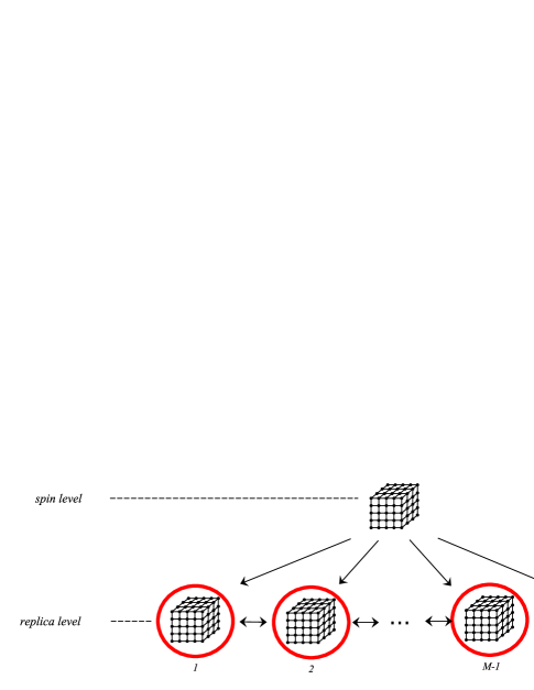
The algorithm itself is inherently data-parallel for step (4) and provides a sufficient number of data elements for a GPU implementation. In fact, there are two levels of parallelism that can be exploited; (1) spin parallelism and (2) replica level parallelism. In spin parallelism the challenge is to come up with a classic MCMC method that can take full advantage of the GPU parallel power. For this, we use a GPU-based Metropolis-Hastings implementation optimized for 3D lattices. For (2), the problem seems pleasingly parallel for a multi-GPU implementation, however special care must be put at the exchange phase, since there is a potential memory bottleneck due to the distributed memory for a multi-GPU approach. Figure 2 illustrates the two levels of parallelism and their organization.
3.2 Spin Level Parallelism
Spin parallelism corresponds to the parallel simulation of the spins of a single replica and we propose to handle it by using a single CUDA kernel based on the double checkerboard idea, proposed by M. Weigel [37, 36]. A double checkerboard approach allows the efficient simulation of spin systems using coalesced memory accesses, as well as the option to choose multiple partial sweeps in the same kernel at a much higher performance because of the GPU’s shared memory. In the original works by Weigel, the optimizations are only described and implemented for the 2D Ising Spin Glass [37, 36], but the author mentions that the ideas can be extended to 3D by using a more elaborate thread indexing scheme. The spin parallelization implementation of this work is a double 3D checkerboard and corresponds to the extension mentioned by the author.
A double checkerboard is a two-fold Metropolis-Hastings simulation strategy that is composed of several fine grained checkerboards organized into one coarse checkerboard. The case of 2D is illustrated in Figure 3.
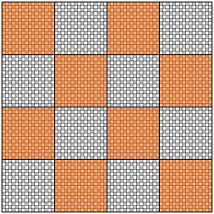
The double checkerboard method starts by simulating all spins from the orange tiles of spins, doing a local two-step black-white simulation on the fine grained checkerboard of . The tile sub-checkerboard is loaded entirely in GPU shared memory, including a halo of spins that reside on the neighbor tiles of the opposite color. After all orange tiles are finished, the same is done for the white tiles. Two kernel executions are needed to fully synchronize all threads when changing tile color. While it is true that only spins are being simulated at a given time, its advantage is that the memory access pattern is fully coalesced and the spin flip is performed in shared memory.
In order to create a double 3D checkerboard, we convert both the fine and coarse grained checkerboards to 3D. For this, we use the fact that a 3D checkerboard can be generated by using alternated 2D checkerboard layers stacked over a third dimension. For a given point in 3D discrete space, its alternation value is defined as
| (3) |
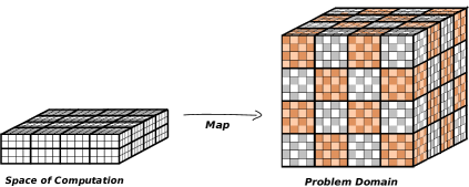
Indeed one could build a space of computation of the size of the whole lattice, launch the kernel and compute the value of using expression (3), but this approach would be inefficient because threads would remain idle waiting for its turn in the checkerboard process. Instead, we use a space of computation composed of threads; threads per block and blocks, where is the number of tiles per dimension. Figure 4 illustrates a space of computation of threads being sufficient for handling a double 3D checkerboard.
For the halos it is important to consider what percentage of the spins loaded into the GPU shared memory will actually be halo spins. Halo spins are more expensive to load into shared memory than internal tile spins due to the unaligned memory access pattern, therefore one would want the minimum number of halo spins in the shared memory. Considering that actual GPU architectures have a constant warp of threads and require a constant block volume to be specified, finding the minimum halo is equivalent to solve the optimization problem of minimizing the surface of a closed box with dimensions and constant volume . The objective function to minimize is the surface expression
| (4) |
subject to , from where we can rewrite in one variable. Setting the derivative of to zero leads to
| (5) |
where we finally get the solution: . Considering that the number of spins inside a tile is double the number of threads (because of the checkerboard approach) and that the maximum number of threads in a block is for actual GPUs, we have that . With this, and the optimal block to use is .
3.3 Replica Level Parallelism
Replica level parallelism is based on the combination of concurrent kernel execution from modern GPUs and coarse parallelism from the multi-GPU computing. In modern GPU architectures, one can launch multiple kernels in the same GPU and let the driver scheduler handle the physical resources to execute these kernels concurrently for that GPU. Starting from the Kepler GPU architecture, it is possible to launch up to kernels concurrently on a single GPU. The idea is to divide the replicas into available GPUs and simulate replicas concurrently for each GPU. It is possible that , but it is not a problem because the GPU can handle the exceeding kernels automatically with very small overhead, by using an internal execution queue. With the new approach, the new number of replicas becomes
| (6) |
where is the number of GPUs used in the multi-GPU computation. By using replicas instead of , we guarantee a balanced parallel computation for all GPUs and at the same time the extra replicas help to produce a better result. One assumes that .
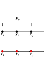
In a multi-GPU approach, the shared memory scenario transforms into a distributed scenario that must be handled using global indexing of the local memory regions. For each GPU, there is a region of memory allocated for the replicas. For any GPU , the global index for its left-most replica is while the global index for its right-most replica is .
Replica exchanges that occur in the same GPU are efficient since the swap can just be an exchange of pointers. In the limit cases at and , the task is not local to a single GPU anymore, since the exchange process would need to access replicas and , both which reside in different GPUs. Because of this special case, the pointer approach is not a robust implementation technique for a multi-GPU approach, neither explicit spin exchanges because it would require several memory transfers from one GPU to another. The solution to this problem is to swap temperatures, which is totally equivalent for the result of the simulation. One just needs to keep track of which replica has a given temperature and know their neighbors. For this we use two index arrays, and , for temperatures replica sorted and replica temperature sorted, respectively. Figure 5 illustrates the whole multi-GPU approach.
The temperature swap approach is an efficient technique for single as well as for clusters of GPU-based workstations, since for each exchange only two floating point values (i.e., ) need to be swapped. This part of the algorithm results in little overhead compared to the simulation time, thus we opted to implement it on the CPU side.
4 Adaptive Temperatures
The random field, as any other system with quenched disorder, becomes difficult to study as increases. For the selection of parameters is already a complex task, since a small change on one can lead to a bad quality simulation.
One important parameter for simulation is the selection of temperatures and the distance among them. In general, for the low-temperature regime and near the transition point , the replicas need to be placed at temperatures much closer compared to the high temperature regime in order to achieve an acceptable exchange rate. If these temperature requirements are not met, the simulation may suffer from exchange bottlenecks, preventing the information to travel from one side to other. Indeed one can decide to simulate with a dense number of temperatures for the whole range, but this strategy tends to be inefficient because the simulation does much more work than it should. Based on this facts, we propose to use an adaptive method that chooses a good distribution of temperatures based on the exchange rates needed at each region.
The idea is to start with replicas, equally distributed from to . The adaptive method performs an arbitrary number of trial simulations to measure the exchange rate between each consecutive pair of replicas. After each trial simulation, an array of exchange rates is obtained and put in a min-heap. For the intervals with lowest exchange rate (with chosen arbitrarily), new replicas are introduced using its middle value as the new temperature.
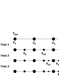
The trial simulations use multi-GPU computation. Given that the number of trial runs and the number of intervals to split is given a priori, the memory pool can be allocated before hand and equally distributed among all GPUs. After each trial run, the new -th new replica is assigned to the -th GPU with , where is the number of GPUs. The order in which new replicas are assigned to each GPU actually does not affect the performance neither the result of the simulation.
5 Performance results
In this section we present the performance results of our multi-GPU implementation (which we have named trueke for exchange in Spanish, which is trueque) and compare them against other GPU and CPU implementations. The purpose of including a comparison against a sequential CPU implementation is not to claim very high speedups, but rather to provide a simple reference point for future comparisons by the community.
5.1 Benchmark Plan
Four performance metrics, averaged over repetitions, are used to measure the parallel performance of trueke (Note, in this section means running time, not temperature):
-
1.
Benchmark the Spin-level Performance by computing the average time of a spin flip:
(7) where corresponds to the number of sweeps chosen for the Metropolis simulation.
-
2.
Benchmark the Replica-level Performance by computing the average time of a parallel tempering realization:
(8) where is the number of exchange steps chosen for the simulation.
-
3.
Benchmark the Multi-GPU Performance Scaling by measuring, based on the single GPU and multi-GPU running times , the fixed-size speedup and efficiency
(9) at different problem sizes when using two () GPUs.
-
4.
Benchmark the Adaptive Temperatures Performance by computing the average time of an adapted parallel tempering realization:
(10) where is the time for doing trials.
The number of repetitions (i.e., ) for computing the performance averages range between (i.e., less repetitions are required for benchmarking large problem sizes), which are sufficient to provide a standard error of less than .
The workstation used for all benchmarks (including the comparison implementations) is equipped with two 8-core Intel Xeon CPU E5-2640-V3 (Haswell), 128GB of RAM and two Nvidia Tesla K40 each one with 12GB.
5.2 Spin and Replica level Performance Results
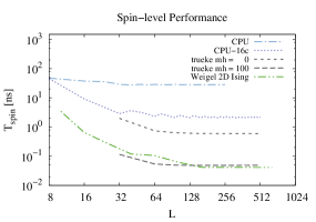
The first two benchmark results are compared, for reference, against a cache-aligned CPU implementation of the 3D Ising Random Field running both sequential and multi-core. Additionally, we include the Spin-level performance of Weigel’s GPU implementation for the 2D Ising running on our system, as a reference of how close or far trueke’s spin flip performance is compared to Weigel’s highly optimized code for 2D Ising model. The values used in Weigel’s implementation, which simulate spins, have been adapted to the form so that the input sizes can be compared against the 3D ones, in the number of total spins.
Figure 7 presents the results of spin flip time and the average parallel tempering time.
 |
 |
On the spin level performance results (left plot of Figure 7), we observe that trueke with multi-hit updates (i.e., ) is over two orders of magnitude faster than the sequential CPU implementation and over one order of magnitude faster than the multi-core CPU implementation using 16 cores. It is worth noting that trueke is almost as fast as Weigel’s highly optimized GPU Metropolis implementation for the 2D Ising model which uses too. If no multi-hit updates are used, then the performance of trueke decreases as expected, becoming faster than the multi-core implementation. It is important to consider that the comparison has been done using just one GPU for trueke while using two CPU sockets (8 cores each) for the CPU implementation. Normalizing the results to one silicon chip, one would obtain that for spin-level performance the GPU performs approximately one order of magnitude faster than a multi-core CPU. In order to obtain good quality physical results, the 3D Ising Random Field model must be simulated with . For this reason, the rest of the results do not include the case when .
The replica performance results (right plot of Figure 7) shows that the multi-GPU implementation outperforms the CPU implementation practically in the same orders of magnitude as in the spin level performance result with . This result puts in manifest the fact that the exchange phase has little impact on the replica level parallelism, indicating that multi-GPU performance should scale efficiently.
5.3 Multi-GPU Scaling
Figure 8 presents the speedup and efficiency of trueke for computing one 3D Ising Random Field simulation using two Tesla K40 GPUs.
 |
 |
From the results, we observe that as the problem gets larger, the replica level speedup improves almost to which is the perfect linear speedup. The efficiency plot shows that the replica-level parallel efficiency approaches to as the lattice becomes larger, indicating that replica-level parallelism does not degrade when increasing . This favorable behavior can be explained in part by the fact that the work of the exchange phase grows at least as where the term is the sequential work for exchanging the replicas, while the term is the parallel work for computing the energy at each replica, which is done with a parallel GPU reduction, in time for each replica. It is clear that the amount of parallel work grows faster than the sequential work, therefore the parallel efficiency of the whole method should be higher as and the number of GPUs increase.
5.4 Performance of The Adaptive Temperatures Technique
Table 1 presents the running times of the adaptive temperatures technique compared to dense and spare homogeneous techniques for . The simulation parameters used for all simulations were disorder realizations, each one with parallel tempering steps and Metropolis sweeps. For , the adaptation phase used trial runs with insertions at each trial. For , the adaptation used trial runs, with insertions at each trial. The trial runs also use parallel tempering steps with Metropolis sweeps.
| L | sparse-sim | dense-sim | adapt-trials | adapt-sim | adapt (trials + sim) |
|---|---|---|---|---|---|
| 32 | 670.25 | 1417.04 | 41.84 | 1167 | 1209.49 |
| 64 | 10386.75 | 26697.17 | 1689.46 | 19994.70 | 21684.15 |
From the results, it is observed that a full adaptive simulation, including its adaptation time, is more convenient than a dense simulation with no adaptation from the point of view of performance. The sparse technique is the fastest one because it simply uses less replicas, but as it will be shown in the next Section, it is not a useful approach for a disordered system starting from , neither the dense one, because the exchange rate becomes compromised at the low temperature regime.
6 Exchange Rates with Adaptive Temperatures
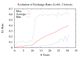
Results on the exchange rate of the adaptive strategy is presented by plotting the evolution of the average, minimum and maximum exchange rates through the trial runs. Also a comparison of the exchange rates between a dense homogeneous set, the adaptive set and a sparse homogeneous set is presented. The simulation parameters were the same as the ones used to get the performance results of Table 1. Figure 9 presents the results.
 |
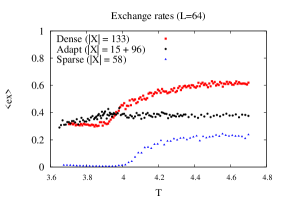 |
From the left plot we observe that as more replicas are added, the average and minimum exchange rates increase and tend to get closer, while the maximum exchange rate stabilizes after starting from trial number . For the right plot, it is clearly shown that the dense approach, although is an homogeneous approach, does not generate an homogeneous exchange rate value for the whole temperature range. For the sparse approach the scenario is even worse because at the low temperature regime there almost no exchanges. On the other hand, the adaptive method generates an exchange rate that is almost homogeneous for the entire range, which is preferred in order to have more control of the simulation. The numbers on the labels indicate the number of replicas used, and it can be seen that the adaptive method uses less replicas than the dense homogeneous approach, therefore it runs faster.
7 Preliminary Physical Results
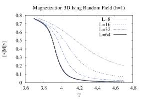
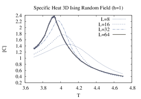
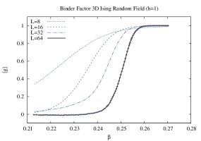
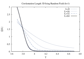
For the correctness of the whole algorithm, including the exchange phase, we ran simulations in the 3D Random Field Ising Model with field strength . The observables have been measured using parallel tempering steps, sweeps at each step, measurement at each parallel tempering step and using the adaptive temperatures technique.
Average observables are computed as , where corresponds to the average over different disorder realizations and denotes the thermal average for a single random field configuration. The magnetization is defined as
| (11) |
The specific heat is
| (12) |
where is the average energy per site. The Binder factor is an average at the disorder realization level and it is defined as:
| (13) |
and the correlation length is
| (14) |
with:
| (15) | ||||
| (16) | ||||
| (17) |
where , is the disordered magnetic field value at spin and correspond to the spatial coordinates of a given spin in the lattice. For visual clarity, we only included the error bars of the largest size studied, i.e., , nevertheless it is worth mentioning that the error bars for were even smaller than the ones for . The results are presented in Figure 10 and confirm the transition-like behavior at , or , as shown by Fytas and Malakis in their phase diagram when [11].
 |
 |
 |
 |
The results presented in this section are preliminary, with up to disorder realizations for (less for ), each doing exchange Monte Carlo steps with Metropolis-Hastings sweeps between exchanges. A physical paper devoted to the physical results will be prepared for the future.
8 Discussion
We presented a multi-GPU implementation of the Exchange Monte Carlo method, named trueke, for the simulation of the 3D Ising Random Field model. The parallelization strategy is organized in two levels; (1) spin-level parallelism, which scales in the presence of more cores per GPU, and (2) the replica-level parallelism that scales in the presence of additional GPUs. The spin-level parallelism is up to two orders of magnitude faster than its CPU counterpart when using multi-hit updates, and between one and two orders of magnitude faster when not using multi-hit updates. The parallel scaling of the method improved as the problem size got larger, in part because the amount of parallel work increases faster than the sequential work (i.e., exchange phase). This behavior is indeed favorable for multi-GPU computation, where trueke achieved approximately up to of efficiency when using two GPUs. Due to hardware limitations, we could not go beyond two GPUs, which would have been ideal for having a better picture of how the performance would scale in large systems. Nevertheless, we intend to put trueke available to the community in the near future, so that it can be benchmarked in systems with a high number of GPUs.
The adaptive strategy for selecting the temperature set was based on the idea of inserting new temperatures in between the lowest exchange rates found by an arbitrary number of trial runs. As a result, the simulation used more replicas at the locations were exchange rates were originally low, and less replicas were the exchange rate was already good, such as in the high temperature regime. The adaptive strategy outperformed any homogeneous approach, since these last ones had to deal with an over-population of replicas at places that actually did not require more temperature points, resulting in extra computational cost and slower performance, and an under-population of replicas at the low temperature regime near , generating low exchange rates. The adaptive method works better when a small number of points are added at each trial run, i.e., between one and five insertions at each trial run, because this way is more unlikely to misplace an insertion. Compared to the method by Katzgraber et. al. [18], our adaptive method differs since it feedbacks from the local exchanges of pairs of temperatures, always lifting the minimum values observed by inserting new temperatures, while in the work of Katzgraber et. al. they feedback by counting the number of times a replica travels the whole temperature range and based on this information they move the temperature set. In the method by Bittner et. al [4], they vary the number of Metropolis sweeps based on the auto-correlation times in order to avoid two replicas getting trapped exchanging together, which they identify as a problem for Katzgraber method. Our approach of inserting new temperatures provides the advantage that it does not compromise the rest of the temperature range and the technique by itself is general since it is just based on improving the lowest minimum exchange rates observed at each trial run. For the near future, we intend to do a formal comparison of all three implementations of the methods.
The main reason for choosing multi-GPU computing at the replica-level, and not at the realization level (fully independent parallelism) as one would naturally choose, is mostly because the latter strategy is not prepared for the study of large lattice systems, which would be of great interest for the near future. From our experience with the 3D RFIM, the number of replicas needed to keep at least of exchange rate grew very fast as increased. Thus, distributing the replicas dynamically across several GPUs extends the possibilities of studying larger disordered lattices.
The multi-GPU approach proposed, alias trueke, has allowed us to study th 3D Ising Random Field model at size for which its results can become physical contributions to the field. It is expected that eventually, as more GPUs are used, larger lattices could be studied.
9 Acknowledgements
The authors would like to thank Prof. M. Weigel for his valuable feedback and explanations on the subject. This research has been supported by the PhD program from CONYCIT, Chile. This work is also supported by the National Science Foundation of China (NSFC) under Grant No. 11275185 and by the Open Project Program of State Key Laboratory of Theoretical Physics, Institute of Theoretical Physics, Chinese Academy of Sciences, China (No. Y5KF191CJ1).
References
- [1] A.-K. C. Ahamed and F. Magoulès. Iterative Krylov methods for gravity problems on graphics processing unit. In Proceedings of the 12th International Symposium on Distributed Computing and Applications to Business, Engineering and Science (DCABES), Kingston, London, UK, September 2nd-4th, 2013, pages 16–20. IEEE Computer Society, 2013.
- [2] A.-K. C. Ahamed and F. Magoulès. Schwarz method with two-sided transmission conditions for the gravity equations on graphics processing unit. In Proceedings of the 12th International Symposium on Distributed Computing and Applications to Business, Engineering and Science (DCABES), Kingston, London, UK, September 2nd-4th, 2013, pages 105–109. IEEE Computer Society, 2013.
- [3] C. F. Baillie and P. D. Coddington. Comparison of cluster algorithms for two-dimensional Potts models. Phys. Rev. B, 43:10617–10621, May 1991.
- [4] E. Bittner, A. Nußbaumer, and W. Janke. Make life simple: Unleash the full power of the parallel tempering algorithm. Phys. Rev. Lett., 101:130603, Sep 2008.
- [5] B. Block, P. Virnau, and T. Preis. Multi-GPU accelerated multi-spin Monte Carlo simulations of the 2d ising model. Computer Physics Communications, 181(9):1549 – 1556, 2010.
- [6] B. A. Cipra. An introduction to the Ising model. Am. Math. Monthly, 94:937–959, December 1987.
- [7] Y. Delgado. A GPU-accelerated worm algorithm. Technical report, University of Grazz, Graz, Austria, 2011.
- [8] S. F. Edwards and P. W. Anderson. Theory of spin glasses. Journal of Physics F: Metal Physics, 5(5):965, 1975.
- [9] Y. Fang, S. Feng, K.-M. Tam, Z. Yun, J. Moreno, J. Ramanujam, and M. Jarrell. Parallel tempering simulation of the three-dimensional edwards–anderson model with compact asynchronous multispin coding on GPU. Computer Physics Communications, 185(10):2467 – 2478, 2014.
- [10] E. E. Ferrero, J. P. De Francesco, N. Wolovick, and S. A. Cannas. q-state Potts model metastability study using optimized GPU-based Monte Carlo algorithms. Computer Physics Communications, 183(8):1578–1587, 2012.
- [11] N. G. Fytas and A. Malakis. Phase diagram of the 3d bimodal random-field ising model. The European Physical Journal B, 61(1):111–120, 2008.
- [12] C. Geyer. Markov Chain Monte Carlo maximum likelihood. In Proceedings of the 23rd Symposium on the Interface, pages 156–163, 1991.
- [13] W. K. Hastings. Monte Carlo sampling methods using markov chains and their applications. Biometrika, 57(1):97–109, 1970.
- [14] K. A. Hawick, A. Leist, and D. P. Playne. Parallel graph component labelling with GPUs and CUDA. Parallel Comput., 36(12):655–678, Dec. 2010.
- [15] K. Hukushima and K. Nemoto. Exchange Monte Carlo method and application to spin glass simulations. Journal of the Physical Society of Japan, 65(6):1604–1608, 1996.
- [16] E. Ising. Beitrag zur theorie des ferromagnetismus. Zeitschrift Für Physik, 31(1):253–258, 1925.
- [17] H. G. Katzgraber, M. Körner, and A. Young. Universality in three-dimensional Ising spin glasses: A Monte Carlo study. Physical Review B, 73(22):224432, 2006.
- [18] H. G. Katzgraber, S. Trebst, D. A. Huse, and M. Troyer. Feedback-optimized parallel tempering Monte Carlo. Journal of Statistical Mechanics: Theory and Experiment, 2006(03):P03018, 2006.
- [19] Y. Komura and Y. Okabe. GPU-based single-cluster algorithm for the simulation of the ising model. J. Comput. Phys., 231(4):1209–1215, Feb. 2012.
- [20] Y. Komura and Y. Okabe. Gpu-based Swendsen-wang multi-cluster algorithm for the simulation of two-dimensional classical spin systems. Computer Physics Communications, 183(6):1155–1161, 2012.
- [21] Y. Komura and Y. Okabe. Multi-GPU-based Swendsen–Wang multi-cluster algorithm for the simulation of two-dimensional q-state Potts model. Computer Physics Communications, 184(1):40 – 44, 2013.
- [22] M. Lulli, M. Bernaschi, and G. Parisi. Highly optimized simulations on single- and multi-gpu systems of the 3d ising spin glass model. Computer Physics Communications, pages –, 2015.
- [23] F. Magoulès, A.-K. C. Ahamed, and R. Putanowicz. Auto-tuned krylov methods on cluster of graphics processing unit. International Journal of Computer Mathematics, (in press), 2014.
- [24] N. Metropolis, A. Rosenbluth, M. Rosenbluth, A. Teller, and E. Teller. Equation of state calculations by fast computing machines. J. Chem. Phys., 21:1087, 1953.
- [25] C. A. Navarro, N. Hitschfeld-Kahler, and L. Mateu. A survey on parallel computing and its applications in data-parallel problems using GPU architectures. Commun. Comput. Phys., 15:285–329, 2014.
- [26] A. T. Ogielski and I. Morgenstern. Critical behavior of three-dimensional Ising spin-glass model. Physical Review Letters, 54(9):928, 1985.
- [27] R. B. Potts. Some generalized order-disorder transformations. Cambridge Philos. Soc. Math. Proc., 48:106–109, 1952.
- [28] T. Preis, P. Virnau, W. Paul, and J. J. Schneider. GPU accelerated Monte Carlo simulation of the 2d and 3d ising model. Journal of Computational Physics, 228(12):4468 – 4477, 2009.
- [29] N. Prokof’ev and B. Svistunov. Worm Algorithms for Classical Statistical Models. Physical Review Letters, 87(16):160601+, 2001.
- [30] H. Rieger, L. Santen, U. Blasum, M. Diehl, M. Jünger, and G. Rinaldi. The critical exponents of the two-dimensional Ising spin glass revisited: exact ground-state calculations and Monte Carlo simulations. Journal of Physics A: Mathematical and General, 29(14):3939, 1996.
- [31] A. D. Sokal. Overcoming critical slowing-down: Where do we stand 23 years after Swendsen and Wang? In 104th Statistical Mechanics Conference. Rutgers University, 2010.
- [32] R. H. Swendsen and J.-S. Wang. Replica Monte Carlo simulation of spin-glasses. Phys. Rev. Lett., 57:2607–2609, Nov 1986.
- [33] R. H. Swendsen and J.-S. Wang. Nonuniversal critical dynamics in Monte Carlo simulations. Phys. Rev. Lett., 58:86–88, Jan 1987.
- [34] M. Weigel. Connected-component identification and cluster update on graphics processing units. Phys. Rev. E, 84:036709, 2011.
- [35] M. Weigel. Simulating spin models on GPU. Computer Physics Communications, 182(9):1833–1836, 2011.
- [36] M. Weigel. Performance potential for simulating spin models on GPU. Journal of Computational Physics, 231(8):3064–3082, 2012.
- [37] M. Weigel. Simulating spin models on GPU: A tour. International Journal of Modern Physics C, 23(08), 2012.
- [38] U. Wolff. Collective Monte Carlo updating for spin systems. Phys. Rev. Lett., 62:361–364, Jan 1989.