Prestructuring sparse matrices with dense rows and columns via null space methods

Abstract

Several applied problems may produce large sparse matrices with a small number of dense rows and/or columns, which can adversely affect the performance of commonly used direct solvers. By posing the problem as a saddle point system, an unconventional application of a null space method can be employed to eliminate dense rows and columns. The choice of null space basis is critical in retaining the overall sparse structure of the matrix. A one-sided application of the null space method is also presented to eliminate either dense rows or columns. These methods can be considered techniques that modify the nonzero structure of the matrix before employing a direct solver, and may result in improved direct solver performance.

1 Introduction

Modern direct solvers for large sparse linear systems usually consist of three phases: a symbolic analysis phase, a numerical factorization phase, and a solution phase, with some approaches combining aspects of symbolic and numerical factorization [19]. Much of the recent advancements in the efficiency of these solvers can be attributed in no small part to advances in algorithms used in the symbolic phase, which examines the structure of the coefficient matrix, i.e. the pattern of zero/nonzero entries. A thorough analysis of the structure lends intelligence that helps algorithms avoid numerical operations on zero entries, order rows and/or columns for a more efficient numerical factorization, reduce the amount of fill (zero entries being converted to nonzeros) in $LU$ factorizations, and results in more efficient data structures and memory allocation. Thus the structure of the coefficient matrix imparts significant influence on the efficiency in solving a large sparse linear system via direct methods.

This contrasts with iterative methods, the efficiency of which may be influenced greatly by the condition number of the coefficient matrix. To improve the potential performance of iterative methods, preconditioning techniques have been studied extensively [4]. In essence, preconditioning can be thought of as a modification of the linear system prior to solution with the intention of improving iterative solver performance.

A preconditioning analogue for direct solvers would be a technique that modifies the nonzero structure of the coefficient matrix prior to entering the symbolic analysis phase of a modern direct solver, with the intention of realizing gains in solver performance. This sort of approach can be thought of as a prestructuring technique. One potential pitfall encountered in the symbolic analysis phase of a direct solver is the presence of one or more “dense” rows in an otherwise sparse coefficient matrix. Here the definition of dense will be taken from [19]: a row of an $n\times n$ matrix is dense if it contains more than $10\sqrt{n}$ entries. The work presented here develops a prestructuring technique that may improve the performance of the direct solver by removing dense rows (as well as a dense columns) from the structure of the matrix.

The general approach to this technique will be derived from posing the linear system as a saddle point system. Several applications of numerical methods result in large, sparse systems of linear equations $M\bm{u}=\bm{b}$ where

$$M=\begin{bmatrix}A&B_{1}^{T}\\ B_{2}&C\end{bmatrix},\qquad\bm{u}=\begin{bmatrix}\bm{x}\\ \bm{y}\end{bmatrix},\qquad\bm{b}=\begin{bmatrix}\bm{f}\\ \bm{g}\end{bmatrix},$$ (1)

where $M\in^{(n+m)\times(n+m)}$ is invertible, $n\geq m$, $\displaystyle A\in^{n\times n}$, $B_{1},B_{2}\in^{m\times n}$, $C\in^{m\times m}$, $\bm{x},\bm{f}\in^{n}$, and $\bm{y},\bm{g}\in^{m}$. Matrices $M$ with the structure in (1) with $B_{1}\neq B_{2}$ are referred to as generalized saddle point matrices. Saddle point problems arise in several contexts, including computational fluid dynamics and solid mechanics, constrained optimization problems, optimal control, circuit analysis, economics, and finance. Consequently, the numerical solution of saddle point problems is a rich field of study - a comprehensive survey of methods for solving saddle point linear systems is given in [5]. In several of the aforementioned applications, $M$ and/or $A$ often have a structure that makes modern direct solvers a popular choice.

Most solution approaches for saddle point problems are designed to exploit the structure of $M$ and properties that $A,B_{1}$, and $B_{2}$ might also satisfy. Null space methods, also known as reduced Hessian or force methods, constitute one class of solution techniques for saddle point problems when $C=0$. They have arisen in several contexts, including constrained optimization [15], structural and fluid mechanics [54, 2], electrical engineering [13], and, more recently, mixed finite element approximation of Darcy and Stokes problems [3, 49, 47, 48] and continuum models for liquid crystals [58].

Of particular interest in the current context is the situation when $n$ is large, $A$ is sparse, $m$ is very small, $\text{rank}(A)\geq n-m$, and one or both of $B_{1},B_{2}$ contain dense rows. In this case $M$ may be referred to as a “bordered” system [33, 34] as the possibly-dense blocks $B_{2}$ and $B_{1}^{T}$ border the sparse matrix $A$. This situation can occur in finite element approximation of PDEs in which a constraint (such as a particular unknown having zero mean over the spatial domain) is enforced on a subset of unknowns via a global scalar Lagrange multiplier. Systems with this particular structure can also arise in numerical continuation methods for large nonlinear systems of equations which are parametrized with respect to a pseudo-arclength parameter [43, 44, 45, 46]. Other applications that can result in the presence of at least one dense row and/or column in a sparse matrix include optimization, least squares, and circuit analysis [50].

The general principle behind null space methods is to characterize the null space of the constraint (off-diagonal) operators in a saddle point system and use that characterization to reduce the saddle point system to two significantly smaller systems with nice properties of size $(n-m)\times(n-m)$ and $m\times m$. Thus, most applications of null space methods are geared towards problems where $n-m$ is small. Another particular advantage of null space methods is that the matrix $A$ need not be invertible. The main drawback of a null space method is the work required to compute null bases for the matrices $B_{1}$ and $B_{2}$. In general this can be a difficult problem [16, 17] and even more so when the matrix $Z_{k}$, whose columns form a basis for the null space of $B_{k}$, is required to have additional properties, such as sparsity or orthogonality [29, 56]. The null space method also requires $C=0$.

The objective of this paper is to consider an unconventional application of a null space method to (1) when $m$ is small and at least one of $B_{1}$ or $B_{2}$ is dense. The null space method can eliminate the dense row and column from the linear system while retaining as much of the sparse structure in $A$ as possible, thereby preserving properties of $A$ that make it attractive for direct linear solvers. With the right choice of null bases (of dimension $n-1$) the resulting system can often be solved in a fraction of the time of the original system using direct solvers. While a typical application of the null space method is designed to significantly reduce the overall size of the linear systems involved but requires significant overhead in computing the null basis, the application of a null space method described here only reduces the size of the overall system (1) by $m+1$ equations and $m+1$ unknowns and the null basis is easy to compute. Therefore, the techniques developed here can be viewed as prestructuring techniques for systems with dense rows or columns before solution with a direct solver.

The method presented here can also be applied when one of $B_{1}$ or $B_{2}$ is not dense, and can be applied to matrices with dense rows and/or columns anywhere in the matrix by first performing row or column interchanges to arrive at the structure given in (1). A “one-sided” application of the null space method to systems with $C\neq 0$ will also be developed which, when employed to remove dense rows, can increase solver performance.

It should be noted that several numerical algorithms for bordered systems arising in continuation methods and other applications have been studied [10, 8, 9, 12, 11, 32, 33, 7] and may be applied to (1) when $B_{1}$ or $B_{2}$ is dense. Several of these bordering/block-elimination/deflation methods require finding bases of the left and right null spaces of $A$, or require $C\neq 0$ in (1) and a (potentially dense) rank-1 update of $A$. Other techniques for dealing with dense rows that have arisen in the study of solving linear least squares problems include splitting algorithms [60] as well as matrix stretching [1, 35], which increases the size of the coefficient matrix to modify the sparsity pattern, thereby reducing the effect of dense rows. However, no existing methods for dealing with dense rows in sparse matrices are known to maintain or reduce the overall size of the problem and retain the overall sparsity and structural properties (such as bandedness) of the remainder of the coefficient matrix.

The rest of this paper is organized as follows. In Section 2, the mathematical background is described, and an example of how a dense row can affect certain aspects of direct solver performance are explored. In Section 3, the general null space method for reducing the system (1) is described, as well as a one-sided null space method. In Section 4, the particular approach for constructing the null space basis is given. Several numerical examples of the method applied to particular problems are presented Section 5, which demonstrate the utility of the method to varying degrees, and a brief summary is given in Section 6.

2 Background and Motivation

2.1 Notation and Definitions

Throughout this paper, matrices and matrix blocks will be represented with capital letters (including blocks that have only one row or column), and vectors will be represented as block matrices or with boldface lowercase letters. The matrix $A$ is comprised of entries $(a_{ij})$, and the $i$th row of $A$ is given by $A_{i*}$. The $j$th column of $A$ is denoted by $A_{*j}$ or $\bm{a}_{j}$. The Euclidean norm of the vector $\bm{x}$ is $\|\bm{x}\|$ and the infinity norm is denoted $\|\bm{x}\|_{\infty}$. The number of nonzero entries in a matrix or vector will be denoted by $|\cdot|$. The rest of the paper will ignore numerical cancellation, that is, the conversion of nonzero entries to zero entries via numerical operations.

For a matrix $A\in^{n\times m}$, the range (column space) of $A$ is

$$\mathcal{R}(A)=\{\bm{v}\in^{n}\,\arrowvert\,\bm{v}=A\bm{x}\text{ for some }\bm{x}\in^{m}\},$$

and the null space of $A$ is denoted by

$$\mathcal{N}(A)=\{\bm{v}\in^{m}\,\arrowvert\,A\bm{v}=0\}.$$

When the set of vectors in the range or null space come from a particular subspace $\mathcal{V}$ of ⁿ or ^m, these will be denoted by $\mathcal{R}(A|\mathcal{V})$ or $\mathcal{N}(A|\mathcal{V})$, respectively.

An $m\times n$ matrix $A$ with $m\geq n$ has the Hall property if every set of $k$ columns, $1\leq k\leq n$, contains nonzeros in at least $k$ rows, and $A$ has the strong Hall property when every set of $k$ columns, $1\leq k\leq n-1$, contains nonzeros in at least $k+1$ rows.

Graphs are defined by vertex and edge sets. Vertices will be denoted by number; $\langle i,j\rangle$ represents a directed or undirected edge between vertices $i$ and $j$, in which case vertices $i$ and $j$ are adjacent. The degree of a vertex $i$ is the number of adjacent vertices, which is also the number of edges that originate or terminate at vertex $i$. The indegree and outdegree are the number of edges leading into and out of a vertex of a directed graph, respectively.

It will be useful to describe the nonzero pattern of a matrix using a bipartite graph: for a general $m\times n$ matrix $A$, the bipartite graph $H(A)$ consists of row vertices $1^{\prime},2^{\prime},\ldots,m^{\prime}$, column vertices $1,2,\ldots,n$, and edges $\langle i^{\prime},j\rangle$ when $A_{ij}\neq 0$. In this paper the convention will be to display row vertices along a horizontal line below the horizontal line containing the column vertices. Additionally, with bipartite graphs, the direction of edges are obvious so arrows will be suppressed.

The layered graph $L(AB)$ of a matrix product $AB$ is a graph with three rows of vertices: it is the graph $H(B)$ placed on top of the graph $H(A)$ so that the column vertices of $A$ are the row vertices of $B$. The layered graph is easily generalized to represent the product $A_{1}A_{2}\cdots A_{r}$. There is a path from vertex $i$ to vertex $j$ in a directed (or undirected) graph if there is a sequence of vertices $(v_{1},v_{2},\ldots,v_{k})$ such that $v_{1}=i$, $v_{k}=j$, and $v_{\ell}$ is adjacent to $v_{\ell+1}$ for $1\leq\ell<k$.

To illustrate how the nonzero pattern of the product of sparse matrices is determined from the associated layered graph, the following result, adapted from Proposition 1 of [14], will be utilized.

Lemma 1.

Let $A\in^{m\times n}$ and $B\in^{n\times p}$. Assuming no numerical cancellation,

1. The number of nonzero entries in the $i$th row of $AB$ equals the number of $B$ column vertices in the layered graph $L(AB)$ of $AB$ that the $i$th row vertex of $A$ reaches via directed paths.

2. The number of nonzero entries in the $i$th column of $AB$ is equal to the number of $A$ row vertices in the layered graph $L(AB)$ of $AB$ that can reach the $i$th column vertex of $B$.

An example of the application of Lemma 1 is illustrated below. In (2) the nonzero entries of each of $A$ and $B$ are represented with $\times$, and Figure 1 gives the layered graph $L(AB)$. Each possible path from a row vertex of $A$ on the bottom row to a column vertex of $B$ on the top row gives a nonzero entry in $C=AB$, provided there is no numerical cancellation.

$$AB=\begin{bmatrix}&\times&&\times&\\ \times&&&\times&\times\\ &&\times&&\\ \times&\times&&&\times\\ &&&\times&\end{bmatrix}\begin{bmatrix}\times&&&&\\ &\times&&\times&\\ &\times&&&\times\\ &&\times&&\\ \times&\times&&&\end{bmatrix}=\begin{bmatrix}&\times&&\times&\\ \times&\times&\times&&\\ &\times&&&\times\\ \times&\times&&\times&\\ &&\times&&\end{bmatrix}=C.$$ (2)

Fig. 1: Illustration of the nonzero pattern of $C=AB$ in (2) using the layered graph $L(AB)$.

2.2 Dense Rows/Columns and Direct Solvers

While a complete analysis of the effect that a dense row and/or column has on all aspects of particular direct solvers is beyond the scope of this work, a brief discussion and some examples of easily observed phenomena will be presented.

During symbolic analysis, solvers typically employ directed and/or undirected graph data structures and algorithms for analyzing the nonzero pattern of a sparse matrix. This in turn is often used to allocate memory to store the $L$ and $U$ factors of the matrix, as well as determine row or column orderings that may reduce the amount of fill encountered during the numerical factorization. The reference [19] provides a broad summary of data structures and graph algorithms for direct Cholesky, QR, and LU factorization procedures. Summarizing several published theoretical results [28, 25, 27], Theorems 6.1 and 6.2 of [19] specify the following about the strong Hall matrix $A$, where $PA=LU$ (with $P$ determined by partial pivoting) and $A=QR$ (the QR factorization), assuming no numerical cancellation:

1. An upper bound for the structure of $U$ is given by the structure of $R$.

2. An upper bound for the structure of $L$ is given by the structure of $V$, the lower trapezoidal matrix of Householder vectors used in the QR factorization of $A$.

An elimination tree [59] is a data structure that is used in many aspects of direct solvers, including storage, row and column ordering, and symbolic and numeric factorization. For a matrix $M$ satisfying the strong Hall property, the column elimination tree [24, 57] of $M$ is the elimination tree of $M^{T}M$, and it can be used to predict potential intercolumn dependencies. Recent work has pointed to the row merge tree [53, 36, 37], based on the row merge matrix [26], as an alternative for structure prediction and can be employed for matrices satisfying only the Hall property. These trees and related structures are employed to develop upper bounds on the number of nonzeros in $Q,R,L$, or $U$ by various means.

However, the presence of a dense row in $M$ could lead to significant, if not catastrophic, fill during the elimination process. In fact, the presence of a full row in a matrix $M$ implies that $M^{T}M$ is completely full, which results in a column elimination tree of full height. Additionally, the row merge matrix of $M$ will also be full. Together these may lead to overestimates of column dependencies and the number of nonzeros in the $L$ and $U$ factors of $M$ and adversely affect several aspects of solver performance. Additionally, dense columns may affect algorithms that are used to determine row and column orderings that minimize fill [18, 19, 21, 22], especially when $A$ is not SPD or has some zero diagonal entries.

2.3 Example of Symbolic Analysis with a Dense Row and Column

The MATLAB computing environment, which utilizes the UMFPACK solver [18] for sparse, square, nonsymmetric matrices, provides a symbolic factorization command (symbfact(M,’col’)) that returns upper-bound estimates on the number of nonzeros in the numerical factorization of a matrix, as well as the column elimination tree. Additionally, MATLAB provides a spparms setting that can display detailed information about the sparse matrix algorithms employed when the MATLAB linear solve (\) is executed.

Assume $m=1$. Here let $M$ be a (lower-right pointing) arrowhead matrix, which for $m=1$ consists of a diagonal $A$, dense rows $B_{1}$ and $B_{2}$, and nonzero $C$. Arrowhead matrices, which satisfy the Hall property, arise in several applications [51], and one solution approach consists of transforming arrowhead matrices to tridiagonal matrices via chasing algorithms [61, 52]. Set $A=I_{n}$ in (1) and $B_{2}$ to be a random $n$-vector with entries between $0$ and $1$ (generated by the sprand() function) and $C=1$. The column $B_{1}^{T}$ is a full random $n$-vector ($|B_{1}|=n$) stored in sparse format. The sparse matrix $M$ is formed and then a symbolic factorization is computed. The objective of this example is to demonstrate how the density of $B_{2}$ affects the upper-bound estimates for $L$ and $U$ formed in the numerical factorization of $M$, as well as the height of the column elimination tree. All computations were performed using MATLAB R2014a. Table 1 presents statistics reported by symbfact() and spparms(’spumoni’,2) for $n=10^{4}$. In the table

• “symb time” represents the time required for symbfact();

• $h$ is the height of the column elimination tree;

• “$\overline{|L+U|}$” represents the symbolic upper bound on the number of nonzero entries in $L+U$;

• “$|L+U|$” is the true number of nonzero entries once the actual LU factorization in executed, and

• “solve time” is the time required to execute x=M\b, where b is a sparse random $n+1$-vector.

All timing results are obtained using MATLAB’s tic and toc functions and reported as seconds. It is observed that the symbolic factorization time, the height of the column elimination tree, and the upper bound on nonzeros in $L+U$ grows in proportion to $|B_{2}|$ and not $|M|$. As $|B_{2}|$ ranges from $0$ to $10^{4}$, the number of nonzeros in $M$ increases only by 50%, while the amount of storage allocated for LU factorization increases by a factor of 2500, potentially affecting the performance of the direct solver. In actuality, the time required for solving a linear system with coefficient matrix $M$ and the true number of nonzeros in $|L+U|$ scale more closely with $|M|$. For much larger $n$ (as will be reported in Section 5) however, this may not be the case.

$|M|$	$|B_{2}|$	symb time	$h$	$\overline{|L+U|}$	$|L+U|$	solve time
20001	0	0.0018	2	20001	20001	0.00019
20002	1	0.0017	2	20002	20002	0.00036
20011	10	0.0016	11	20056	20011	0.00034
20100	99	0.0017	100	24951	20100	0.00038
20945	944	0.0182	945	466041	20945	0.00060
22211	2210	0.1059	2211	2463156	22211	0.00091
23905	3904	0.3796	3905	7642561	23905	0.00139
25956	5955	0.9637	5956	17753991	25956	0.00189
30001	10000	2.7159	10001	50025001	30001	0.00285

Table 1: Solver statistics for $M$ with $n=10^{4}$ and increasing density of $B_{2}$.

3 Null Space Methods

Here the general null space method for (1) is outlined. Further exposition and details can be found in [5] for the case $B_{1}=B_{2}$ and $C=0$, and [38] for $B_{1}\neq B_{2}$. The first part of this section assumes $C=0$, and subsequently a variant of the null space method for $C\neq 0$ is described.

3.1 The Null Space Method for (1)

The following result (Theorem 3.1 of [38]) establishes the equivalence of certain requirements on the blocks of $M$ in (1) with the invertibility of $M$ when $C=0$.

Theorem 2.

The matrix $M=\left[\begin{smallmatrix}A&B_{1}^{T}\\ B_{2}&0\end{smallmatrix}\right]$ is invertible if and only if $B_{1}$ has full row rank,

$$\mathcal{N}(A)\cap\mathcal{N}(B_{2})=\{0\},$$ (3)

and

$$\mathcal{R}(A|\mathcal{N}(B_{2}))\cap\mathcal{R}(B_{1}^{T})=\{0\}.$$ (4)

As remarked in [38], if $B_{1}\in^{m\times n}$ has full row rank, then $\dim\mathcal{R}(B_{1}^{T})=m$, so (4) implies $\dim\mathcal{R}(A|\mathcal{N}(B_{2}))\leq n-m$, and (3) implies $\dim\mathcal{R}(A|\mathcal{N}(B_{2}))=\dim\mathcal{N}(B_{2})\geq n-m$, and thus $\dim\mathcal{N}(B_{2})=n-m$. This gives the following result.

Corollary 3.

If $M=\left[\begin{smallmatrix}A&B_{1}^{T}\\ B_{2}&0\end{smallmatrix}\right]$ is invertible, then $B_{2}$ has full row rank.

The null space method requires

1. a particular solution $\bm{x}^{*}$ of $B_{2}\bm{x}=\bm{g}$;

2. a matrix $Z_{1}\in^{n\times(n-m)}$ whose columns form a basis for $\mathcal{N}(B_{1})$;

3. a matrix $Z_{2}\in^{n\times(n-m)}$ whose columns form a basis for $\mathcal{N}(B_{2})$.

The algorithm proceeds by setting

$$\bm{x}:=Z_{2}\bm{v}+\bm{x}^{*}$$ (5)

so that

$$B_{2}\bm{x}=B_{2}(Z_{2}\bm{v}+\bm{x}^{*})=B_{2}Z_{2}\bm{v}+B_{2}\bm{x}^{*}=B_{2}\bm{x}^{*}=\bm{g},$$

as $B_{2}Z_{2}=0$. Substituting $\bm{x}$ into the first equation of (1) we have

$$AZ_{2}\bm{v}+B_{1}^{T}\bm{y}=\bm{f}-A\bm{x}^{*}.$$ (6)

Premultiply (6) with $Z_{1}^{T}$ to obtain

$$Z_{1}^{T}AZ_{2}\bm{v}+Z_{1}^{T}B_{1}^{T}\bm{y}=Z_{1}^{T}(\bm{f}-A\bm{x}^{*}),$$

which reduces to, as $B_{1}Z_{1}=0$,

$$Z_{1}^{T}AZ_{2}\bm{v}=Z_{1}^{T}(\bm{f}-A\bm{x}^{*}),$$ (7)

as $B_{1}Z_{1}=0$. This problem has a unique solution, as shown below.

Theorem 4.

Let $M=\left[\begin{smallmatrix}A&B_{1}^{T}\\ B_{2}&0\end{smallmatrix}\right]$ be invertible and let the columns of $Z_{1}$ and $Z_{2}$ span the null spaces of $B_{1}$ and $B_{2}$, respectively. Then $Z_{1}^{T}AZ_{2}$ is invertible.

Proof.

Let $\bm{v}\in^{n-m}$ and assume that $Z_{1}^{T}AZ_{2}\bm{v}=0$. Then $\bm{w}=AZ_{2}\bm{v}\in\mathcal{R}(B_{1}^{T})$ since $Z_{1}^{T}\bm{w}=0$ implies $\bm{w}$ is in the row space of $B_{1}$. Now, $B_{2}Z_{2}\bm{v}=(B_{2}Z_{2})\bm{v}=0$ implies $Z_{2}\bm{v}\in\mathcal{N}(B_{2})$, so it is also the case that $\bm{w}\in\mathcal{R}(A|\mathcal{N}(B_{2}))$. Thus $\bm{w}\in\mathcal{R}(A|\mathcal{N}(B_{2}))\cap\mathcal{R}(B_{1}^{T})$, and therefore Theorem 2 implies (4), so $\bm{w}=AZ_{2}\bm{v}=0$. This in turn implies $Z_{2}\bm{v}\in\mathcal{N}(A)$, and thus condition (3) implies $Z_{2}\bm{v}=0$. Hence $Z_{2}^{T}Z_{2}\bm{v}=0$, and since $\text{rank}(Z_{2}^{T}Z_{2})=\text{rank}(Z_{2})=\dim\mathcal{N}(B_{2})=n-m$, the invertiblity of $Z_{2}^{T}Z_{2}\in^{n-m}$ guarantees $\bm{v}=0$, completing the proof. ∎

Once $\bm{v}$ is found in (7), $\bm{x}$ is obtained via (5), and $\bm{y}$ is solved by premultiplication of (6) by $B_{1}$ to obtain the $m\times m$ system

$$B_{1}B_{1}^{T}\bm{y}=B_{1}\left(\bm{f}-A(Z_{2}\bm{v}+\hat{\bm{x}})\right),$$ (8)

which has a unique solution as $B_{1}B_{1}^{T}$ is invertible due to the fact that $B_{1}$ has full row rank. The null space method is summarized in Algorithm 5.

Algorithm 5 (Null Space Method for $M$).

1. Find $Z_{1}$ whose columns form a basis for the null space of $B_{1}$.

2. Find $Z_{2}$ whose columns form a basis for the null space of $B_{2}$.

3. Find $\bm{x}^{*}$ such that $B_{2}\bm{x}^{*}=\bm{g}$.

4. Solve $Z_{1}^{T}AZ_{2}\bm{v}=Z_{1}^{T}(\bm{f}-A\bm{x}^{*})$ for $\bm{v}$.

5. Set $\bm{x}=Z_{2}\bm{v}+\bm{x}^{*}$.

6. Solve $B_{1}B_{1}^{T}\bm{y}=B_{1}\left(\bm{f}-A(Z_{2}\bm{v}+\bm{x}^{*})\right)$ for $\bm{y}$.

It should be noted that when $\bm{g}=0$ (as is often the case in several applications), the particular solution $\hat{\bm{x}}$ found in Step 3 of Algorithm 5 can simply be the trivial solution. As remarked in the Introduction, the null space method is traditionally attractive when $n-m$ is small, as the systems in steps 4 and 6 of Algorithm 5 are both much smaller than the $(n+m)\times(n+m)$ system (1). However, when $m$ is small, this method can be very efficient at transforming the $(n+m)\times(n+m)$ system $M\bm{v}=\bm{b}$ (where at least one of $B_{1}$ and $B_{2}$ are dense) to a reduced system of size $(n-m)\times(n-m)$ that retains the sparse structure of $A$, perhaps making it more suitable for direct solvers.

3.2 A One-Sided Null Space Method For $C\neq 0$

As noted in [5], the null space method cannot be applied directly to the situation when $M$ has a nonzero $(2,2)$ block, i.e., when $C\neq 0$ in (1). However, the null space method can be applied when the system (1) is augmented with an auxiliary variable $\bm{w}$ to obtain

$$\hat{M}\hat{\bm{u}}=\begin{bmatrix}A&B_{1}^{T}&0\\ B_{2}&C&0\\ 0&0&I_{m}\end{bmatrix}\begin{bmatrix}\bm{x}\\ \bm{y}\\ \bm{w}\end{bmatrix}=\begin{bmatrix}\bm{f}\\ \bm{g}\\ 0\end{bmatrix}.$$ (9)

It is clear that the invertibility of $M$ implies the invertibility of $\hat{M}$. As opposed to eliminating both $B_{1}$ and $B_{2}$ from the system simultaneously, this can act as a “one-sided” null space method to eliminate one of $B_{1}$ or $B_{2}$ in one execution of Algorithm 5. Rewriting (9) as

$$\begin{bmatrix}A&B_{1}^{T}&0\\ 0&0&I_{m}\\ B_{2}&C&0\end{bmatrix}\begin{bmatrix}\bm{x}\\ \bm{y}\\ \bm{w}\end{bmatrix}=\begin{bmatrix}\bm{f}\\ 0\\ \bm{g}\end{bmatrix},$$ (10)

and setting

$$\hat{\bm{x}}=\begin{bmatrix}\bm{x}\\ \bm{y}\end{bmatrix},\quad\hat{\bm{f}}=\begin{bmatrix}\bm{f}\\ 0\end{bmatrix},\quad\hat{A}=\begin{bmatrix}A&B_{1}^{T}\\ 0&0\end{bmatrix},\quad\hat{B}_{1}^{T}=\begin{bmatrix}0\\ I_{m}\end{bmatrix},\quad\text{and}\quad\hat{B}_{2}=\begin{bmatrix}B_{2}&C\end{bmatrix},$$

(10) is represented by the system

$$\begin{bmatrix}\hat{A}&\hat{B}_{1}^{T}\\ \hat{B}_{2}&0\end{bmatrix}\begin{bmatrix}\hat{\bm{x}}\\ \bm{w}\end{bmatrix}=\begin{bmatrix}\hat{\bm{f}}\\ \bm{g}\end{bmatrix}.$$ (11)

Since the coefficient matrix in (11) is invertible, Theorem 4 applies and therefore the null space method can be utilized. Note that the null basis $\hat{Z}_{1}$ for $\hat{B}_{1}$ is simply

$$\hat{Z}_{1}=\begin{bmatrix}I_{n}\\ 0_{m\times n}\end{bmatrix},$$

and premultiplication of $\hat{A}$ by $\hat{Z}_{1}^{T}$ simply removes the $m$ zero rows from the bottom of $\hat{A}$. The null space matrix of $\hat{B}_{2}$ can be written as $\hat{Z}_{2}=\begin{bmatrix}Z_{2}^{T}&Z_{C}^{T}\end{bmatrix}^{T}$ where

$$B_{2}Z_{2}+CZ_{C}=0.$$ (12)

Algorithm 5 then produces a linear system $\hat{Z}_{1}^{T}\hat{A}\hat{Z}_{2}\hat{\bm{v}}=\hat{Z}_{1}^{T}(\hat{\bm{f}}-\hat{A}\hat{\bm{x}}^{*})$ that reduces to

$$\left(AZ_{2}+B_{1}^{T}Z_{C}\right)\hat{\bm{v}}=\bm{f}-A\bm{x}^{*}-B_{1}^{T}\bm{y}^{*},$$ (13)

where $\hat{\bm{x}}^{*}=\begin{bmatrix}\bm{x}^{*}&\bm{y}^{*}\end{bmatrix}^{T}$ is the particular solution to $\hat{B}_{2}\hat{\bm{x}}=\bm{g}$. with coefficient matrix $\hat{Z}_{1}^{T}\hat{A}\hat{Z}_{2}$ where $B_{2}$ and $C$ have been eliminated. Note that when $C$ is invertible, (12) implies $Z_{C}=-C^{-1}B_{2}Z_{2}$ and the coefficient matrix in (13) is just the Schur complement of $C$ in $M$ times $\hat{Z}_{2}$. When this is the case, $Z_{2}$ can be chosen such that $B_{2}Z_{2}=0$, thereby implying $Z_{C}=0$ and reducing (13) to

$$AZ_{2}\hat{\bm{v}}=\bm{f}-A\bm{x}^{*}-B_{1}^{T}\bm{y}^{*},$$ (14)

While this one-sided approach may not be practical when $m\gg 1$, when $m$ is small this can be easily be employed to eliminate a small number of dense rows or columns. Also note that there is no need to solve for $\bm{w}$. A summary of the procedure is given below:

Algorithm 6 (One-Sided Null Space Method for $M$).

1. Find $\hat{Z}_{2}=\begin{bmatrix}Z_{2}\\ Z_{C}\end{bmatrix}$ whose columns form a basis for the null space of $\begin{bmatrix}B_{2}&C\end{bmatrix}$.

2. Find $\bm{x}^{*}$ and $\bm{y}^{*}$ such that $B_{2}\bm{x}^{*}+C\bm{y}^{*}=\bm{g}$.

3. Solve $\hat{A}\hat{Z}_{2}\hat{\bm{v}}=\left(AZ_{2}+B_{1}^{T}Z_{C}\right)\hat{\bm{v}}=\bm{f}-A\bm{x}^{*}-B_{1}^{T}\bm{y}^{*}$ for $\hat{\bm{v}}$.

4. Set $\bm{x}=Z_{2}\hat{\bm{v}}+\bm{x}^{*}$, $\bm{y}=Z_{C}\hat{\bm{v}}+\bm{y}^{*}$.

Alternatively, if the objective is to eliminate the column $B_{1}^{T}$ in (9), permute the last two columns of $\hat{M}$ so that $\hat{B}_{1}=\begin{bmatrix}B_{1}&C^{T}\end{bmatrix}$.

4 The Null Space Method for Dense Rows and Columns

In this section the null space method to eliminate a dense row and/or column from $M$ in (1) will be described. Here it is assumed that $M$ is invertible and $B_{1}=B_{2}=B$. The algorithm for constructing $Z$ developed here can certainly be applied to the case $B_{1}\neq B_{2}$ for the null space method described in Algorithm 5.

4.1 Constructing $Z$ for $m=1$

To clearly illustrate the construction of the null space basis, in this section it will be assumed that $m=1$. The task is to compute a basis for the $(n-1)$-dimensional subspace of ⁿ that is the null space of the row vector $B$. For any $m$, a standard choice for $Z$ (from [5]) is to permute the columns of $B$ by multiplication of a suitable permutation matrix $P$ to obtain $BP=\begin{bmatrix}B_{b}&B_{n}\end{bmatrix}$, where $B_{b}$ is $m\times m$ and nonsingular, and then construct $Z$ as

$$Z=P\begin{bmatrix}-B_{b}^{-1}B_{n}\\ I_{n-m}\end{bmatrix}.$$ (15)

This ensures that $BZ=0$. Such a $Z$ is known as a fundamental basis [55], and it is clearly desirable for $B_{b}$ to be easy to invert or factor. As mentioned previously, this may be a difficult task for a larger $m$, however, for the case $m=1$ considered here the construction of $Z$ can be computed in $\mathcal{O}(n)$ time.

As there must be at least one nonzero entry in $B=\begin{bmatrix}b_{1}&b_{2}&\cdots&b_{n}\end{bmatrix}$, without loss of generality assume $b_{1}\neq 0$. Since the rank of $B$ is 1, $B_{b}$ in (15) can simply be set to $b_{1}$ and subsequently $-B_{b}^{-1}B_{n}$ is the $1\times(n-1)$ vector given by

$$B_{b}^{-1}B_{n}=\begin{bmatrix}b_{2}/b_{1},&b_{3}/b_{1},&b_{4}/b_{1},&\cdots,&b_{n}/b_{1}\end{bmatrix}.$$

However, this seemingly natural choice for $Z$ is not practical. While this construction is sparse (with exactly $(|B|-1)+(n-1)=n+|B|-2$ nonzero entries) it has a severe disadvantage when employing a null space method, as a dense $B$ implies the first row of $Z$ is also dense, which can have a drastic effect on the sparsity of products of the form $Z^{T}AZ$. In fact, if $|B|=n$, the product $Z^{T}I_{n}Z=Z^{T}Z$ will be completely full, as is illustrated in Figure 2. Since the outdegree of vertex $1^{\prime}$ in $Z$ is $n$, the layered graph $L(Z^{T}Z)$ contains a path from every row index of $Z^{T}$ to every column index of $Z$. Thus, the only situation in which $Z^{T}AZ$ will not be a full matrix is when there are no nonzero entries in the first column of $A$.

Fig. 2: Illustration of $Z$ and $Z^{T}Z$ in (15) when $|B|=n$.

Thus, an alternate method for constructing the null space basis $Z$ that allows $Z^{T}AZ$ to retain as much of the original sparse structure of $A$ as possible is desired. To achieve this, $Z$ should be constructed so that the outdegree of all rows of $Z$ is as small as possible. Following the general principle that each column $\bm{z}_{j}$ of $Z$ must be constructed so that $B\bm{z}_{j}=0$, an alternate approach can be derived from using only a single nonzero entry in $B$ to eliminate a subsequent nonzero entry. Again, without loss of generality, assume that $b_{1}\neq 0$, and also let $b_{m}$ represent the last nonzero entry in $B$ ($m\leq n$). The first step is to find the next nonzero entry in $B$, as it will be used with $b_{1}$ to produce a null vector. Starting with $j=1+1$, if $b_{j}=0$, then column $\bm{z}_{j}$ of $Z$ will simply be set to $\bm{e}_{j}\in^{n}$ (the elementary basis vector for index $j$), as this will imply $B\bm{z}_{j}=0$. If a nonzero $b_{j}$ is found, then the first column $\bm{z}_{1}$ of $Z$ is all zeros with the exception of a $1$ in entry 1 and $-b_{1}/b_{j}$ in entry $j$. This ensures that $B\bm{z}_{1}=0$. The algorithm resumes by setting $i$ equal to $j$ and then seeking the next nonzero entry in $B$. The above procedure is repeated until the last nonzero entry $b_{m}$ is encountered. At this point, $m-1$ linearly independent columns $\bm{z}_{k}$, $k=1,\ldots,m-1$, have been constructed, and $B\bm{z}_{k}=0$ for each $k$. It remains to add $n-m$ more linearly independent columns to $Z$. Since the $n-m$ entries $b_{m+1}=b_{m+2}=\cdots=b_{n}=0$, simply add the elementary basis vector $\bm{e}_{k}$, $m+1\leq k\leq n$ to complete the construction of $Z$. The procedure, which requires $\mathcal{O}(n)$ operations, is summarized in Algorithm 7. In the algorithm, $\varepsilon$ represents the smallest number that is to be treated as a numerical nonzero. Depending on the programming environment and sparse data structures employed, the algorithm can be executed very quickly, for example using the find() function and vectorized computations in MATLAB.

Algorithm 7 (Construct $Z$).

1:$Z\leftarrow 0_{n\times(n-1)}$

2:$i\leftarrow 1$

3:while $i<m$ do

4:     $Z_{i,i}\leftarrow 1$

5:     $j\leftarrow i+1$

6:     while $|b_{j}|<\varepsilon$ do

7:         $Z_{j,j}\leftarrow 1$

8:         $j\leftarrow j+1$

9:     end while

10:     $Z_{j,i}\leftarrow-b_{i}/b_{j}$

11:     $i\leftarrow j$

12:end while

13:for $i=m$ to $n$ do

14:     $Z_{i+1,i}\leftarrow 1$

15:end for

The result of the preceding discussion is summarized below.

Lemma 8.

For any $B\in^{1\times n}$ with at least one nonzero entry, the columns of $Z$ produced by Algorithm 7 form a basis for the $(n-1)$-dimensional null space of $B$. The number of nonzero entries in $Z$ is $|B|+n-2$.

While the $Z$ constructed by Algorithm 7 has exactly the same number of nonzero entries as the $Z$ given by (15), the important characteristic of this $Z$ is that each row and each column have at most 2 nonzero entries. An example of a $B$ and its corresponding $Z$ is given in (16), and the general form of $Z$ and $L(Z^{T}Z)$ when $|B|=n$ are given in Figure 3.

$$\footnotesize B^{T}=\begin{bmatrix}0\\ 1\\ -3\\ 0\\ -1\\ 2\\ 0\\ 0\end{bmatrix}\qquad\Longrightarrow\qquad Z=\begin{bmatrix}1&&&&&&\\ &1&&&&&\\ &\frac{1}{3}&1&&&\\ &&&1&&&\\ &&-3&&1&&\\ &&&&\frac{1}{2}&&\\ &&&&&1&\\ &&&&&&1\end{bmatrix}.$$ (16)

Fig. 3: Illustration of $Z$ and $Z^{T}Z$ given by Algorithm 7 when $|B|=n$.

Remark 9.

The maximum degree of any row or column vertex in $H(Z)$, where $Z$ is generated by Algorithm 7, is 2.

Figure 4 gives an example of how the nonzero pattern of $Z^{T}AZ$ is determined when $B$ is full. In this worst-case situation, while $Z^{T}AZ$ may have as many as 4 times as many nonzero entries as $A$, the product retains the overall sparse structure of $A$ and the dense row and column are eliminated from the system.

Fig. 4: The layered graph $L(Z^{T}AZ)$ for $Z$ constructed by Algorithm 7 when $|B|=n$ and a random $A$.

Theorem 10.

Assume $m=1$, $C=0$, and $B_{1}=B_{2}=B$ in (1). Let $Z\in^{n\times(n-1)}$ be given as in Algorithm 7. Then $Z^{T}AZ$ in Step 4 of Algorithm 5 satisfies $|Z^{T}AZ|\leq 4|A|$.

Proof.

The result is shown by bounding the number of nonzero entries in row $i$ of $Z^{T}AZ$ and then summing over the rows. Let $i\in 1,\ldots,n-1$ be a row vertex of $Z^{T}$. The construction of $Z$ guarantees that the outdegree of vertex $i$ at most 2. Assume the outdegree is 2 and let $j_{i,1},j_{i,2}$ be the column vertices of $Z^{T}$ reached by vertex $i$ in $H(Z^{T})$. These column vertices of $Z^{T}$ correspond to the row vertices $j_{i,1}$, $j_{i,2}$ of $A$, which have outdegree $|A_{j_{i,1}*}|$, $|A_{j_{i,2}*}|$ respectively. Each column vertex of row $j_{i,1}$, $j_{i,2}$ of $A$ corresponds to a row vertex of $Z$, all of which have an outdegree of at most 2. Thus, the number of possible paths originating from row vertex $i$ in the layered graph of $Z^{T}AZ$ is bounded by

$$|(Z^{T}AZ)_{i*}|\leq 2|A_{j_{i,1}*}|+2|A_{j_{i,2}*}|.$$

Using part 1 of Lemma 1 and summing over the rows of $Z^{T}$ gives the bound

$$|Z^{T}AZ|\leq\sum_{i=1}^{n-1}\left(2|A_{j_{i,1}*}|+2|A_{j_{i,2}*}|\right).$$ (17)

However, the indegree of any column vertex of $Z^{T}$ is at most 2 as well, which guarantees that the indices $j_{i,1}$ and $j_{i,2}$ appear at most twice in the right hand side of (17). Thus we have

$$|Z^{T}AZ|\leq\sum_{i=1}^{n-1}\left(2|A_{j_{i,1}*}|+2|A_{j_{i,2}*}|\right)\leq\sum_{j=1}^{n}2\cdot 2|A_{j*}|=4|A|,$$ (18)

which completes the proof. ∎

Remark 11.

The maximum inflation, i.e. $|Z^{T}AZ|/|M|$ when $|B|=n$ is $4-8n/|M|$. For example, if $A=I_{n}$, $|M|=3n$ which results in a maximum inflation of $4-8/3=4/3$.

Recalling the one-sided null space method in Section 3.2, a similar argument to Theorem 10 leads to the following result. Note that the last row of $\hat{Z}_{2}$ produced by Algorithm 7 contains only one nonzero entry.

Theorem 12.

Let $\hat{B}_{2}=\begin{bmatrix}B_{2}&C\end{bmatrix}$ in (1). Let $\hat{Z}_{2}\in^{n+1\times n}$ be given as in Algorithm 7. Then $\hat{A}\hat{Z}_{2}$ in Step 3 of Algorithm 6 satisfies $|\hat{A}\hat{Z}_{2}|\leq 2|A|+|B_{1}|$.

4.2 Conditioning vs. Sparsity

As remarked in [5], there is a trade-off between good conditioning properties of $Z$ and sparsity. While Algorithm 7 can easily be modified so that each column is normalized as it constructed, any orthogonalization process such as Gram-Schmidt on the columns of $Z$ will induce significant fill above (or below) the diagonal. While it is possible to construct an orthogonal basis for $\mathcal{N}(B)$ from the last $n-1$ columns of $Q$ in the QR factorization of $B$, in general this is impractical when $B$ is merely a single row and $n$ is large.

However, as the intent of this null space method is to prepare a matrix for a direct solver, conditioning may not necessarily be as significant of a concern as it is when an iterative solver is employed. It is still important to understand the general conditioning properties of $Z$. For the moment, assume $B$ is full, and let $\alpha_{i}=-b_{i}/b_{i+1}$ (i.e., the subdiagonal entries of $Z$). A simple upper bound estimate for the largest singular value $\sigma_{1}(Z)$ of $Z$ can be found using Corollary 2.4.4 of [31]. Writing $Z=I_{n\times(n-1)}+Z_{\alpha}$, we have

$$\sigma_{1}(Z)=\sigma_{1}(I_{n\times(n-1)}+Z_{\alpha})\leq\|I_{n\times(n-1)}\|_{2}+\sigma_{1}(Z_{\alpha})=1+\max_{1\leq i\leq n-1}\{|\alpha_{i}|\},$$

where $\|\cdot\|_{2}$ is the matrix 2-norm. This indicates that the relative sizes of successive nonzero entries in $B$ play a major role in the conditioning of $Z$, and suggests that permuting the rows/columns of $M$ to achieve a smaller maximum $|\alpha|$ would be advantageous. However, such an approach could destroy any desirable structure properties that $A$ enjoys, such as a small bandwidth.

Lower bounds for the smallest singular value $\sigma_{n-1}(Z)$ are not as easy. While several bounds exist in the current literature, the seemingly sharpest bounds to date [63, 62] require quantities raised to powers on the order of $n$, which is not feasible for large sparse problems. Of course, conditioning is a well-studied problem, therefore an efficient and reliable condition estimator such as MATLAB’s condest() applied to $Z^{T}Z$ should be utilized to gauge the potential impact of the null space method on $Z^{T}AZ$. When the condition number of $Z^{T}AZ$ is very large, gains in solver performance may still be realized by employing the one-sided null space method in Algorithm 6.

4.3 Extension to $m>1$

The following slight generalization of Theorem 6.4.1 in [31] allows for an easy extension of Algorithm 7 to the case $m>1$.

Lemma 13.

Let $B_{1}\in^{m_{1}\times n}$ and $B_{2}\in^{m_{2}\times n}$ have full row rank. Assume the columns of $Z_{1}\in^{n\times(n-m_{1})}$ span $\mathcal{N}(B_{1})$, and assume the columns of $Z_{2}\in^{(n-m_{1})\times(n-m_{1}-m_{2})}$ span $\mathcal{N}(B_{2}Z_{1})$. Then the columns of $Z_{1}Z_{2}$ form a basis for the null space of $\begin{bmatrix}B_{1}\\ B_{2}\end{bmatrix}$.

The nested construction of $Z^{n\times(n-m)}$ is given in the algorithm below where $B_{i}$ is the $i$th row of the $m\times n$ block $B$.

Algorithm 14 (Construct $Z$ for $m>1$).

1:Construct $Z_{1}$ for $B_{1}$ using Algorithm 7.

2:for $i=2$ to $m$ do

3:     Construct $Z\in^{(n-i+1)\times(n-i)}$ for $B_{i}Z_{i-1}\in^{1\times(n-i+1)}$ using Algorithm 7.

4:     $Z_{i}\leftarrow Z_{i-1}Z$

5:end for

Algorithm 14 constructs $Z$ in $m$ applications of Algorithm 7, $m-1$ matrix-vector products, and $m-1$ matrix multiplications, each of which are the product of two lower triangular matrices.

5 Applications of the Method

Here several applications of the null space method for systems with dense rows and columns are described. In these applications, the null space basis matrix $Z$ is constructed as given in Section 4.1. Numerical results that compare the performance of the null space method versus the standard direct solver are given.

All computations were performed on a Mac Pro with a 3.33 GHz 6-core processor and 32 GB of memory. All matrices arising in finite element methods were assembled using the FreeFEM++ environment [39]. All linear systems were solved using MATLAB R2014a. Compiled statistics include the number of nonzeros in $M$, $B_{2}$ (unless obvious), and $Z_{1}^{T}AZ_{2}$, as well as

• infl, the inflation, which is $|Z_{1}^{T}AZ_{2}|/|M|$;

• diff, which is $\|\bm{x}-\bm{x}_{*}\|_{\infty}/\|\bm{x}\|_{\infty}$, where $\bm{x}$ is the solution computed by the standard solution x=M\b and $\bm{x}_{*}$ is the solution computed by the null space method;

• Ztime, which is the time required to construct $Z_{1}$ and $Z_{2}$;

• NStime, which is the time required for the null space method set up and solution (includes Ztime);

• Stime, which is the time required to execute the direct solve x=M\b;

• and speedup, which is Stime/NStime.

The MATLAB tic and toc functions were used to capture all timing data.

5.1 Arrowhead Matrices and the One-Sided Null Space Method

In Section 2.3 arrowhead matrices were employed to demonstrate the impact of a dense row on direct solver heuristics. Let $m=1$, $A=I_{n}$, $B_{1}$ and $B_{2}$ be full vectors (in sparse format) with random entries between 0 and 1, and $C=1$. The right-hand side vector $\bm{b}$ is also full (in sparse format) with random values between 0 and 1. When the one-sided null space method described in Algorithm 6 using the null space basis given in Algorithm 7 is applied, the $(n+1)\times(n+1)$ arrowhead matrix is transformed into an $n\times n$ upper triangular matrix, which can be solved very efficiently. Table 3 in Appendix A gives statistics obtained for increasing $n$, while the plot on the left in Figure 5 shows the run times of both methods.

Fig. 5: Log-scale plot of running times for the one-sided null space method and the standard direct solve for arrowhead matrices for increasing $n$ with $|B_{1}|=n$ (left) and increasing $|B|/n$ with $n=250000$ (right) .

Similar to the example shown in Section 2.3, the effect on the increasing density of a row was also analyzed for both methods. Again, $A=I_{n}$ and $C=1$, however here $B_{1}=B_{2}=B$ is a sparse random vector with entries between 0 and 1 with a varying number of nonzero entries. Results for $n=250000$ are given in Table 4, and a plot of the running times for both methods vs. increasing $|B|/n$ is given on the right in 5. The standard direct solve time begins to increase sharply when around $10\%$ of the entries in $B$ are nonzero and experiences an overall increase in running time of more than two orders of magnitude over the range of $|B|$. In contrast, the one-sided null space method run times increase less than one order of magnitude over the entire range of $|B|$.

5.2 Elimination of Mean Zero Constraints in Finite Element Approximations

Variational problems arising from PDEs often require unknowns to be in specific subspaces of function spaces in order to be well-posed. A very common example of this is the condition that the mean value of the unknown over the spatial domain is zero. When the finite element method is employed to approximate solutions to these problems, conditions such as the mean zero constraint must also be imposed on the finite element subspaces used for approximating the unknowns.

Several software packages and environments are available to implement the finite element method. In many of the more recent packages, the end user merely needs to specify the computational mesh, specify which finite element spaces will be used, and provide the variational form of the problem. While software with these capabilities allows for great flexibility in a very short development time frame, it places certain limitations on the control available to the user. For example, it may be difficult to specify that an unknown is to be restricted to a subspace with a mean zero constraint, and it may be tedious or inefficient to modify the linear systems assembled by the software. Thus, it is often the case that the best way to implement a condition such as the mean zero constraint is via the use of a scalar Lagrange multiplier. In this case, it is straightforward to augment the original linear system produced by the method with an additional row and column that represent the additional degree of freedom and the constraint it represents. In many cases these augmented rows and columns are dense (if not full).

Typically $\Omega$ will represent a spatial domain with boundary $\Gamma$. Other notation used in this section includes the usual $L^{2}(\Omega)$ label for the Lebesgue space of square-integrable functions defined on a spatial domain $\Omega\subset^{d}$ ($d=2,3$) with Lipschitz continuous boundary $\Gamma$, and $H^{1}(\Omega)$ for those in $L^{2}(\Omega)$ with gradients also in $(L^{2}(\Omega))^{d}$. The space $H(\text{div},\Omega)$ represents the functions in $(L^{2}(\Omega))^{2}$ with divergence in $L^{2}(\Omega)$. A subscript of zero on a space indicates that it is the subspace of functions with zero mean. The pairing $(\cdot,\cdot)$ represents the $L^{2}$ inner product.

Three examples are presented, each demonstrating a different aspect of the behavior of the method. First, the performance of the null space method is compared to the standard solve for a problem with $|B|=n$ and two different nonzero patterns. Subsequently, a comparison of the null space method’s performance on the Stokes and Navier-Stokes problems on the same domain and mesh is given (with $|B|$ around 11% of $n$). Finally, a comparison of the null space method’s performance on a dual-mixed problem with a regular nonzero pattern is compared to similar systems with an irregular nonzero pattern (with $|B|$ around 40% of $n$). A summary of the comparisons between the null space method and the standard direct solve for largest problem of each of the different examples in given in Table 2.

Problem	Domain	$n+1$	Inflation	NStime	Stime	Speedup
Poisson	Square	303602	1.57	4.717	108.684	23.04
Poisson	Ring-like	473786	1.96	36.037	60.448	1.68
Mixed Stokes	Square	394189	1.33	81.795	1349.064	16.49
Mixed Navier-Stokes	Square	394189	1.21	136.018	1357.513	9.98
Dual-Mixed Stokes	Square	720961	1.03	105.158	2926.810	27.83
Dual-Mixed Stokes	Irregular	656314	1.03	38.662	1604.043	41.49

Table 2: Comparison of standard direct solve and null space method for largest problem of each type.

5.2.1 Poisson Problem with Pure Neumann Conditions

When the Poisson problem $-\Delta u=f$ in $\Omega$ is augmented with a pure Neumann boundary condition $\nabla u\cdot n=g$ on $\Gamma$, it is only well-posed provided the solution has mean zero over the spatial domain [6]. Employing a scalar Lagrange multiplier to enforce this, the variational problem results in the system

$$\begin{bmatrix}A&B^{T}\\ B&0\end{bmatrix}\begin{bmatrix}u\\ \lambda\end{bmatrix}=\begin{bmatrix}f\\ 0\end{bmatrix},$$

where $A$ is large and sparse with a (usually small) bandwidth, and $B\in^{1\times n}$ is dense, representing $\int_{\Omega}u\,d\Omega$. In this example, two different spatial domains $\Omega$ are used: the first is the unit square in ² and the finite element mesh is regular, while the second is a ring-like domain with a Delaunay mesh. Representatives of both meshes are given in Figure 6, and example sparsity plots for both problems are given in Figure 7. Continuous piecewise linear finite elements were employed to approximate $u$, and $|B|=n$ (completely full).

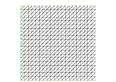
Fig. 6: Example meshes used for Poisson problem with square domain (left) and ring-like domain (right).

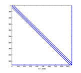
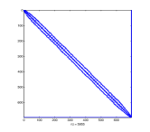
Fig. 7: Example sparsity plots for $M$ in Poisson problem with square domain (left) and ring-like domain (right).

Results of both the standard solve and null space method are presented in Table 5 in Appendix B. For problems of increasing size, using the null space method as a prestructuring technique produces a significant speedup over the original system. A visualization of the performance of both the null space method and the standard solve is given in Figure 8.

To investigate how varying nonzero patterns in $A$ may influence the performance of the null space method, the problem was also solved on a ring-like domain that consists of a circle with an elliptic section removed from the center. The null space method and the standard solve are compared in Tables 6 in Appendix B. In this case, the inflation induced by the null space method is significantly higher than the square domain, almost doubling the number of nonzero entries in $M$. For this mesh, the number of neighboring elements is generally higher than that of the square mesh, as $A$ averages around 8 nonzero entries per row for the ring-like domain, compared to an average of around 6 nonzero entries per row for the square domain. The problem on the square domain also enjoys a more uniform nonzero pattern than the ring-like domain. Overall, prestructuring the system on the ring-like domain with the null space method does not give much of an improvement over the direct solve of the original system.

Fig. 8: Log-scale plot of running times for the null space method and the standard direct solve for the pure Neumann problem on a square domain and ring-like domain.

5.2.2 Mixed Stokes and Navier-Stokes Problems

The Navier-Stokes equations model the flow of an incompressible fluid in a spatial domain. The problem with pure Dirichlet conditions is: given $f\in(L^{2}(\Omega))^{d}$, find $(u,p)$ satisfying

$$-\text{div}\left(\nu(\nabla u+\nabla u^{T})\right)+(u\cdot\nabla)u+\nabla p =f\quad \text{ in }\Omega,$$

$$\text{div}(u) =0\quad \text{ in }\Omega,$$ (19)

$$u =u_{\Gamma}\quad \text{ on }\Gamma.$$

Here $u$ is velocity, $p$ is pressure, and $\nu\geq 0$ is the kinematic viscosity. Let $L^{2}(\Omega)_{0}$ represent the functions in $L^{2}(\Omega)$ with zero average. The classical mixed finite element method for (19) poses the following variational problem: find $(u,p)\in(H^{1}(\Omega))^{d}\times L^{2}_{0}(\Omega)$ such that

$$\nu(\nabla u,\nabla v)+((u\cdot\nabla)u,v)-(p,\text{div}(v)) =(f,v)\quad \forall v\in(H^{1}(\Omega))^{d},$$ (20)

$$(\text{div}(u),q) =0\quad \forall q\in L^{2}_{0}(\Omega).$$ (21)

The Stokes problem is represented by (19) without the nonlinear $(u\cdot\nabla)u$ term. To implement the mean zero constraint on $p$ and $q$, a scalar Lagrange multiplier $\lambda$ can be introduced, and (20)–(21) is augmented by adding $\lambda\int_{\Omega}q\,d\Omega$ to the left hand side in (21) and the equation $\mu\int_{\Omega}p\,d\Omega=0$.

Table 7 gives the results of the Stokes problem using the standard Taylor-Hood finite elements for velocity and pressure on a rectangular domain [30]. This results in a dense $B$ with around $0.11n$ nonzero entries. Results obtained for the same computations for the fully nonlinear Navier-Stokes equations are displayed in Table 8. An absence of data in the “diff” and “Stime” columns indicates that the standard direct solve was not attempted. In Table 7 it is observed that the null space method can solve a system with $n+1=736030$ in less time than the standard direct solve in a system around one fourth of the size ($n+1=183076$). An example of the sparsity pattern of both $M$ and $Z^{T}AZ$ for the Navier-Stokes problem is given in Figure 9 and the comparison of times is given in Figure 10. While the null space method does not in general demonstrate as much speedup for Navier-Stokes as it does Stokes, it is important to note that several Navier-Stokes systems must be solved during an iterative nonlinear solve, so the speedup will be repeatedly realized.

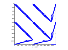
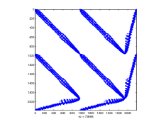
Fig. 9: Example sparsity plot of $M$ (left) and $Z^{T}AZ$ (right) for the Navier-Stokes problem.

Fig. 10: Log-scale plot of running times for the null space method and the standard direct solve for Stokes and Navier-Stokes.

5.2.3 Dual-Mixed Stokes Problems

While the velocity and pressure are the primary unknowns in the classical mixed method for the Stokes and Navier-Stokes equations, the dual-mixed method [40, 41, 42] for Stokes and Navier-Stokes approximates the fluid stress ($S$), velocity ($u$), and velocity gradient ($G$) directly. Specifically, the variational problem is: given $f\in(L^{2}(\Omega))^{d}$ and $g\in(H^{1/2}(\Gamma))^{d}$, find $(G,u,S)\in(L^{2}(\Omega))^{d\times d}\times(L^{2}(\Omega))^{d}\times\mathbb{S}$ satisfying

$$\nu(G,H)-(1/2)(u\otimes u,H)-(S,H) =0, \forall H\in(L^{2}(\Omega))^{d\times d},$$

$$(1/2)(Gu,v)-(\text{div}(S),v) =(f,v), \forall v\in(L^{2}(\Omega))^{d},$$ (22)

$$(G,T)+(u,\text{div}(T)) =\int_{\Gamma}u_{\Gamma}\cdot Tn\,d\Gamma, \forall T\in\mathbb{S},$$

where

$$\mathbb{S}=\left\{T\in(H(\text{div},\Omega))^{d\times d}\,\arrowvert\,\int_{\Omega}tr(T)\,d\Omega=0\right\}.$$

The mean trace zero constraint on $(H(\text{div},\Omega))^{d\times d}$ can be relaxed by incorporating a scalar Lagrange multiplier $\lambda\in$, yielding the linear system

$$\begin{bmatrix}A_{G}&A_{Gu}&B_{1}^{T}&0\\ A_{uG}&0&B_{2}^{T}&0\\ B_{1}&B_{2}&0&C^{T}\\ 0&0&C&0\end{bmatrix}\begin{bmatrix}G\\ u\\ S\\ \lambda\end{bmatrix}=\begin{bmatrix}0\\ F\\ g\\ 0\end{bmatrix},$$ (23)

where $C$ is the dense row that represents $\int_{\Omega}tr(S)\,d\Omega$. Linear systems for the dual-mixed Stokes problem (without the $A_{Gu}$ and $A_{uG}$ blocks in (23)) were constructed for two different spatial domains in ²: a unit square and an irregular-shaped domain. First-order Raviart-Thomas elements for $S$ and discontinuous piecewise linear elements for $G$ and $u$ were employed, resulting in $|B|\approx 0.4n$. Comparisons of the sparsity plots for the two different domains are presented in Figure 11. Results from the full null space method and the standard direct solve are given in Tables 9 and 10, and the comparisons are summarized in Figure 12. The speedup exhibited by the null space method is even greater for the irregular domain, suggesting that the removal of the dense row and column allows the algorithms in the direct solver to take a greater advantage of the lack of structure in the irregular domain problem. This can be observed by examining the supernodal column elimination tree [23] (obtained using the symbolic factorization option of the umfpack2 routine provided by SuiteSparse [20]) of both $M$ and $Z^{T}AZ$ given for $n+1=139616$ in Figure 13. Prestructuring $M$ with the null space method effectively reduces the height of the tree from 23220 to 98, vastly reducing the intercolumn dependencies.

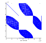
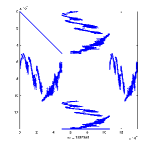
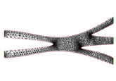
Fig. 11: Example sparsity plots of dual-mixed stokes system on square domain (left) and irregular-shaped domain (center), and irregular-shaped domain mesh (right).

Fig. 12: Log-scale plot of running times for the null space method and the standard direct solve for dual-mixed Stokes on square and irregular domains.

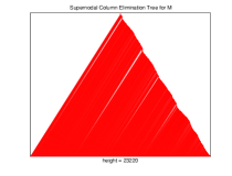
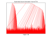
Fig. 13: Plots of supernodal column elimination tree for $M$ (left) and $Z^{T}AZ$ (right) for the dual-mixed stokes problem on irregular-shaped domain with $n+1=139616$.

6 Summary

The null space methods presented here can provide end users of direct solvers a means to avoid decreases in solver performance primarily due to the presence of dense rows. The methods are easy to implement, and the construction of the null space basis can be done in a fraction of the time required by the linear solver. Several examples demonstrate significant speedup in solving the prestructured system over the original system, however the performance of the methods appears to be limited when the inflation is significant. More investigation is required to determine under what conditions systems with the two-sided or one-sided null space method are more likely to be beneficial. While improvements in direct solver performance are continually advancing the state of the art, the techniques described here will currently allow end users of direct solvers to solve a larger class of problems with existing resources.

Appendix A Tables For Arrowhead Matrices

$n+1$	$|M|$	$|Z_{1}^{T}AZ_{2}|$	infl	diff	Ztime	NStime	Stime	speedup
25001	75001	74998	1.00	3.357E-13	0.013	0.070	0.392	5.63
50001	150001	149998	1.00	3.387E-12	0.018	0.125	1.499	11.99
75001	225001	224998	1.00	2.649E-12	0.027	0.199	3.318	16.67
100001	300001	299998	1.00	2.140E-12	0.037	0.271	5.858	21.60
125001	375001	374998	1.00	1.008E-11	0.048	0.339	9.066	26.74
150001	450001	449998	1.00	8.477E-12	0.056	0.410	12.999	31.67
175001	525001	524998	1.00	3.956E-12	0.065	0.467	17.649	37.80
200001	600001	599998	1.00	3.743E-12	0.077	0.568	23.021	40.53
225001	675001	674998	1.00	4.426E-12	0.089	0.631	29.107	46.13
250001	750001	749998	1.00	1.796E-11	0.100	0.688	35.874	52.16
275001	825001	824998	1.00	2.039E-11	0.114	0.752	43.379	57.70
300001	900001	899998	1.00	2.273E-12	0.125	0.855	51.612	60.36
325001	975001	974998	1.00	1.068E-11	0.138	0.914	60.450	66.15
350001	1050001	1049998	1.00	3.340E-11	0.151	0.999	70.263	70.34
375001	1125001	1124998	1.00	3.683E-12	0.161	1.072	80.487	75.05
400001	1200001	1199998	1.00	2.944E-11	0.173	1.138	91.617	80.54
425001	1275001	1274998	1.00	4.299E-12	0.193	1.223	103.670	84.78
450001	1350001	1349998	1.00	6.231E-11	0.199	1.276	116.110	91.03
475001	1425001	1424998	1.00	3.010E-12	0.214	1.364	129.052	94.62
500001	1500001	1499998	1.00	3.455E-11	0.224	1.427	143.563	100.57

Table 3: Comparison of standard direct solve and one-sided null space method for arrowhead matrices for increasing $n$ and $|B_{1}|=n$.

$|M|$	$|B|$	$|Z^{T}AZ|$	infl	diff	Ztime	NStime	Stime	speedup
250007	4	250004	1.00	2.79E-16	0.0085	0.104	0.269	2.60
250051	26	250048	1.00	1.44E-15	0.0079	0.111	0.292	2.63
250501	251	250498	1.00	1.04E-13	0.0079	0.107	0.278	2.59
254979	2490	254976	1.00	7.64E-13	0.0080	0.114	0.297	2.61
262349	6175	262346	1.00	7.35E-12	0.0101	0.122	0.344	2.82
274437	12219	274434	1.00	1.68E-12	0.0120	0.139	0.478	3.45
297581	23791	297578	1.00	4.27E-10	0.0245	0.165	0.965	5.86
340627	45314	340624	1.00	6.71E-11	0.0330	0.219	2.312	10.58
414717	82359	414714	1.00	2.29E-10	0.0449	0.284	5.621	19.82
446653	98327	446650	1.00	5.93E-11	0.0508	0.353	7.558	21.44
475367	112684	475364	1.00	2.16E-10	0.0567	0.373	9.339	25.05
501603	125802	501600	1.00	1.20E-09	0.0593	0.440	11.422	25.97
525071	137536	525068	1.00	5.00E-10	0.0649	0.448	13.299	29.70
566043	158022	566040	1.00	2.95E-09	0.0725	0.524	16.871	32.17
750001	250001	749998	1.00	8.54E-10	0.1028	0.722	38.479	53.32

Table 4: Comparison of standard direct solve and one-sided null space method for arrowhead matrices, $n=250000$ and increasing $|B|$.

Appendix B Tables for Poisson Problem

$n+1$	$|M|$	$|Z^{T}AZ|$	infl	diff	Ztime	NStime	Stime	speedup
40402	282003	442788	1.57	1.88E-12	0.025	0.506	2.097	4.14
51077	356628	560013	1.57	7.02E-12	0.022	0.715	3.048	4.26
63002	440003	690988	1.57	7.39E-12	0.035	0.711	5.347	7.52
76177	532128	835713	1.57	8.49E-12	0.032	1.088	6.551	6.02
90602	633003	994188	1.57	9.03E-11	0.038	1.275	9.513	7.46
106277	742628	1166413	1.57	7.63E-11	0.050	1.295	14.402	11.12
123202	861003	1352388	1.57	2.00E-10	0.060	1.804	19.159	10.62
141377	988128	1552113	1.57	3.11E-10	0.071	2.223	24.801	11.16
160802	1124003	1765588	1.57	4.59E-10	0.081	2.448	29.365	12.00
181477	1268628	1992813	1.57	5.90E-10	0.084	3.155	37.912	12.02
203402	1422003	2233788	1.57	3.61E-10	0.096	3.538	47.218	13.35
226577	1584128	2488513	1.57	2.85E-10	0.104	4.138	59.386	14.35
251002	1755003	2756988	1.57	6.12E-10	0.119	4.055	88.812	21.90
276677	1934628	3039213	1.57	5.25E-09	0.131	4.351	99.339	22.83
303602	2123003	3335188	1.57	3.92E-09	0.139	4.717	108.684	23.04

Table 5: Comparison of standard direct solve and null space method for pure Neumann problem on square domain.

$n+1$	$|M|$	$|Z^{T}AZ|$	infl	diff	Ztime	NStime	Stime	speedup
99384	890697	1704464	1.91	1.13E-09	0.035	2.282	3.514	1.54
114923	1030248	1964071	1.91	3.90E-09	0.040	2.523	4.476	1.77
132370	1186971	2368424	2.00	1.46E-09	0.048	4.978	5.797	1.16
153152	1373709	2771042	2.02	3.49E-09	0.055	6.977	7.604	1.09
175003	1570068	3003661	1.91	8.42E-09	0.064	4.266	9.805	2.30
199825	1793166	3446905	1.92	1.60E-09	0.073	5.255	12.430	2.37
217959	1956072	3753307	1.92	2.18E-08	0.081	5.826	14.788	2.54
259022	2325325	4482611	1.93	2.79E-08	0.098	13.900	19.218	1.38
263442	2364819	4756114	2.01	3.78E-08	0.104	16.351	21.262	1.30
292019	2621712	5146773	1.96	1.17E-08	0.108	16.301	25.134	1.54
327209	2938122	5844671	1.99	7.83E-10	0.124	21.092	31.279	1.48
350997	3151912	6041955	1.92	3.96E-08	0.138	10.586	35.733	3.38
387725	3482160	6644983	1.91	5.75E-08	0.152	12.487	42.870	3.43
408972	3673087	7302360	1.99	7.88E-09	0.164	31.150	47.195	1.52
473786	4256110	8353485	1.96	1.24E-08	0.194	36.037	60.448	1.68

Table 6: Comparison of standard direct solve and null space method for pure Neumann problem on ring-like domain.

Appendix C Tables for Mixed Stokes and Navier-Stokes

$n+1$	$|M|$	$|B|$	$|Z^{T}AZ|$	infl	diff	Ztime	NStime	Stime	speedup
2188	38576	257	50992	1.32	3.72E-15	0.0003	0.033	0.040	1.20
4729	84820	546	112226	1.32	4.14E-15	0.0004	0.084	0.084	1.00
8305	149502	950	198222	1.33	4.97E-15	0.0005	0.229	0.333	1.46
12772	231004	1453	305296	1.32	9.84E-15	0.0008	0.369	1.474	3.99
18517	337682	2098	447860	1.33	1.56E-14	0.0016	0.652	2.802	4.30
26854	489294	3031	646072	1.32	1.38E-14	0.0018	0.996	6.770	6.79
32995	602306	3720	796240	1.32	2.67E-14	0.0023	1.235	9.262	7.50
43078	786882	4847	1036976	1.32	4.76E-14	0.0032	1.866	15.819	8.48
51460	941098	5785	1246734	1.32	1.82E-14	0.0040	2.551	26.073	10.22
62722	1150150	7043	1523614	1.32	1.77E-14	0.0039	3.498	42.820	12.24
73372	1346148	8233	1795402	1.33	2.36E-14	0.0050	4.545	41.384	9.11
86866	1593288	9739	2121702	1.33	3.34E-14	0.0052	6.509	77.948	11.98
99460	1825198	11145	2431356	1.33	2.86E-14	0.0058	6.811	74.425	10.93
117391	2151318	13144	2859160	1.33	2.97E-14	0.0066	9.315	127.044	13.64
132352	2429104	14813	3233876	1.33	3.00E-14	0.0076	11.119	116.803	10.51
145864	2668852	16321	3543900	1.33	4.65E-14	0.0103	12.530	193.427	15.44
183076	3362662	20469	4473160	1.33	5.89E-14	0.0126	17.807	375.890	21.11
207226	3807856	23159	5056400	1.33	3.51E-14	0.0141	22.549	411.158	18.23
221359	4080710	24736	5423956	1.33	4.35E-14	0.0154	25.953	360.559	13.89
243286	4476336	27179	5959142	1.33	4.98E-14	0.0173	64.222	377.703	5.88
322522	5937362	36003	7907618	1.33	6.25E-14	0.0238	62.839	1206.523	19.20
358489	6593518	40006	8741244	1.33	5.94E-14	0.0259	132.936	1296.813017	9.76
374179	6886288	41756	9182944	1.33	8.30E-14	0.0280	74.996	1292.916187	17.24
394189	7267594	43986	9675046	1.33	7.21E-14	0.0284	72.277	1226.410117	16.97
466663	8584006	52052	11442590	1.33		0.0384	118.439
527122	9703388	58783	12932988	1.33		0.0636	136.858
590380	10854476	65825	14401620	1.33		0.0729	144.462
649570	11977796	72415	15900372	1.33		0.0787	211.806
736030	13549470	82035	18021144	1.33		0.0936	279.488

Table 7: Comparison of standard direct solve and null space method for Stokes problem.

$n+1$	$|M|$	$|B|$	$|Z^{T}AZ|$	infl	diff	Ztime	NStime	Stime	speedup
2188	60270	257	72686	1.21	1.77E-15	0.0003	0.039	0.027	0.70
4729	132406	546	159812	1.21	5.06E-15	0.0004	0.092	0.104	1.13
8305	233862	950	282582	1.21	8.31E-15	0.0005	0.201	0.244	1.21
12772	361190	1453	435482	1.21	1.01E-14	0.0007	0.312	0.703	2.25
18517	526936	2098	637114	1.21	2.10E-14	0.0013	0.560	1.151	2.05
26854	765634	3031	922412	1.20	1.28E-14	0.0023	0.952	2.327	2.44
32995	941480	3720	1135414	1.21	6.35E-12	0.0017	1.126	9.156	8.13
43078	1231012	4847	1481106	1.20	1.73E-14	0.0026	1.679	8.072	4.81
51460	1471656	5785	1777292	1.21	1.74E-14	0.0034	2.476	13.421	5.42
62722	1797106	7043	2170570	1.21	1.84E-14	0.0038	2.863	18.841	6.58
73372	2103260	8233	2552514	1.21	3.64E-12	0.0046	4.036	27.165	6.73
86866	2490402	9739	3018816	1.21	3.07E-14	0.0054	5.286	63.046	11.93
99460	2852024	11145	3458182	1.21	2.03E-10	0.0063	11.722	64.718	5.52
117391	3366344	13144	4074186	1.21	1.57E-11	0.0071	8.681	109.731	12.64
132352	3798722	14813	4603494	1.21	8.35E-12	0.0080	10.859	145.626	13.41
145864	4177670	16321	5052718	1.21	3.55E-14	0.0098	12.294	144.746	11.77
183076	5255710	20469	6366208	1.21	4.28E-14	0.0123	38.428	206.909	5.38
207226	5956162	23159	7204706	1.21	7.68E-11	0.0140	21.910	1089.682	49.73
221359	6370840	24736	7714086	1.21	4.76E-14	0.0148	47.819	310.419	6.49
243286	6994304	27179	8477110	1.21	1.97E-12	0.0159	30.516	530.607	17.39
322522	9280664	36003	11250920	1.21	5.57E-14	0.0223	124.250	2475.251	19.92
358489	10323538	40006	12471264	1.21	6.25E-14	0.0253	126.839	958.905	7.56
394189	11350622	43986	13758074	1.21	6.91E-14	0.0275	136.018	1357.513	9.98
466663	13424512	52052	16283096	1.21		0.0343	268.038
527122	15174044	58783	18403644	1.21		0.0629	147.946
590380	16981372	65825	20528516	1.21		0.0439	324.469
649570	18703960	72415	22626536	1.21		0.0493	448.260

Table 8: Comparison of standard direct solve and null space method for Naiver-Stokes.

Appendix D Tables for Dual-Mixed Stokes

$n+1$	$|M|$	$|B|$	$|Z^{T}AZ|$	infl	diff	Ztime	NStime	Stime	speedup
5081	66946	2045	68764	1.03	1.48E-14	0.0017	0.108	0.124	1.15
20161	267284	8078	274932	1.03	1.72E-14	0.0092	0.430	1.542	3.58
45241	601830	18067	619310	1.03	3.05E-14	0.0098	1.186	8.180	6.90
80321	1069456	32022	1101006	1.03	8.01E-14	0.0169	2.676	29.369	10.98
125401	1671120	49850	1720576	1.03	1.17E-13	0.0203	5.600	60.643	10.83
180481	2403874	70517	2476998	1.03	1.24E-13	0.0302	10.759	134.263	12.48
245561	3274472	97532	3371716	1.03	2.84E-13	0.0452	16.867	213.088	12.63
320641	4278110	126891	4406728	1.03	4.89E-13	0.0593	25.349	488.083	19.25
405721	5410736	161950	5570722	1.03	2.45E-13	0.0846	44.851	818.019	18.24
500801	6691372	199948	6890864	1.03	5.73E-13	0.1006	55.618	1138.317	20.47
605881	8088772	242266	8326976	1.03	3.75E-13	0.1305	83.160	1657.527	19.93
720961	9622302	284017	9913640	1.03	7.89E-13	0.1520	105.158	2926.810	27.83

Table 9: Comparison of standard direct solve and null space method for dual-mixed Stokes on a square domain.

$n+1$	$|M|$	$|B|$	$|Z^{T}AZ|$	infl	diff	Ztime	NStime	Stime	speedup
11359	148566	4668	152454	1.03	4.01E-13	0.0021	0.156	0.299	1.91
26265	346440	10680	356004	1.03	1.95E-12	0.0057	0.517	2.141	4.14
46421	614610	18767	631998	1.03	7.36E-12	0.0101	0.854	6.046	7.08
72727	965192	29323	992846	1.03	1.80E-11	0.0129	1.402	14.981	10.68
106360	1413945	42803	1454811	1.03	2.17E-11	0.0189	2.617	42.199	16.12
139616	1857691	56146	1911593	1.03	5.05E-11	0.0234	3.889	66.351	17.06
186072	2478247	74740	2550511	1.03	6.20E-11	0.0334	6.124	143.892	23.50
234428	3124189	94049	3215679	1.03	8.54E-11	0.0458	8.915	248.958	27.93
288984	3853383	115940	3966367	1.03	1.34E-10	0.0528	10.886	303.924	27.92
359490	4796221	144148	4937215	1.03	3.78E-10	0.0694	15.655	430.508	27.50
411446	5490449	164916	5652063	1.03	3.41E-10	0.0844	24.274	635.733	26.19
490102	6542539	196409	6735371	1.03	4.32E-10	0.0979	24.919	1099.457	44.12
567858	7582451	227499	7806219	1.03	4.86E-10	0.1194	27.873	1281.732	45.99
656314	8765865	262910	9024771	1.03	5.87E-10	0.1399	38.662	1604.043	41.49

Table 10: Comparison of standard direct solve and null space method for dual-mixed Stokes on an irregular domain.

References

- [1] M. Adlers and A. Björck, Matrix stretching for sparse least squares problems, Numerical Linear Algebra with Applications, 7 (2000), pp. 51–65.
- [2] M. Arioli and G. Manzini, Null space algorithm and spanning trees in solving darcy’s equation, BIT Numerical Mathematics, 43 (2003), pp. 839–848.
- [3] M. Arioli, J. Maryška, M. Rozložník, and M. Tuma, Dual variable methods for mixed-hybrid finite element approximation of the potential fluid flow problem in porous media, Electron. Trans. Numer. Anal., 22 (2006), pp. 17–40.
- [4] M. Benzi, Preconditioning techniques for large linear systems: A survey, J. Comput. Phys., 182 (2002), pp. 418–477.
- [5] M. Benzi, G. H. Golub, and J. Liesen, Numerical solution of saddle point problems, Acta Numer., 14 (2005), pp. 1–137.
- [6] S. C. Brenner and L. R. Scott, The mathematical theory of finite element methods, vol. 15 of Texts in Applied Mathematics, Springer-Verlag, New York, second ed., 2002.
- [7] D. Calvetti and L. Reichel, Iterative methods for large continuation problems, Journal of Computational and Applied Mathematics, 123 (2000), pp. 217–240. Numerical Analysis 2000. Vol. III: Linear Algebra.
- [8] T. F. Chan, Deflated decomposition of solutions of nearly singular systems, SIAM J. Numer. Anal., 21 (1984), pp. 738–754.
- [9] , Deflation techniques and block-elimination algorithms for solving bordered singular systems, SIAM J. Sci. Statist. Comput., 5 (1984), pp. 121–134.
- [10] , Techniques for large sparse systems arising from continuation methods, in Numerical methods for bifurcation problems (Dortmund, 1983), vol. 70 of Internat. Schriftenreihe Numer. Math., Birkhäuser, Basel, 1984, pp. 116–128.
- [11] T. F. Chan and D. C. Resasco, Generalized deflated block-elimination, SIAM J. Numer. Anal., 23 (1986), pp. 913–924.
- [12] T. F. Chan and Y. Saad, Iterative methods for solving bordered systems with applications to continuation methods, SIAM J. Sci. Statist. Comput., 6 (1985), pp. 438–451.
- [13] L. O. Chua, C. A. Desoer, and E. S. Kuh, Linear and Nonlinear Circuits, McGraw-Hill Book Company, 1987.
- [14] E. Cohen, Structure prediction and computation of sparse matrix products, Journal of Combinatorial Optimization, 2 (1998), pp. 307–332.
- [15] T. F. Coleman, Large Sparse Numerical Optimization, Springer-Verlag New York, Inc., New York, NY, USA, 1984.
- [16] T. F. Coleman and A. Pothen, The null space problem. I. Complexity, SIAM J. Algebraic Discrete Methods, 7 (1986), pp. 527–537.
- [17] , The null space problem. II. Algorithms, SIAM J. Algebraic Discrete Methods, 8 (1987), pp. 544–563.
- [18] T. A. Davis, Algorithm 832: Umfpack v4.3—an unsymmetric-pattern multifrontal method, ACM Trans. Math. Softw., 30 (2004), pp. 196–199.
- [19] , Direct methods for sparse linear systems, vol. 2 of Fundamentals of Algorithms, Society for Industrial and Applied Mathematics (SIAM), Philadelphia, PA, 2006.
- [20] , Algorithm 915, suitesparseqr: Multifrontal multithreaded rank-revealing sparse qr factorization, ACM Trans. Math. Softw., 38 (2011), pp. 8:1–8:22.
- [21] T. A. Davis and I. S. Duff, An unsymmetric-pattern multifrontal method for sparse lu factorization, SIAM Journal on Matrix Analysis and Applications, 18 (1997), pp. 140–158.
- [22] T. A. Davis, J. R. Gilbert, S. I. Larimore, and E. G. Ng, A column approximate minimum degree ordering algorithm, ACM Trans. Math. Softw., 30 (2004), pp. 353–376.
- [23] J. W. Demmel, S. C. Eisenstat, J. R. Gilbert, X. S. Li, and J. W. H. Liu, A supernodal approach to sparse partial pivoting, SIAM J. Matrix Anal. Appl., 20 (1999), pp. 720–755.
- [24] S. Eisenstat and J. W. H. Liu, The theory of elimination trees for sparse unsymmetric matrices, SIAM J. Matrix Anal. Appl., 26 (2005), pp. 686–705 (electronic).
- [25] A. George and E. Ng, An implementation of Gaussian elimination with partial pivoting for sparse systems, SIAM J. Sci. Statist. Comput., 6 (1985), pp. 390–409.
- [26] , Symbolic factorization for sparse Gaussian elimination with partial pivoting, SIAM J. Sci. Statist. Comput., 8 (1987), pp. 877–898.
- [27] J. Gilbert and E. Ng, Predicting structure in nonsymmetric sparse matrix factorizations, in Graph Theory and Sparse Matrix Computation, A. George, J. Gilbert, and J. Liu, eds., vol. 56 of The IMA Volumes in Mathematics and its Applications, Springer New York, 1993, pp. 107–139.
- [28] J. R. Gilbert, Predicting structure in sparse matrix computations, SIAM J. Matrix Anal. Appl, 15 (1994), pp. 62–79.
- [29] J. R. Gilbert and M. T. Heath, Computing a sparse basis for the null space, SIAM J. Algebraic Discrete Methods, 8 (1987), pp. 446–459.
- [30] V. Girault and P. Raviart, Finite Element Methods for Navier-Stokes Equations, Springer, Berlin, 1986.
- [31] G. H. Golub and C. F. Van Loan, Matrix computations, Johns Hopkins Studies in the Mathematical Sciences, Johns Hopkins University Press, Baltimore, MD, fourth ed., 2013.
- [32] W. Govaerts, Stable solvers and block elimination for bordered systems, SIAM J. Matrix Anal. Appl., 12 (1991), pp. 469–483.
- [33] W. Govaerts, Solution of bordered singular systems in numerical continuation and bifurcation, Journal of Computational and Applied Mathematics, 50 (1994), pp. 339–347.
- [34] W. J. F. Govaerts, Numerical methods for bifurcations of dynamical equilibria, Society for Industrial and Applied Mathematics (SIAM), Philadelphia, PA, 2000.
- [35] J. F. Grcar, Matrix Stretching for Linear Equations, ArXiv e-prints, (2012).
- [36] L. Grigori, M. Cosnard, and E. Ng, On the row merge tree for sparse lu factorization with partial pivoting, BIT Numerical Mathematics, 47 (2007), pp. 45–76.
- [37] L. Grigori, J. R. Gilbert, and M. Cosnard, Symbolic and exact structure prediction for sparse gaussian elimination with partial pivoting, SIAM Journal on Matrix Analysis and Applications, 30 (2009), pp. 1520–1545.
- [38] J. Haslinger, T. Kozubek, R. Kučera, and G. Peichl, Projected Schur complement method for solving non-symmetric systems arising from a smooth fictitious domain approach, Numer. Linear Algebra Appl., 14 (2007), pp. 713–739.
- [39] F. Hecht, New development in freefem++, J. Numer. Math., 20 (2012), pp. 251–265.
- [40] J. S. Howell, Approximation of generalized Stokes problems using dual-mixed finite elements without enrichment, Int. J. Numer. Meth. Fluids, 67 (2011), pp. 247–268.
- [41] J. S. Howell and N. J. Walkington, Inf-sup conditions for twofold saddle point problems, Numer. Math., 118 (2011), pp. 663–693.
- [42] , Dual-mixed finite element methods for the Navier-Stokes equations, ESAIM: Mathematical Modelling and Numerical Analysis, 47 (2013), p. 789–805.
- [43] H. B. Keller, Numerical solution of bifurcation and nonlinear eigenvalue problems, in Applications of Bifurcation Theory, P. Rabinowitz, ed., Academic Press, New York, 1977, pp. 359–384.
- [44] , Global homotopies and Newton methods, in Recent Advances in Numerical Analysis, C. de Boor and G. H. Golub, eds., Academic Press, New York, 1978, pp. 73–94.
- [45] , Practical procedures in path following near limit points, in Computing Methods in Applied Sciences and Engineering, R. Glowinski and J. L. Lions, eds., Amsterdam, 1982, Norh Holland.
- [46] H. B. Keller, The bordering algorithm and path following near singular points of higher nullity, SIAM J. Sci. Statist. Comput., 4 (1983), pp. 573–582.
- [47] S. Le Borne, Block computation and representation of a sparse nullspace basis of a rectangular matrix, Linear Algebra and its Applications, 428 (2008), pp. 2455–2467.
- [48] , Preconditioned nullspace method for the two-dimensional oseen problem, SIAM J. Scientific Computing, 31 (2009), pp. 2494–2509.
- [49] S. Le Borne and R. Kriemann, The nullspace method for the three-dimensional stokes problem, PAMM, 7 (2007), pp. 1101101–1101102.
- [50] F. Najm, Circuit Simulation, Wiley, 2010.
- [51] D. P. O’Leary and G. W. Stewart, Computing the eigenvalues and eigenvectors of symmetric arrowhead matrices, J. Comput. Phys., 90 (1990), pp. 497–505.
- [52] S. Oliveira, A new parallel chasing algorithm for transforming arrowhead matrices to tridiagonal form, Math. Comp., 67 (1998), pp. 221–235.
- [53] , Exact prediction of QR fill-in by row-merge trees, SIAM J. Sci. Comput., 22 (2000), pp. 1962–1973 (electronic).
- [54] R. J. Plemmons and R. E. White, Substructuring methods for computing the nullspace of equilibrium matrices, SIAM Journal on Matrix Analysis and Applications, 11 (1990), pp. 1–22.
- [55] A. Pothen, Sparse Null Bases and Marriage Theorems, PhD thesis, Cornell University, Ithaca, New York, 1984.
- [56] A. Pothen, Sparse null basis computations in structural optimization, Numer. Math., 55 (1989), pp. 501–519.
- [57] A. Pothen and S. Toledo, Elimination Structures in Scientific Computing, Chapman and Hall/CRC, 2015/07/01 2004, pp. 59–1–59–29.
- [58] A. Ramage and J. Eugene C. Gartland, A preconditioned nullspace method for liquid crystal director modeling, SIAM Journal on Scientific Computing, 35 (2013), pp. B226–B247.
- [59] R. Schreiber, A new implementation of sparse Gaussian elimination, ACM Trans. Math. Software, 8 (1982), pp. 256–276.
- [60] C. Sun, Dealing with dense rows in the solution of sparse linear least squares problems, tech. report, Cornell University, 1995.
- [61] H. Y. Zha, A two-way chasing scheme for reducing a symmetric arrowhead matrix to tridiagonal form, J. Numer. Linear Algebra Appl., 1 (1992), pp. 49–57.
- [62] L. Zou, A lower bound for the smallest singular value, J. Math. Inequal., 6 (2012), pp. 625–629.
- [63] L. Zou and Y. Jiang, Estimation of the eigenvalues and the smallest singular value of matrices, Linear Algebra Appl., 433 (2010), pp. 1203–1211.