Scaling functions of two-neutron separation energies of ${}^{20}C$ with finite range potentials

Abstract

The behaviour of an Efimov excited state is studied within a three-body Faddeev formalism for a general neutron-neutron-core system, where neutron-core is bound and neutron-neutron is unbound, by considering zero-ranged as well as finite-ranged two-body interactions. For the finite-ranged interactions we have considered a one-term separable Yamaguchi potential. The main objective is to study range corrections in a scaling approach, with focus in the exotic carbon halo nucleus ${}^{20}C$.

1 Introduction and Model

In the present contribution our aim is to consider a general scaling model for three-body system with two non-identical ones near the unitary limit (when one or both two-body scattering lengths have absolute values very large), by considering bound neutron-core (nc) subsystem. The approach is exemplified for the exotic carbon halo nucleus ${}^{20}C$, where an Efimov Efimov excited energy state is studied within a three-body Faddeev formalism for $n-n-^{18}C$ (also named neutron-neutron-core, $nnc$, for more general neutron-rich exotic nuclei). More details on related studies, one can obtain from AmorimPRC97 ; Marcelo ; Hammer ; Tobias ; Phillips1 ; Phillips2 and references therein. Therefore, the first task was to solve the coupled $s-$wave Faddeev integral equation using a zero-range potential to obtain the two-neutron ($nn$) separation energies for the ground and excited states of ${}^{20}C$. Next, by fixing the energy of the virtual state of the $nn$ subsystem to $E_{nn}=-143$ keV, we vary a three-body parameter in order to obtain different ${}^{19}C$ binding energies for the $n-^{18}C$ subsystem, such that we can also reproduce the ${}^{20}C$ ground-state energy, namely $E^{(0)}_{{}^{20}C}$. This procedure is followed by the calculation of the first excited-state energy $E^{(1)}_{{}^{20}C}$. In this way, we are able to obtain a scaling plot, which is conveniently given in dimensionless quantities, as $\displaystyle\sqrt{\left[{E^{(1)}_{{}^{20}C}-E_{{}^{19}C}}\right]/{E^{(0)}_{{}^{20}C}}}$ versus $\displaystyle\sqrt{{E_{{}^{19}C}}/{E^{(0)}_{{}^{20}C}}}$ Tobias ; scale . In order to study the range corrections, the same above steps are repeated, with the zero-range interaction being replaced by a separable Yamaguchi potentialYamaguchi , with an appropriate range parameter $\beta$.

In the following we present the corresponding model-formalism, where for the two-body interactions we have used zero-ranged potentials (constant in momentum space), renormalized to give us the corresponding energies of the two-body subsystems ($nn$ and $nc$), as well as finite-range interactions, given by one-term separable Yamaguchi form-factors. In the case of the finite-ranged interactions, the two-body potential, with strength $\lambda$ and range-parameter $\beta$, is given by

$$v(p,p^{\prime})=\lambda\,g(p)\,g(p^{\prime})=\lambda\,\left(\dfrac{1}{p^{2}+\beta^{2}}\right)\left(\dfrac{1}{p^{\prime 2}+\beta^{2}}\right).$$ (1)

The corresponding two-body $t-$matrix is also given analytically in a separable form, as follows:

$$t(p,p^{\prime},E)=\tau(E)\,g(p)\,g(p^{\prime}),$$ (2)

where

$$\tau(E)=\left[\lambda^{-1}-\int d^{3}p^{\prime\prime}\,g^{2}(p^{\prime\prime})\,G_{0}(p^{\prime\prime})\right]^{-1}=\left(\lambda^{-1}+\dfrac{2\pi^{2}\mu}{\beta(\beta\pm k)^{2}}\right)^{-1}.$$ (3)

The plus and minus signs are for bound and virtual states, respectively. $\mu$ is reduced mass and we are considering units such that $\hbar c=1$. The parameters of the potential $\lambda$ and $\beta$ are given by the corresponding values of the subsystem energies, since the two-body $t-$matrix has poles for bound and virtual state energies. Next, the above definitions will be identified with the corresponding two-body subsystems by the respective labels $nn$ and $nc$.

In our treatment for the two-neutron halo nuclei, we consider the two neutrons with masses given by $m_{n}\equiv m$ and the core with mass $m_{A}\equiv A\,m$. Such system can be studied in momentum space by the Faddeev formalism as a three-body problem with two different mass particles. With the assumption that the third particle is the core, with particles 1 and 2 being the neutrons, the coupled Faddeev equations for the $|\psi\rangle^{nn}$ and $|\psi\rangle^{nc}$ components of the subsystems $nn$ and $nc$ are given by

$$|\psi\rangle^{nn} = G_{0nn}\,t_{nn}\,\left(|\psi\rangle^{cn}+|\psi\rangle^{nc}\right)=2\,G_{0nn}\,t_{nn}\,|\psi\rangle^{nc},$$ (4)

$$|\psi\rangle^{nc} = G_{0nc}\,t_{nc}\,(|\psi\rangle^{nn}+|\psi\rangle^{nc})=G_{0nc}\,t_{nc}\,(|\psi\rangle^{nn}+P_{12}|\psi\rangle^{nc}),$$ (5)

where $G_{0nn}$ ($G_{0nc}$) and $t_{nn}$ ($t_{nc}$) are the three-body free propagator and two-body $t-$matrix for the $nn$ ($nc$) subsystem, respectively. After partial-wave projection, in momentum space, for the $s-$wave, we have the following definitions for the wave-function components,

$$\psi_{nn}(p,q) = 4\pi\,G_{0nn}\,(p,q)\,g_{nn}(p)\,F_{1}(q),$$ (6)

$$\psi_{nc}(p,q) = 4\pi\,G_{0nc}\,(p,q)\,g_{nc}(p)\,F_{2}(q).$$ (7)

with the corresponding Faddeev spectator functions, $F_{1}(q)$ and $F_{2}(q)$, given by

$$F_{1}(q) = 4\pi\,\tau_{nn}\left(E-\frac{q^{2}(A+2)}{4mA}\right)\int dq^{\prime}\,q^{\prime 2}\int dx\,\frac{2m}{2mE-{(1+1/A)}q^{2}-{2q^{\prime 2}}-{2qq^{\prime}x}}F_{2}(q^{\prime}),$$ (8)

$$F_{2}(q) = 2\pi\,\tau_{nc}\left(E-\frac{q^{2}(A+2)}{2m(A+1)}\right)\int dq^{\prime}\,q^{\prime 2}\int dx\,\frac{2m}{2mE-{2q^{2}}+{(1+1/A)}q^{\prime 2}+{2qq^{\prime}x}}F_{1}(q^{\prime})$$

$$+ 2\pi\,\tau_{nc}\left(E-\frac{q^{2}(A+2)}{2m(A+1)}\right)\int dq^{\prime}\,q^{\prime 2}\int dx\,\frac{2mA}{2mAE-{{(A+1)}(q^{2}-q^{\prime 2})+{2qq^{\prime}x}}}F_{2}(q^{\prime}).$$

One can easily verify, from Eqs. (1) and (2), that the results given by above formalism for separable one-term Yamaguchi interaction must converge to the zero-range results for very large values of $\beta$. In agreement with this expectation, next, we present some sample results for two cases where the $nn$ virtual-state energy is fixed.

2 Results - Scaling plots and range corrections

(a) Three-body scaling plot for $E_{nn}=0$

In Fig. 1 we have presented the scaling plots, which are correlating the binding energies of two successive ${}^{20}C$ states $E_{{}^{20}C}^{(N)}$ and $E_{{}^{20}C}^{(N+1)}$, for the case that the virtual-state energy of the $nn$ subsystem is zero ($E_{nn}=0$). In this case, $N=0$ corresponds to the ground-state. The scaling plots are shown for zero-range and Yamaguchi potentials and for two cycles, with $N=0$ and $N=1$, implying that we need to obtain the first two excited states ($N=1,2$). As we can see, the first cycle, for zero-range and Yamaguchi potentials, have some deviation, which are showing clearly the range effect obtained by using the Yamaguchi finite-range interaction. However, for the second cycle ($N=1$), the scaling plots for zero-range and Yamaguchi potentials are almost the same, which is not surprising since the ratio between the range and scattering length is very small and consequently the Yamaguchi scaling plot approaches the results obtained with the zero-range interaction.

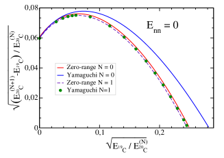
Figure 1: Scaling plots for the first and the second cycles, with $E_{nn}=0$. The range effect in the scaling plot given by the Yamaguchi potential disappears in the second cycle, i.e. $N=1$.

(b) Three-body scaling plot for $E_{nn}=-143\,\text{keV}$

In this section we have presented our results for realistic case, when $E_{nn}=-143$ keV. As it can be verified from our formulation, for large values of parameter $\beta$, the coupled Faddeev equations for Yamaguchi potential goes to zero-range equations. As we can see in Fig. 2, the scaling plot for Yamaguchi potential for high values of $\beta$, or low values of range, is almost the same with zero-range results. This is very useful test to numerically verify the validity of our calculations.

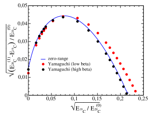
Figure 2: Scaling plots for zero-range and Yamaguchi potentials, with $E_{nn}=-143$ keV. The scaling plot for the Yamaguchi potential goes to zero-range results for large values of $\beta$ (lower values of the effective range).

(c) Effective range correction

The correlation between the binding energy of two successive three-body states is given by a scaling function varying with the energies and ranges of the subsystems. By choosing a very small range for the $nn$ subsystem, one can expand the scaling function in terms of the range of the $nc$ subsystem, i. e. $x_{nc}=r_{nc}\sqrt{2\mu_{nc}E_{nnc}^{(N)}}$. For leading order expansion one can have

$$\dfrac{E_{nnc}^{(N+1)}}{E_{nnc}^{(N)}} = \epsilon\left(-\sqrt{\dfrac{E_{nn}}{E_{nnc}^{(N)}}},\sqrt{\dfrac{E_{nc}}{E_{nnc}^{(N)}}},r_{nn}\sqrt{2\,\mu_{nn}\,E_{nnc}^{(N)}},r_{nc}\sqrt{2\,\mu_{nc}\,E_{nnc}^{(N)}}\right)$$ (10)

$$= \epsilon\left(-\sqrt{\dfrac{E_{nn}}{E_{nnc}^{(N)}}},\sqrt{\dfrac{E_{nc}}{E_{nnc}^{(N)}}}\right)+\dfrac{\delta\epsilon}{\delta x_{nc}}r_{nc}\sqrt{2\,\mu_{nc}\,E_{nnc}^{(N)}}$$ (11)

In Fig 3 we show the results for the derivative $\dfrac{\delta\epsilon}{\delta x_{nc}}r_{nc}$ of this scaling function in terms of the energy of the $nc$ subsystem. Our preliminary results were computed using large values of $\beta$ for $nn$ interaction, while for the $nc$ potential we use for low $\beta$ values. We compute the range effect in Fig 3, which comes essentially from the $nc$ interaction, as the large values of $\beta$ for the $nn$ potential gives small effective range. Our calculation is done for the Yamaguchi potential, and should be viewed as a preliminary calculation, indicating the range correction pattern in the scaling plot of Fig. 2. We have only looked to the range effect in the $nc$ potential, and with a particular form factor for the separable potential. We intend to study different form factors, in order to implement the range correction directly in the set of renormalised subtracted zero-range integral equation. This will allow us to obtain a model independent analysis of the range corrections in the energy scaling plots, namely the correlation between the energy of two close states. Other properties as sizes and momentum distribution should also be investigated in the future.

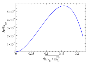
Figure 3: The derivation of ${}^{20}C$ scaling plot, given in Eq. (10), for $E_{nn}=$-143 keV as a function of the $nc$ subsystem energy.

We acknowledge partial financial support from the Brazilian agencies FAPESP, CNPq and CAPES.

References

• (1) V. Efimov, Phys. Lett. B 33, 563 (1970); Nucl. Phys. A 210, 157 (1973).
• (2) A.E.A. Amorim, T. Frederico, L. Tomio, Phys. Rev. C 56, R2378 (1997).
• (3) M. T. Yamashita, T. Frederico, L. Tomio, Phys. Lett. B 660, 339 (2008).
• (4) D. L .Canham and H. Hammer, Eur. Phys. J. A 37, 367 (2008)
• (5) T. Frederico, A. Delfino, L. Tomio, M. T. Yamashita, Prog. Part. Nucl. Phys. 67, 939(2012).
• (6) D. R. Phillips, Few-Body Syst. 55, 931 (2014).
• (7) D. R. Phillips, Pramana 83, 661 (2014).
• (8) T. Frederico, L. Tomio, A. Delfino, M. R. Hadizadeh, M. T. Yamashita, Few-Body Syst. 51, 87 (2011).
• (9) Y. Yamaguchi, Phys. Rev. 95, 1628 (1954).