Ground-state properties of the triangular-lattice Heisenberg antiferromagnet with arbitrary spin quantum number $s$

Abstract

We apply the coupled cluster method to high orders of approximation and exact diagonalizations to study the ground-state properties of the triangular-lattice spin-$s$ Heisenberg antiferromagnet. We calculate the fundamental ground-state quantities, namely, the energy $e_{0}$, the sublattice magnetization $M_{\rm sub}$, the in-plane spin stiffness $\rho_{s}$ and the in-plane magnetic susceptibility $\chi$ for spin quantum numbers $s=1/2,1,\ldots,s_{\rm max}$, where $s_{\rm max}=9/2$ for $e_{0}$ and $M_{\rm sub}$, $s_{\rm max}=4$ for $\rho_{s}$ and $s_{\rm max}=3$ for $\chi$. We use the data for $s\geq 3/2$ to estimate the leading quantum corrections to the classical values of $e_{0}$, $M_{\rm sub}$, $\rho_{s}$, and $\chi$. In addition, we study the magnetization process, the width of the 1/3 plateau as well as the sublattice magnetizations in the plateau state as a function of the spin quantum number $s$.

I Introduction

In the 1970s Anderson and FazekasAnd ; Faz first considered the quantum spin-$1/2$ Heisenberg antiferromagnet (HAFM) for the geometrically frustrated triangular lattice and they proposed a liquid-like ground state (GS) without magnetic long-range order (LRO). Later on it was found that the spin-$1/2$ HAFM on the triangular lattice possesses semi-classical three-sublattice Néel order, see, e.g., Refs. jolicoeur1989 ; bernu1992 ; miyaka1992 ; chub94 ; bernu1994 ; bernu1995 ; manuel1998 ; capriotti1999 ; trumper00 ; ccm_previous ; farnell2001 ; krueger2006 ; weihong2006 ; white2007 ; zhito2009 ; bishop2009 ; zhito2012 . However, the sublattice magnetization $M_{\rm sub}$ is drastically diminished in the $s=1/2$ model capriotti1999 ; krueger2006 ; weihong2006 ; white2007 ; zhito2009 ; bishop2009 because of the interplay between quantum fluctuations and strong frustration. The small magnetic order parameter indicates that the semi-classical magnetic LRO is fragile and that small additional terms in the Hamiltonian may destroy the magnetic LRO, see, e.g., Refs. cheng2011 ; serbyn2011 ; xu2012 ; bieri2012 ; extended1 ; extended2 ; extended3 ; extended4 ; extended5 .

Although very precise data for the relevant GS quantities are available for unfrustrated HAFM’s on bipartite two-dimensional lattices, see, e.g., Refs. qmc1991 ; swt3rd ; lin2001 ; ccm_square2007 related to the square lattice, the corresponding data for the triangular lattice are less precise. This lack of precision is related to the strong frustration in the system that, e.g., does not allow one to apply the quantum Monte Carlo method. Moreover, the spin-wave approach is less efficient for frustrated lattices than it is for non-frustrated lattices. Nevertheless, spin-wave theories are considered as appropriate, in particular, if the spin quantum number $s$ is not $s=1/2$ or $s=1$. Perhaps the most accurate result for the GS order parameter (i.e., the sublattice magnetization $M_{\rm sub}$) for $s=1/2$ has been obtained by a recent density matrix renormalization group study white2007 , where a result of $M_{\rm sub}=0.205$ has been found.

The continuous interest in the triangular-lattice HAFM is (last but not least) also related to a fluctuation-induced magnetization plateau at 1/3 of the saturation magnetization kawa ; nishi ; chub_gol ; Hon1999 ; ono2003 ; HSR04 ; farnell2009 ; alicea ; tay2010 ; zhito2011 ; zhito2011a ; shirata2011 ; shirata2012 ; wir_und_tanaka2013 ; satoshi2013 ; balents2013 ; tanaka2013a ; chub2014 ; zhito2014 ; danshita2014 ; batista2015 . In particular, two model compounds, namely Ba₃CoSb₂O₉ with $s=1/2$ and Ba₃NiSb₂O₉ with $s=1$, have been shown very recently to demonstrate an excellent agreement between the experimentally measured magnetization curves and those curves from theoretical predictions, see Refs. farnell2009 ; shirata2012 ; tanaka2013a for $s=1/2$ and Refs. shirata2011 ; wir_und_tanaka2013 for $s=1$.

In the present paper we consider the Hamiltonian

$$H=\sum_{\langle ij\rangle}{\bf s}_{i}{\bf s}_{j}-h\sum_{i}s_{i}^{z},$$ (1)

where the sum runs over nearest-neighbor bonds ${\langle ij\rangle}$ on the triangular lattice, $({\bf s}_{i})^{2}=s(s+1)$, and $h$ is an external magnetic field. We consider arbitrary spin quantum number $s$. We use the coupled cluster method (CCM) to high orders of approximation to determine the GS properties in zero magnetic field, i.e., the GS energy per spin $e_{0}$, the sublattice magnetization $M_{\rm sub}$ (order parameter), the spin stiffness $\rho_{s}$, and the uniform susceptibility $\chi$. These quantities constitute the fundamental parameters determining the low-energy physics of the triangular Heisenberg antiferromagnet. Moreover, the stiffness and the susceptibility are used as input parameters in scaling functions for various observables chub94_scal .

In addition to the zero-field quantities we also consider the magnetization process $M(h)$ and determine the $1/3$ plateau in the $M(h)$-curve. We complement the CCM calculations by carrying out Lanczos exact diagonalization of finite lattices.

Figure 1: Reference states used for the CCM calculations.

II Methods

II.1 Lanczos exact diagonalization

The Lanzcos exact diagonaliazion (ED) is one of the most useful methods that can be used to investigate frustrated quantum spin systems, see, e.g., Refs. bccj1j2 ; star ; ED40 ; Lauchli ; lauchli2006 ; nakano2013 ; Sakai ; capponi2013 . Although lattices of size $N=36$ are common for ED calculations for spin $s=1/2$, the system size $N$ accessible for ED shrinks significantly, see, e.g., Refs. hida2002 ; lauchli2006 ; nakano2013 ; Lauchli_s1 ; wir_und_tanaka2013 ; Sakai2015 . Hence, we use the ED here in order to complement the results of the CCM (that yields results in the limit $N\to\infty$). We use J. Schulenburg’s spinpack codespinpack to calculate the magnetization curves for $s=1/2,1,\ldots,5/2$. The maximum lattice size for $s=2$ and $5/2$ is $N=12$, whereas for $s=3/2$ we have results for $N=12,18,21$. For $s=1$ the largest lattice we can consider is $N=27$. We use these data to analyze the $s$-dependence of the $1/3$ plateau.

II.2 Coupled cluster method

The coupled cluster method (CCM) is a universal many-body method widely used in various fields of quantum many-body physics, see, e.g. Refs. bartlett97 ; bishop98 . Meanwhile, the CCM has been established as an effective tool in the theory of frustrated quantum spin systems, see, e.g., the recent papers ccm_ferri ; krueger2006 ; Schm:2006 ; rachid08 ; bishop08 ; ccm_odd_even ; farnell2009 ; richter2010 ; farnell11 ; ccm_kago ; wir_und_tanaka2013 ; trian_s1_ccm ; archimedean2014 ; extended4 ; jiang2015 ; kago_xxz . Here we illustrate only some features of the CCM relevant for the present paper. For more general information on the methodology of the CCM, see, e.g., Refs. ccm_roger1990 ; zeng98 ; bishop98 ; bishop00 ; farnell02 ; bishop04 .

The CCM calculation starts with the choice of a normalized reference state $|\Phi\rangle$. We choose the classical GS of the model as reference state, which is well known for the triangular HAFM for arbitrary fields, see, e.g., Refs. chub_gol ; alicea ; farnell2009 and Fig. 1. For zero field it is three-sublattice Néel state, i.e., state I with $\alpha=60^{o}$ in Fig. 1. For finite magnetic fields non-collinear planar states with field dependent pitch angles $\alpha$ and $\beta$ are classical GS’s, see Fig. 1. The reference state is a collinear state (so-called up-up-down state, see state II in Fig. 1) only at the 1/3 plateau. With respect to the corresponding reference state, we then define a set of mutually commuting multispin creation operators $C_{I}^{+}$, which are themselves defined over a complete set of many-body configurations $I$. We perform a rotation of the local axis of the spins such that all spins in the reference state align along the negative $z$ axis. The specific form of the spin-operator transformation depends on the pitch angles of the reference state. In this new set of local spin coordinates the reference state and the corresponding multispin creation operators $C_{I}^{+}$ are given by

$$|{\hat{\Phi}}\rangle=|\downarrow\downarrow\downarrow\cdots\rangle;\mbox{ }C_{I}^{+}={\hat{s}}_{n}^{+}\,,\,{\hat{s}}_{n}^{+}{\hat{s}}_{m}^{+}\,,\,{\hat{s}}_{n}^{+}{\hat{s}}_{m}^{+}{\hat{s}}_{k}^{+}\,,\,\ldots\;,$$ (2)

where the indices $n,m,k,\ldots$ denote arbitrary lattice sites. In the rotated coordinate frame the Hamiltonian becomes dependent on the pitch angles. With the set $\{|\Phi\rangle,C_{I}^{+}\}$ the CCM parametrization of the exact ket and bra GS eigenvectors $|\Psi\rangle$ and $\langle\tilde{\Psi}|$ of the many-body system is given by

$$|\Psi\rangle=e^{S}|\Phi\rangle\;,\mbox{ }S=\sum_{I\neq 0}a_{I}C_{I}^{+}\;$$ (3)

$$\langle\tilde{\Psi}|=\langle\Phi|\tilde{S}e^{-S}\;,\mbox{ }\tilde{S}=1+\sum_{I\neq 0}\tilde{a}_{I}C_{I}^{-}\;,$$ (4)

where $C_{I}^{-}=\left(C_{I}^{+}\right)^{\dagger}$. The CCM correlation operators, $S$ and $\tilde{S}$, contain the correlation coefficients, $a_{I}$ and $\tilde{a}_{I}$, which can be determined by the CCM ket-state and bra-state equations

$$\langle\Phi|C_{I}^{-}e^{-S}He^{S}|\Phi\rangle=0\;\;;\;\forall I\neq 0$$ (5)

$$\langle\Phi|{\tilde{S}}e^{-S}[H,C_{I}^{+}]e^{S}|\Phi\rangle=0\;\;;\;\forall I\neq 0.$$ (6)

Note that each ket-state equation belongs to a specific creation operator
$C_{I}^{+}=s_{n}^{+},\,\,s_{n}^{+}s_{m}^{+},\,\,s_{n}^{+}s_{m}^{+}s_{k}^{+},\cdots$, i.e., it corresponds to a specific set (configuration) of lattice sites $n,m,k,\dots\;.$ By using the Schrödinger equation, $H|\Psi\rangle=E|\Psi\rangle$, we can write the GS energy as $E=\langle\Phi|e^{-S}He^{S}|\Phi\rangle$. The sublattice magnetization is given by $M_{\rm sub}=-(1/N)\sum_{i}^{N}\langle\tilde{\Psi}|s_{i}^{z}|\Psi\rangle$, where $s_{i}^{z}$ is expressed in the transformed coordinate system. The total magnetization $M$ aligned in the direction of the applied magnetic field $h$ in terms of the global axes prior to rotation of the local spin axes is given by $M=(M_{A}+M_{B}+M_{C})/3$, where $M_{A}$, $M_{B}$, and $M_{C}$ are the magnetizations of the three individual sublattices, cf. Fig. 1, given by

$$M_{A,B,C}=\frac{1}{N_{A,B,C}}\sum_{i_{A,B,C}}\langle\tilde{\Psi}|s_{i_{A,B,C}}^{z}|\Psi\rangle,$$ (7)

where the index $i_{A}$ runs over all $N_{A}$ sites on sublattice $A$, the index $i_{B}$ runs over all $N_{B}$ sites on sublattice $B$, and the index $i_{C}$ runs over all $N_{C}$ sites on sublattice $C$, and $N=N_{A}+N_{B}+N_{C}$. The CCM results for the ground state energy and the total magnetization as a function of the magnetic field can be used to calculate the uniform magnetic susceptibility, given by

$$\chi\equiv\frac{dM}{dh}=-\frac{1}{N}\frac{d^{2}E}{dh^{2}}\;.$$ (8)

Note that we consider here $\chi$ as susceptibility per site defin_chi .

The GS energy depends (in a certain CCM approximation, see below) on the pitch angles. In the quantum model the pitch angles may be different to the corresponding classical values. Therefore, we do not choose the classical result for the pitch angles in the quantum model. Indeed, we consider them as a free parameter in the CCM calculation, which has to be determined by minimization of the CCM GS energy with respect to the pitch angles. An exception is the zero-field case, where the pitch angle is fixed to $\alpha=60^{o}$ (the three-sublattice Néel state).

The spin stiffness $\rho_{s}$ measures the increase of energy rotating the order parameter of a magnetically long-range ordered system along a given direction by a small twist (pitch) angle $\theta$ per unit length, i.e.,

$$\frac{E(\theta)}{N}=\frac{E(\theta=0)}{N}+\frac{1}{2}\rho_{s}\theta^{2}+{\cal O}(\theta^{4}),$$ (9)

where $E(\theta)$ is the ground-state energy as a function of the twist angle. For the triangular lattice the twist is imposed along a lattice basis vector and it is within the plane defined by the order parameter, see Refs. bernu1995 ; manuel1998 , where the twist along both directions leads to identical results comment_twist .

For the many-body quantum system under consideration it is necessary to use approximation schemes in order to truncate the expansions of $S$ and $\tilde{S}$ in Eqs. (3) and (4) in a practical calculation. We use the well established SUB$n$-$n$ approximation scheme, cf., e.g., Refs. farnell02 ; bishop04 ; Schm:2006 ; krueger2006 ; rachid08 ; bishop08 ; ccm_odd_even ; farnell2009 ; richter2010 ; farnell11 ; ccm_kago ; wir_und_tanaka2013 ; trian_s1_ccm ; archimedean2014 ; extended4 ; jiang2015 ; kago_xxz ; zeng98 ; bishop00 , where the correlation operators contain no more than $n$ spin flips spanning a range of no more than $n$ contiguous lattice sites SUBn-n .

Using an efficient parallelized CCM code cccm we are able to solve the CCM equations up to SUB10-10 for $s=1/2$ (where, e.g., for the zero-field case reference state a set of 1 054 841 coupled ket-state equations has to be solved). For $s>1/2$ the number of CCM equations increases noticeably. Hence, the highest order of approximation is then SUB8-8 (where, e.g., for the susceptibility for $s=3$ a set of 2 179 007 equations has to be solved).

The SUB$n$-$n$ approximation becomes exact only for $n\to\infty$. We extrapolate the ‘raw’ SUB$n$-$n$ data to $n\to\infty$. Much experience exists relating to the extrapolation of the GS energy per site $e_{0}(n)\equiv E(n)/N$, the magnetic order parameter $M_{\rm sub}$, the spin stiffness $\rho_{s}$, and the susceptibility $\chi$. Thus $e_{0}(n)=a_{0}+a_{1}(1/n)^{2}+a_{2}(1/n)^{4}$ is a very well-tested extrapolation ansatz for the GS energy per spin bishop00 ; bishop04 ; Schm:2006 ; bishop08 ; ccm_odd_even ; rachid08 ; archimedean2014 . An appropriate extrapolation rule for the magnetic order parameter of antiferomagnets with GS LRO is $M_{\rm sub}=b_{0}+b_{1}(1/n)+b_{2}(1/n)^{2}$ bishop00 ; bishop04 ; farnell2009 ; trian_s1_ccm ; archimedean2014 . For the stiffness $\rho_{s}$ as well as for the susceptibility $\chi$ we use the same rule as for $M_{\rm sub}$, i.e., $X(n)=c_{0}+c_{1}(1/n)+c_{2}(1/n)^{2}$, $X=\rho_{s},\chi$, which is able to describe the asymptotic behavior of the CCM-SUB$n$-$n$ data for $\rho_{s}$ well, see Refs. krueger2006 ; rachid08 , and $\chi$, see Ref. farnell2009 .

The selection of the SUB$n$-$n$ data included in the extrapolation is a subtle issue. Often it is argued that the lowest-order data (i.e., SUB2-2 and SUB3-3) ought to be excluded from the extrapolation because these points are rather far from the asymptotic regime ccm_kago ; archimedean2014 ; extended4 . This argument is particularly valid for models which include larger-distance exchange bonds (e.g., so-called $J_{1}$-$J_{2}$ models) rachid08 ; bishop08 ; richter2010 ; farnell11 ; extended4 . However, for the triangular Heisenberg antiferromagnet with only nearest-neighbor bonds even the lowest approximation orders fit well to the extrapolation krueger2006 ; farnell2009 ; wir_und_tanaka2013 . Another point is the odd-even problem, i.e., for odd and even numbers $n$ of the SUB$n$-$n$ approximation the extrapolation may have different fit parameters ccm_odd_even ; archimedean2014 . However, this problem occurs primarily for bipartite systems (with collinear reference states, where no odd-numbered spin flips enter the correlation operators $S$ and $\tilde{S}$), whereas for noncollinear reference states (where odd-numbered spin flips are present in $S$ and $\tilde{S}$) relevant for many frustrated systems both, odd and even SUB$n$-$n$, might be combined in one and the same extrapolation formula krueger2006 ; ccm_kago ; archimedean2014 .

In order to fit the data to the extrapolation formulas given above (which contain three unknown parameters), it is desirable (as a rule) to have at least four data points to obtain a robust and stable fit. To obey this rule we apply here the above given extrapolation formulas using (i) even $n=2,4,6,\ldots$ and (ii) odd and even $n=3,4,5,6,7,\ldots$comp_archi . The maximum approximation level SUB$n_{\rm max}$-$n_{\rm max}$ for $s=1/2$ is $n_{\rm max}=10$ for $e_{0}$ and $M_{\rm sub}$ and $n_{\rm max}=9$ for $\chi$ and $\rho_{s}$, whereas for $s>1/2$ we have $n_{\rm max}=8$. In the following we call case (i) ’extra1’ and case (ii) ’extra2’. The difference between both cases can be considered as a measure of accuracy of our CCM results. To illustrate our extrapolation procedure, we present in Fig. 2 the extrapolations of $e_{0}$, $M_{\rm sub}$, $\chi$, and $\rho_{s}$ for $s=1/2$ and $s=1$. Obviously, the extrapolations work very well for $e_{0}$, $M_{\rm sub}$, and $\rho_{s}$, and, both schemes, ’extra1’ and ’extra2’, lead to very similar results. There is some scattering of the SUB$n$-$n$ data only for $\chi$, and, as a consequence, there is a visible difference between the extrapolations ’extra1’ and ’extra2’.

Table 1: Extrapolated CCM results for the GS energy per spin, $e_{0}|_{n\to\infty}$, the GS sublattice magnetization, $M_{\rm sub}|_{n\to\infty}$, the spin stiffness, $\rho_{s}|_{n\to\infty}$, and the susceptibility, $\chi|_{n\to\infty}$. We mention that the spin-wave velocity $c_{\rm swt}$ can be calculated from $\rho_{s}$ and $\chi$ by using the hydrodynamic relation $c^{2}_{\rm swt}=\rho_{s}/\chi$.

extra1 extra2   $e_{0}/s^{2}$   $M_{\rm sub}/s$   $\rho_{s}/s^{2}$   $\chi$   $e_{0}/s^{2}$   $M_{\rm sub}/s$   $\rho_{s}/s^{2}$   $\chi$ $s=1/2$   -2.2056   0.4307   0.3103   0.0652   -2.2045   0.4248   0.2990   0.0553 $s=1$   -1.8384   0.7303   0.6429   0.0956   -1.8367   0.7350   0.6572   0.0902 $s=3/2$   -1.7234   0.8169   0.7636   0.0996   -1.7223   0.8232   0.7757   0.0972 $s=2$   -1.6667   0.8628   0.8246   0.1023   -1.6659   0.8695   0.8342   0.1012 $s=5/2$   -1.6329   0.8909   0.8610   0.1041   -1.6323   0.8973   0.8687   0.1035 $s=3$   -1.6105   0.9096   0.8850   0.1054   -1.6000   0.9155   0.8913   0.1050 $s=7/2$   -1.5946   0.9229   0.9019  -   -1.5941   0.9282   0.9071  - $s=4$   -1.5826   0.9328   0.9145  -   -1.5823   0.9376   0.9188  - $s=9/2$   -1.5734   0.9404  -  -   -1.5731   0.9448  -  -

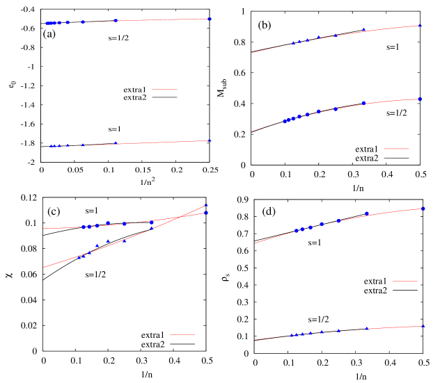
Figure 2: Extrapolation of the CCM-SUB$n$-$n$ for the GS energy $e_{0}$ (a), the sublattice magnetization $M_{\rm sub}$ (b), the susceptibility $\chi$ (c), and the spin stiffness $\rho_{s}$ (d) for spin quantum numbers $s=1/2$ and $1$ using two different extrapolation schemes (labeled by ’extra1’ and ’extra2’), cf. main text.

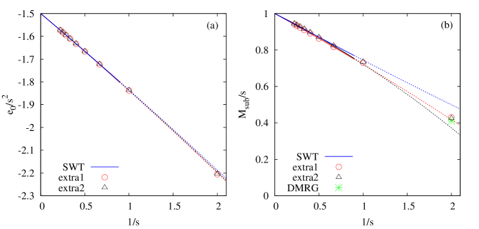
Figure 3: Extrapolated CCM data (schemes ’extra1’ and ’extra2’, see main text) as a function of $1/s$ compared with higher-order spin-wave theory (SWT, blue line) taken from Ref.zhito2009 . The symbols represent the CCM data points, the corresponding red and black lines show the fit function $X(s)=X|_{s\to\infty}\left(1-x_{1}/s-x_{2}/s^{2}\right)$, where the data for $s\geq 3/2$ were used for the fit. (a): GS energy $e_{0}$. (b) Sublattice magnetization $M_{\rm sub}$ (the green symbol shows the density matrix renormalization group result (DMRG) for $s=1/2$ from Ref. white2007 ).

Table 2: Parameters $x_{1}$ and $x_{2}$ of the $1/s$ expansion $X(s)=X|_{s\to\infty}\left(1-x_{1}/s-x_{2}/s^{2}\right)$ obtained from the extrapolated CCM results for the GS energy $e_{0}$, the sublattice magnetization $M_{\rm sub}$, the spin stiffness $\rho_{s}$ and the susceptibility $\chi$.

$e_{0}$ $M_{\rm sub}$   $x_{1}$   $x_{2}$   $x_{1}$   $x_{2}$ extra1   0.2176   0.0071   -0.2671   -0.0120 extra2   0.2186   0.0073   -0.2416   -0.0362 $\rho_{s}$ $\chi$   $x_{1}$   $x_{2}$   $x_{1}$   $x_{2}$ extra1   -0.3355   -0.0292   -0.1587   0.0045 extra2   -0.3166   -0.0297   -0.1440   -0.0662

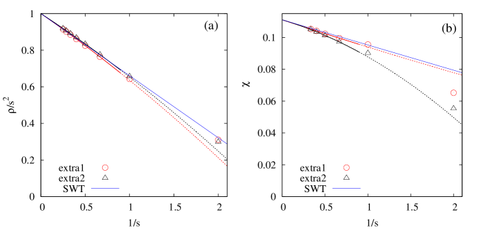
Figure 4: Extrapolated CCM data (schemes ’extra1’ and ’extra2’, see main text) for the spin stiffness $\rho_{s}$ (a) and the susceptibility $\chi$ (b) as a function of $1/s$ compared with spin-wave theory (SWT, blue line) taken from Ref. bernu1995 (for $\rho_{s}$) and Ref. chub94 (for $\chi$). The symbols represent the CCM data points, the corresponding red and black lines show the fit function $X(s)=X|_{s\to\infty}\left(1-x_{1}/s-x_{2}/s^{2}\right)$, where for the fit the data for $s\geq 3/2$ were used.

III Results

III.1 The zero-field case

In this section we present CCM results for the GS energy per spin $e_{0}$, the sublattice magnetization $M_{\rm sub}$ (order parameter), the spin stiffness $\rho_{s}$, and the uniform susceptibility $\chi$ for spin quantum numbers $s=1/2,1,\ldots,9/2$ (for $e_{0}$ and $M_{\rm sub}$), for $s=1/2,1,\ldots,4$ (for $\rho_{s}$ ), and for $s=1/2,1,\ldots,3$ (for $\chi$). Moreover, we use the data for $s\geq 3/2$ to estimate the leading quantum corrections to the classical values to compare with the $1/s$ spin-wave expansion bernu1995 ; miyaka1992 ; chub94 ; zhito2009 .

The data for the GS energy and the sublattice magnetization are collected in Table 1. The difference between both extrapolation schemes, ’extra1’ and ’extra2’, is largest for lower spin quantum numbers $s$, although it is still small for all values of $s$. In the extreme quantum limit $s=1/2$ the density matrix renormalization group result white2007 $M_{\rm sub}/s=0.410$ is slightly lower than our CCM result.

Let us now compare our data for $e_{0}$ and $M_{\rm sub}$ with recent higher-order spin-wave results by Chernyshev and Zhitomirsky zhito2009 . Chernyshev and Zhitomirsky found that $e_{0}(s)=-1.5s^{2}(1+0.218412/s+0.0053525/s^{2})$ and $M_{\rm sub}(s)=s(1-0.261303/s+0.0055225/s^{2})$. We fit our extrapolated CCM data for $s=3/2,2,\ldots,9/2$ using the ansatz
$X(s)=X|_{s\to\infty}\left(1-x_{1}/s-x_{2}/s^{2}\right)$, $X=e_{0},M_{\rm sub}$. The classical values are $e_{0}|_{s\to\infty}=-3s^{2}/2$, and $M_{\rm sub}|_{s\to\infty}=s$.

The values for the $1/s$ expansion parameters $x_{1}$ and $x_{2}$ are listed in Table 2 and the corresponding results are depicted in Fig. 3. For the GS energy $x_{1}$ and $x_{2}$ are in very good agreement with the spin-wave results zhito2009 . The leading coefficient $x_{1}$ for the order parameter also fits well to the spin-wave term. However, we obtain (small) negative values instead of a (small) positive one for the next-order coefficient $x_{2}$. The good agreement between the spin-wave and the CCM results for the GS energy is also evident in Fig. 3(a). Moreover, the $1/s$ expansion up to second order yields reasonable results for $e_{0}$ even for the extreme quantum case $s=1/2$. On the other hand, the deviation for the sublattice magnetization becomes noticeable for $s<3/2$, see Fig. 3(b). Thus, by contrast to the GS energy, the $1/s$ expansion of $M_{\rm sub}/s$ up to order $s^{-2}$ leads to values for $s=1/2$ with limited accuracy. We know that the sublattice magnetization of the unfrustrated square-lattice $s=1/2$ Heisenberg antiferromagnet obtained by higher-order spin-wave theoryswt3rd agrees well with quantum Monte Carloqmc1991 and CCMccm_square2007 results. Thus the deviation for the triangular lattice might be attributed to the enhanced quantum fluctuations caused by frustration leading to a particularly small value of $M_{\rm sub}$ for $s=1/2$.

Next we discuss the in-plane spin stiffness $\rho_{s}$ and the in-plane magnetic susceptibility $\chi$. Results are given in Table 1. As already mentioned above, the extrapolation of the CCM-SUB$n$-$n$ data works well for $\rho_{s}$, although it is less accurate for $\chi$, i.e. for $\chi$ the deviation between the schemes ’extra1’ and ’extra2’ is noticeable, cf. Table 1 and Fig. 2. The spin-wave large-$s$ relations are $\rho_{s}=s^{2}(1-0.3392/s)$ (Ref. bernu1995 ) and $\chi=(1/9)(1-0.1425/s)$ (Ref. chub94 ). Fitting the data from Table 1 for $s\geq 3/2$ using the ansatz $X(s)=X|_{s\to\infty}\left(1-x_{1}/s-x_{2}/s^{2}\right)$, $X=\rho_{s},\chi$, $\rho_{s}|_{s\to\infty}=s^{2}$, and $\chi|_{s\to\infty}=1/9$, gives values for the $1/s$ expansion parameters $x_{1}$ and $x_{2}$ which are listed in Table 2. The leading coefficient $x_{1}$ fits reasonably well to the spin-wave term. The deviation between the schemes ’extra1’ and ’extra2’ for $\chi$ results in different signs of the second-order term $x_{2}$. We show the $1/s$ dependence of $\rho_{s}$ and $\chi$ in Fig. 4. It is obvious that the large-$s$ approach works surprisingly well for $\rho_{s}$ down to $s=1/2$, whereas it seems to fail for $\chi$ for $s=1/2$.

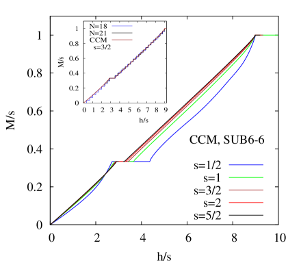
Figure 5: Main: The magnetization curve calculated within CCM-SUB6-6 approximation for $s=1/2,1,3/2,2$ and $5/2$. Inset: The magnetization curve for $s=3/2$ calculated with exact diagonalization for finite lattices of $N=18$ and $21$ sites compared with the CCM-SUB6-6 data.

III.2 The magnetization process

As already mentioned in the introduction, the magnetization process $M(h)$ for $s=1/2$ was investigated previously in numerous papers nishi ; chub_gol ; Hon1999 ; HSR04 ; farnell2009 ; tay2010 ; zhito2011 ; shirata2012 ; satoshi2013 ; balents2013 ; tanaka2013a ; zhito2014 ; danshita2014 ; batista2015 . The $M(h)$ curve for the specific case $s=1$ was much less studied nakano2013 ; wir_und_tanaka2013 . Several quasi-classical large-$s$ approacheschub_gol ; alicea ; zhito2011 ; zhito2014 ; chub2014 can be used to obtain an estimate for $M(h)$ and the $1/3$ plateau also for lower spin quantum numbers. However, it is likely that these results have limited accuracy (see also the discussion in Sec. III.1). We mention again that very good agreement between experimental and theoretical CCM data for $s=1/2$ and $s=1$ has been reported shirata2012 ; wir_und_tanaka2013 very recently.

Let us mention that the CCM calculations of the $M(h)$ curves are extremely time consuming, because the field dependent quantum pitch angles for each value of the magnetic field have to be determined by minimization of the CCM-SUB$n$-$n$ GS energy with respect to the pitch angles. Hence we consider only even SUB$n$-$n$ approximations until $n=6$. We have data for SUB8-8 only for the critical fields, $h_{c1}$ and $h_{c2}$, which bound the $1/3$ plateau, and only for the most interesting extreme quantum cases of $s=1$ and $s=1/2$. We show the CCM-SUB6-6 magnetization curves for $s=1/2,1,3/2,2$, and $5/2$ in the main panel of Fig. 5. The width of the $1/3$ plateau shrinks with increasing spin quantum number $s$ which is clearly seen in Fig. 5. From the experimental point of view this shrinking of the plateau width is relevant. Thus for $s=2$ the plateau width $(h_{c2}-h_{c1})/s$ is only about $25\%$ of the width for $s=1/2$ which makes its detection for large $s$ by measurements at low (but finite) temperatures more challenging. From Fig. 5 it is obvious that all curves for $s>1/2$ are close to each other. Below and above the plateau they show almost the classical linear $h$ dependence of $M$. The $s=1/2$ curve is well separated and shows a pronounced deviation from linearity. The curves shown in the inset demonstrate that CCM and ED data agree well.

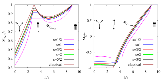
Figure 6: Field dependence of the sublattice magnetizations $M_{A}=M_{B}$ (left) and $M_{C}$ (right), cf. Fig. 1, calculated within CCM-SUB6-6 approximation for $s=1/2,1,3/2,2$ and $5/2$.

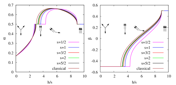
Figure 7: Field dependence of the pitch angles $\alpha$ (left) and $\beta$ (right), cf. Fig. 1, calculated within CCM-SUB6-6 approximation for $s=1/2,1,3/2,2$ and $5/2$.

The CCM approach allows to calculate the individual sublattice magnetizations $M_{A}=M_{B}$ and $M_{C}$ as well as the quantum pitch angles $\alpha$ and $\beta$, cf. Fig. 1. These quantities, are accessible, in principle, in neutron scattering experiments. They provide a deeper insight in the details of the magnetization process and the role of quantum fluctuations. We show $M_{A},M_{B}$ and $M_{C}$ in Fig. 6 and $\alpha$ and $\beta$ in Fig. 7. An interesting feature is the non-monotonic behavior of $M_{C}$ for $h<h_{c1}$ (present only in the quantum model) and of $M_{A},M_{B}$ and $\alpha$ above the plateau. There is a strong increase in the slopes (except for $M_{C}$ and $\beta$ near $h_{c1}$) as one one approaches the plateau from below or above.

For the collinear plateau state at one third of the saturation (the so-called ’up-up-down’ state, see state II in Fig. 1) we have calculated SUB$n$-$n$ data of the sublattice magnetizations $M_{\rm up}=M_{A}=M_{B}$ and $M_{\rm down}=M_{C}$ up to $n_{\rm max}=10$ for $s=1/2$ and $1$ and up to $n_{\rm max}=8$ for $s=3/2,2,\dots,4$. Again we perform an extrapolation of the CCM-SUB$n$-$n$ data applying $M_{X}=b_{0}+b_{1}(1/n)+b_{2}(1/n)^{2}$, $X=A,B,C$. We use only even SUB$n$-$n$ approximations for the extrapolation and the corresponding scheme is therefore ’extra1’ (see Sec. II.2). The resulting data for $M_{A}=M_{B}$ and $M_{C}$ are given in Table 3. We find that $M_{\rm up}$ is always larger than $|M_{\rm down}|$. In particular, the difference in the magnitude of both quantities is remarkably large for $s=1/2$. As for the zero-field case, the sublattice magnetizations within the plateau state are reduced by quantum fluctuations. This reduction is, however, much smaller than that for the canted zero-field state.

We obtain the $1/s$ dependence for $M_{A}=M_{B}$ and $M_{C}$ by fitting our extrapolated CCM data for $s\geq 3/2$ using (as previously) the ansatz $X(s)=X|_{s\to\infty}\left(1-x_{1}/s-x_{2}/s^{2}\right)$, $X=M_{A,B,C}$. The classical values are $M_{A,B}|_{s\to\infty}=s$ and $M_{C}|_{s\to\infty}=-s$. The values for $1/s$ expansion parameters $x_{1}$ and $x_{2}$ are $x_{1}=-0.1003$ and $x_{2}=0.0091$ for $M_{A,B}$ and $x_{1}=+0.2006$ and $x_{2}=-0.0182$ for $M_{C}$ and the corresponding $1/s$ behavior is shown in Fig. 8.

Table 3: Extrapolated CCM results (extrapolation scheme ’extra1’) for the sublattice magnetizations in the plateau state, $M_{X}|_{n\to\infty}$, $X=A,B,C$.

  $s=1/2$   $s=1$   $s=3/2$   $s=2$   $s=5/2$   $s=3$   $s=7/2$   $s=4$ $M_{A,B}$   0.8392   0.9095   0.9372   0.9521   0.9614   0.9676   0.9721   0.9755 $M_{C}$   -0.6783   -0.8190   -0.8743   -0.9043   -0.9227   -0.9352   -0.9441   -0.9509

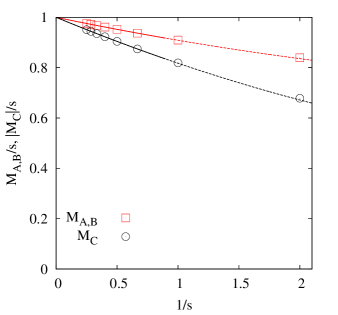
Figure 8: Extrapolated CCM data (scheme ’extra1’, see main text) for the sublattice magnetizations in the plateau state, $M_{A}=M_{B}$ and $M_{C}$, as a function of $1/s$. The symbols represent the CCM data points, the corresponding red and black lines show the fit function $M_{X}(s)=M_{X}|_{s\to\infty}\left(1-x_{1}/s-x_{2}/s^{2}\right)$.

We shall now discuss in some detail the critical fields, $h_{c1}$ and $h_{c2}$, that define the position and the width of the plateau in the $M(h)$ curve. These results are also relevant for the experimental searches of the magetization plateau in magnetic compounds with triangular-lattice structure, cf. Refs. shirata2011 ; shirata2012 ; tanaka2013a ; wir_und_tanaka2013 . We present our data in Table 4 and show the $1/s$ dependences of $h_{c1}$ and $h_{c2}$ in Fig. 9. In addition to our CCM and ED data, we show also relevant data for $h_{c1}$ and $h_{c2}$ from Refs. chub_gol ; zhito2011 ; zhito2014 ; danshita2014 for comparison. The monotonic shrinking of the plateau widths known for the large-$s$ approaches is also clearly seen in our CCM and ED data.

We notice that the plateau ends at $h_{c1}$ and $h_{c2}$ behave differently with increasing $s$. Although the lower plateau end is only slightly shifted, the shift of the upper one at $h_{c2}$ is more pronounced, see also Figs. 5-7. We also see that the data for $h_{c1}$ and $h_{c2}$ provided in the literature for the extreme quantum case $s=1/2$ exhibit a rather large amount of scattering. As already found for the zero-field sublattice magnetization and susceptibility, cf. Sec. III.1, the quasi-classical large-$s$ approaches chub_gol ; zhito2011 ; zhito2014 for $s=1/2$ noticeably deviate from our data directly calculated for $s=1/2$. Moreover, the recent real-space perturbation theoryzhito2014 yields an $1/s$-dependence of $h_{c1}$ and $h_{c2}$ that significantly deviates from the spin-wave, ED as well as the CCM behavior. On the other hand, the recent large-scale cluster mean-field approach of Ref. danshita2014 yields $h_{c1}/s=2.690$ and $h_{c2}/s=4.226$ for the $s=1/2$ case, and these values are close to the CCM-SUB8-8 results.

Table 4: Critical fields $h_{c1}$ and $h_{c2}$, where the one-third plateau begins and ends. Note that for $s=1/2$ ED data also for $N=36$ and $39$ are available Hon1999 ; HSR04 ; Sakai .

CCM SUB2-2 SUB4-4 SUB6-6 SUB8-8 $s$   $h_{c1}/s$   $h_{c2}/s$   $h_{c1}/s$   $h_{c2}/s$   $h_{c1}/s$   $h_{c2}/s$   $h_{c1}/s$   $h_{c2}/s$ $1/2$   2.382   4.344   2.624   4.482   2.714   4.370   2.740   4.290 $1$   2.727   3.617   2.788   3.674   2.809   3.648   2.814   3.637 $3/2$   2.826   3.405   2.854   3.440   2.862   3.429   –   – $2$   2.873   3.303   2.888   3.327   2.892   3.322   –   – $5/2$   2.900   3.242   2.909   3.261   2.911   3.257   –   – $3$   2.917   3.202   2.923   3.217   2.925   3.214   –   – ED $N=12$ $N=18$ $N=21$ $N=27$ $s$   $h_{c1}/s$   $h_{c2}/s$   $h_{c1}/s$   $h_{c2}/s$   $h_{c1}/s$   $h_{c2}/s$   $h_{c1}/s$   $h_{c2}/s$ $1/2$   2.615   4.934   2.805   4.578   2.794   4.425   2.745   4.382 $1$   2.816   3.916   2.879   3.786   2.851   3.717   2.817   3.695 $3/2$   2.864   3.613   2.913   3.523   2.890   3.479   –   – $2$   2.893   3.461   2.932   3.391   –   –   –   – $5/2$   2.911   3.369   –   –   –   –   –   – $3$   2.924   3.308   –   –   –   –   –   –

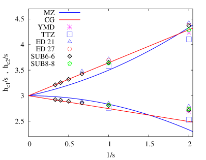
Figure 9: Critical fields, $h_{c1}$ and $h_{c2}$, that bound the $1/3$ plateau versus the inverse of the spin quantum number, $1/s$, calculated by exact diagonalization for $N=21$ and $27$ (labels ED 21 and ED 27) and CCM (labels SUB4-4 and SUB6-6) compared to large-$s$ approaches chub_gol ; zhito2011 ; zhito2014 and cluster mean-field data danshita2014 . The blue lines (labeled by MZ) correspond to $h_{c1}/s=3-1/6s^{2}$ and $h_{c2}/s=3+1/3s+1/6s^{2}$ (Ref. zhito2014 ) and the red lines (labeled by CG) correspond to $h_{c1}/s=3-0.028/s$ and $h_{c2}/s=3+0.0717/s$ (Ref. chub_gol ). The abbreviations YMD and TTZ represent data from Ref. danshita2014 and Ref. zhito2011 , respectively.

IV Summary

The HAFM on the triangular lattice is a basic model of quantum magnetism. The theoretical treatment of this frustrated spin model is challenging and the precision of the existing data for the basic parameters determining the low-energy physics of the model is less than that of corresponding unfrustrated models such as the square-lattice HAFM. Furthermore several magnetic compounds exist, see e.g. Refs. shirata2011 ; shirata2012 ; tanaka2013a ; Nakatsuji2007 ; Reotier2007 ; Bao2009 ; Reotier2015 , that are described by this model. Hence, there is a need to improve the accuracy of the data available from theoretical investigations also from the experimental point of view.

In the present paper we present large-scale CCM calculations for the basic GS parameters, energy $e_{0}$, sublattice magnetization $M_{\rm sub}$, in-plane spin stiffness $\rho_{s}$ and in-plane magnetic susceptibility $\chi$, for arbitrary spin quantum number $s$. In addition to these zero-field quantities, we also consider the magnetization process. It is known from many previous studies for other frustrated quantum spin models, such as the kagome HAFM and the $J_{1}$-$J_{2}$ square-lattice HAFM, that the CCM provides accurate GS results. Hence, the results presented here will contribute to improve available theoretical data, especially for the extreme quantum cases $s=1/2$ and $s=1$ where large-$s$ (spin-wave) theories do not to provide sufficently precise data.

Although the present study is purely theoretical, the data presented here might be used to interpret experimental results for magnetic compounds that are described by the triangular-lattice HAFM, see e.g. Refs. shirata2011 ; shirata2012 ; tanaka2013a ; Nakatsuji2007 ; Reotier2007 ; Bao2009 ; Reotier2015 . As already mentioned above, the compounds Ba₃CoSb₂O₉ and Ba₃NiSb₂O₉ are described well by the Heisenberg model considered here with spin quantum number $s=1/2$ (Ba₃CoSb₂O₉)shirata2012 and $s=1$ (Ba₃NiSb₂O₉)shirata2011 ; wir_und_tanaka2013 . We remark that very good agreement between the theoretical CCM data and experimental data has been reported for these cases. The CCM data presented here for $s=3/2$ and $s=2$ might be useful for further studies of the magnetic compounds La₂Ca₂MnO₇ (with $s=3/2$) Bao2009 ; Reotier2015 and FeGa₂S₄ (with $s=2$) Nakatsuji2007 ; Reotier2007 .

References

- (1) P.W. Anderson, Mater. Res. Bull. 8 153 (1973).
- (2) P. Fazekas, P.W. Anderson, Philos. Mag. 30, 423 (1974).
- (3) T. Jolicoeur and J.C. Le Gouillou, Phys. Rev. B 40, 2727 (1989).
- (4) B. Bernu, C. Lhuillier, L. Pierre, Phys. Rev. Lett. 69, 2590 (1992).
- (5) S.J. Miyake, J. Phys. Soc. Jpn. 61, 983 (1992).
- (6) A. V. Chubukov, S. Sachdev, and T. Senthil, J. Phys.: Condens. Matter 6, 8891 (1994).
- (7) B. Bernu, P. Lecheminant, C. Lhuillier, and L. Piere, Phys. Rev. B 50, 10048 (1994).
- (8) P. Lecheminant, B. Bernu, and C. Lhuillier, Phys. Rev. B 52, 9162 (1995).
- (9) C. Zeng, I. Staples, and R. F. Bishop, Phys. Rev. B 53, 9168 (1996).
- (10) L. O. Manuel, A. E. Trumper, and H. A. Ceccatto, Phys. Rev. B 57, 8348 (1998).
- (11) L. Capriotti, A.E. Trumper, S. Sorella, Phys. Rev. Lett. 82, 3899 (1999).
- (12) A.E. Trumper, L. Capriotti and S. Sorella, Phys. Rev. B 61, 11529 (2000).
- (13) D. J. Farnell, R. F. Bishop, and K. A. Gernoth, Phys. Rev. B 63, 220402 (2001).
- (14) S.E. Krüger, R. Darradi, J. Richter, and D.J.J. Farnell, Phys. Rev. B 73, 094404 (2006).
- (15) Weihong Zheng, J. O. Fjaerestad, R. R. P. Singh, R. H. McKenzie, and Radu Coldea, Phys. Rev. B 74, 224420 (2006).
- (16) S. R. White and A. L. Chernyshev, Phys. Rev. Lett. 99, 127004 (2007).
- (17) A. L. Chernyshev and M. E. Zhitomirsky, Phys. Rev. B 79, 144416 (2009).
- (18) R.F. Bishop, P.H.Y. Li, D.J.J. Farnell, and C.E. Campbell, Phys. Rev. B 79, 174405 (2009).
- (19) M. E. Zhitomirsky and A. L. Chernyshev, Rev. Mod. Phys. 85, 219 (2013).
- (20) J. G. Cheng, G. Li, L. Balicas, J. S. Zhou, J. B. Goodenough, Cenke Xu, and H. D. Zhou, Phys. Rev. Lett. 107, 197204 (2011).
- (21) M. Serbyn, T. Senthil, P. A. Lee, Phys. Rev. B 84, 180403 (2011).
- (22) C. Xu, F. Wang, Y. Qi, L. Balents, M. P. A. Fisher, Phys. Rev. Lett. 108, 087204 (2012).
- (23) S. Bieri, M. Serbyn, T. Senthil, P. A. Lee, Phys. Rev. B 86, 224409 (2012).
- (24) R. V. Mishmash, J. R. Garrison, S. Bieri, and C. Xu, Phys. Rev. Lett. 111, 157203 (2013).
- (25) N. Suzuki, F. Matsubara, S. Fujiki, and T. Shirakura, Phys. Rev. B 90, 184414 (2014).
- (26) R. Kaneko, S. Morita, and M. Imada, J. Phys. Soc. Jpn. 83, 093707 (2014).
- (27) P.H.Y. Li, R.F. Bishop, C.E. Campbell, Phys. Rev. B 91, 014426 (2015).
- (28) Z. Zhu and S.R. White, arXiv:1502.04831.
- (29) M. S. Makivic and H.-Q. Ding, Phys. Rev. B 43, 3562 (1991).
- (30) C.J. Hamer, Zheng Weihong, and P. Arndt, Phys. Rev. B 46, 6276 (1992).
- (31) H.-Q. Lin, J. S. Flynn, and D. D. Betts, Phys. Rev. B 64 214411 (2001).
- (32) J. Richter, R. Darradi, R. Zinke, and R.F. Bishop, Int. J. Modern Phys. B 21, 2273 (2007).
- (33) H. Kawamura and S. Miyashita, J. Phys. Soc. Jpn. 54, 4530 (1985).
- (34) H. Nishimori and S. Miyashita, J. Phys. Soc. Japan 55, 4448 (1986).
- (35) A.V. Chubukov and D.I. Golosov, J. Phys.: Condens. Matter 3, 69 (1991).
- (36) A. Honecker, J. Phys.: Condens. Matter 11, 4697 (1999).
- (37) T. Ono, H. Tanaka, H. Aruga Katori, F. Ishikawa, H. Mitamura, and T. Goto, Phys. Rev. B 67, 104431 (2003).
- (38) A. Honecker, J. Schulenburg, and J. Richter, J. Phys.: Condens. Matter 16, S749 (2004).
- (39) D.J.J. Farnell, R. Zinke, J. Schulenburg, and J. Richter, J. Phys.: Condens. Matter 21, 406002 (2009).
- (40) J. Alicea, A.V. Chubukov, O.A. Starykh, Phys. Rev. Lett. 102, 137201 (2009).
- (41) T. Tay and O.I. Motrunich, Phys. Rev. B 81, 165116 (2010).
- (42) J. Takano, H. Tsunetsugu and M. E. Zhitomirsky, J. Phys.: Conf. Series 320, 012011 (2011).
- (43) M.V. Gvozdikova, P.-E. Melchy and M.E. Zhitomirsky, J. Phys.: Condens. Matter 23 164209 (2011).
- (44) Y. Shirata, H. Tanaka, T. Ono, A. Matsuo, K. Kindo, and H. Nakano, J. Phys. Soc. Japan 80, 093702 (2011).
- (45) Y. Shirata, H. Tanaka, A. Matsuo, and K. Kindo, Phys. Rev. Lett. 108, 057205 (2012).
- (46) T. Susuki, N. Kurita, T. Tanaka, H. Nojiri, A Matsuo, K. Kindo, H. Tanaka, Phys. Rev. Lett. 110, 267201 (2013).
- (47) C. Hotta, S. Nishimoto, and N.Shibata, Phys. Rev. B 87, 115128 (2013).
- (48) J. Richter, O. Götze, R. Zinke, D.J.J. Farnell, and H. Tanaka, J. Phys. Soc. Jpn. 82, 015002 (2013).
- (49) R. Chen, H. Ju, H.-C. Jiang, O.A. Starykh, and L. Balents, Phys. Rev. B 87 165123 (2013).
- (50) O.A. Starykh, W. Jin, and A.V. Chubukov, Phys. Rev. Lett. 113, 087204 (2014).
- (51) D. Yamamoto, G. Marmorini, and I. Danshita, Phys. Rev. Lett. 112, 127203 (2014); Phys. Rev. Lett. 112, 259901 (2014).
- (52) M. E. Zhitomirsky, J. Phys.: Conf. Ser. 592, 012110 (2015).
- (53) G. Koutroulakis, T. Zhou, Y. Kamiya, J. D. Thompson, H. D. Zhou, C. D. Batista, and S. E. Brown, Phys. Rev. B 91, 024410 (2015).
- (54) A. V. Chubukov, T. Senthil, and S. Sachdev, Phys. Rev. Lett. 72, 2089 (1994).
- (55) R. Schmidt, J. Schulenburg, J. Richter, and D.D. Betts, Phys. Rev. B 66, 224406 (2002).
- (56) J. Richter, J. Schulenburg, A. Honecker, and D. Schmalfuß, Phys. Rev. B 70, 174454 (2004).
- (57) A. Läuchli, F. Mila, and K. Penc, Phys. Rev. Lett. 97, 087205 (2006).
- (58) J. Richter and J. Schulenburg, Eur. Phys. J. B 73, 117 (2010).
- (59) A.M. Läuchli, J. Sudan, and E.S. Sorensen, Phys. Rev. B 83, 212401 (2011).
- (60) H. Nakano, S. Todo, and T. Sakai, J. Phys. Soc. Jpn. 82, 043715 (2013).
- (61) T. Sakai and H. Nakano, Phys. Rev. B 83, 100405(R) (2011); J. Phys. Conf. Series 320, 012016 (2011).
- (62) S. Capponi, O. Derzhko, A. Honecker, A. M. Läuchli, and J. Richter, Phys. Rev. B 88, 144416 (2013).
- (63) K. Hida, J. Phys. Soc. Japan 70, 3673 (2002).
- (64) A.M. Läuchli and H.J. Changlani, Phys. Rev. B 91, 100407 (2015).
- (65) H. Nakano and T. Sakai, J. Phys. Soc. Jpn. 84, 063705 (2015).
- (66) http://www-e.uni-magdeburg.de/jschulen/spin/
- (67) Recent Advances in Coupled-Cluster Methods, ed. R.-J. Bartlett (World Scientific, Singapore, 1997).
- (68) R.F. Bishop in Microscopic Many-Body Theories and Their Applications, eds. J. Navarro and A. Polls, Lecture Notes in Physics Vol. 510 (Springer 1998).
- (69) N.B. Ivanov, J. Richter and D.J.J. Farnell, Phys. Rev. B 66, 014421 (2002).
- (70) D. Schmalfuß, R. Darradi, J. Richter, J. Schulenburg, and D. Ihle, Phys. Rev. Lett. 97, 157201 (2006).
- (71) R. Darradi, O. Derzhko, R. Zinke, J. Schulenburg, S. E. Krüger and J. Richter, Phys. Rev. B 78, 214415 (2008).
- (72) R. F. Bishop, P. H. Y. Li, R. Darradi, and J. Richter, J. Phys.: Condens. Matter 20, 255251 (2008).
- (73) D.J.J. Farnell and R.F. Bishop, Int. J. Modern Phys. B 22, 3369 (2008).
- (74) J. Richter, R. Darradi, J. Schulenburg, D. J. J. Farnell, and H. Rosner, Phys. Rev. B 81, 174429 (2010).
- (75) D. J. J. Farnell, R. F. Bishop, P. H. Y. Li, J. Richter, and C. E. Campbell, Phys. Rev. B 84, 012403 (2011).
- (76) O. Götze, D.J.J. Farnell, R.F. Bishop, P.H.Y. Li, and J. Richter, Phys. Rev. B 84, 224428 (2011).
- (77) P.H.Y. Li and R.F. Bishop, Eur. Phys. J B 85, 25 (2012).
- (78) D.J.J. Farnell, O. Götze, J. Richter, R.F. Bishop, and P.H.Y. Li, Phys. Rev. B 89, 184407 (2014).
- (79) J.-J. Jiang, Y.-J Liu, F. Tang, C.-H. Yang, and Y.-B. Sheng, Physica B: Cond. Mat. 463, 30 (2015).
- (80) O. Götze and J. Richter, Phys. Rev. B 91, 104402 (2015).
- (81) M. Roger and J.H. Hetherington, Phys. Rev. B 41, 200 (1990); Europhys. Lett. 11, 255 (1990).
- (82) C. Zeng, D. J. J. Farnell, and R. F. Bishop, J. Stat. Phys. 90, 327 (1998).
- (83) R. F. Bishop, D. J. J. Farnell, S. E. Krüger, J. B. Parkinson, J. Richter, and C. Zeng, J. Phys.: Condens. Matter 12, 6887 (2000).
- (84) D. J. J. Farnell, R. F. Bishop and K. A. Gernoth, J. Stat. Phys. 108, 401 (2000).
- (85) D. J. J. Farnell and R. F. Bishop, in Quantum Magnetism, Lecture Notes in Physics 645, edited by U. Schollwöck, J. Richter, D. J. J. Farnell, and R. F. Bishop (Springer, Berlin, 2004), p. 307.
- (86) is sometimes defined per volume, see e.g. Ref. chub94 , which yields a factor of for the triangular lattice.
- (87) Note that the definition of the twist used in the present paper following Refs. bernu1995 ; manuel1998 is slightly different from that used in Ref. krueger2006 , where the CCM was used to calculate the triangular-lattice GS energy for as a function of the twist angle up to order SUB7-7.
- (88) Note that the notation LSUB is used for typically, see, e.g., Ref. farnell2009 . Thus we mention here that for the LSUB scheme is identical to the SUB- scheme.
- (89) We use the program package ‘The crystallographic CCM’ (D. J. J. Farnell and J. Schulenburg) for the numerical calculations.
- (90) We notice that in Ref. archimedean2014 , where the triangular lattice for was compared with other Archimedean lattices, we used SUB- data for for the extrapolation. This was carried out in order to have consistency within the class of Archimedean-lattice antiferromagnets with non-collinear ground states.
- (91) S. Nakatsuji, H. Tonomura, K. Onuma, Y. Nambu, O. Sakai, Y. Maeno, R. T. Macaluso, and J. Y. Chan, Phys. Rev. Lett. 99, 157203 (2007).
- (92) P. Dalmas de Reotier, A. Yaouanc, D. E. MacLaughlin, S. Zhao, T. Higo, S. Nakatsuji, Y. Nambu, C. Marin, G. Lapertot, A. Amato, and C. Baines, Phys. Rev. B 85, 140407(R) (2012).
- (93) Wei Bao, Y.X. Wang, Y. Qiu, K. Li, J.H. Lin, J.R.D. Copley, R.W. Erwin, B.S. Dennis, A.P. Ramirez, arXiv:0910.1904.
- (94) P. Dalmas de Reotier, C. Marin, A. Yaouanc, T. Douce, A. Sikora, A. Amato, C. Baines, SPIN 5, 1540001 (2015).