Dilepton rate and quark number susceptibility with the Gribov action

Abstract

We use a recently obtained resummed quark propagator at finite temperature which takes into account both the chromoelectric scale $gT$ and the chromomagnetic scale $g^{2}T$ through the Gribov action. The electric scale generates two massive modes whereas the magnetic scale produces a new massless spacelike mode in the medium. Moreover, the non-perturbative quark propagator is found to contain no discontinuity in contrast to the standard perturbative hard thermal loop approach. Using this non-perturbative quark propagator and self-consistent vertices, we compute the non-perturbative dilepton rate at vanishing three-momentum at one-loop order. The resulting rate has a rich structure at low energies due to the inclusion of the non-perturbative magnetic scale. We also calculate the quark number susceptibility, which is related to the conserved quark number density fluctuation in the deconfined state. Both the dilepton rate and quark number susceptibility are compared with results from lattice quantum chromodynamics and the standard hard thermal loop approach. Finally, we discuss how the absence of a discontinuity in the imaginary part of the non-perturbative quark propagator makes the results for both dilepton production and quark number susceptibility dramatically different from those in perturbative approaches and seemingly in conflict with known lattice data.

I Introduction

The ongoing ultra-relativistic heavy-ion collision experiments at RHIC and LHC enable us to study the quark-gluon plasma (QGP) which is a deconfined state of hadronic matter generated at very high temperatures and/or densities. Although the quark-gluon plasma may be strongly coupled at low temperatures, at high temperature there is evidence that resummed perturbation theory can be used to understand the properties of the QGP. To perturbatively study the QGP one needs to have an in-depth understanding of the various collective modes. These collective modes can be roughly classified into three types which are associated with different thermal scales, namely the energy (or hard) scale $T$, electric scale $gT$, and magnetic scale $g^{2}T$, where $g$ is the strong coupling and $T$ is the temperature of the system. The majority of studies in the literature have focused on the hard and electric scales, since the magnetic scale is related to the difficult non-perturbative physics of confinement.

Based on the Hard-Thermal-Loop (HTL) resummations braaten1 ; braaten2 ; braaten3 , a reorganization of finite-temperature perturbation theory called HTL perturbation theory (HTLpt) was developed over a decade ago andersen1 . HTLpt deals with the intrinsic energy scale $T$ as the hard scale and the electric scale $gT$ as the soft scale and has been extensively used to calculate various physical quantities associated with the deconfined state of matter. These quantities include: the thermodynamic potential and other relevant quantities associated with it andersen1 ; andersen7 ; purnendu1 ; purnendu2 ; purnendu3 ; andersen8 ; andersen10 ; andersen11 ; najmul1 ; andersen12 ; andersen13 ; najmul2 ; andersen15 ; najmul4 ; mogliacci ; najmul5 ; najmul6 ; najmul7 ; Strickland:2014zka ; Andersen:2014dua , photon production rate kapusta , dilepton production rate yuan ; griener , single quark and quark anti-quark potentials mustafa1 ; mustafa3 , photon damping rate markus ; abada , fermion damping rate pisarski ; peigne , gluon damping rate pisarski1 ; pisarski2 , plasma instabilities mrowc ; strickland1 ; strickland2 , jet energy loss markus1 ; markus2 ; markus3 ; strickland7 ; strickland8 ; mustafa5 , lepton asymmetry during leptogenesis kiessig1 ; kiessig2 , and thermal axion production graf .

Although HTLpt seems to work well at a temperature of approximately 2 $T_{c}$ and above, where $T_{c}\sim 160$ MeV is the pseudo-critical temperature for the QGP phase transition, the time-averaged temperature of the QGP generated at RHIC and LHC energies is quite close to $T_{c}$. Near $T_{c}$, the running coupling $g$ is large and the QGP could therefore be completely non-perturbative in this vicinity of the phase diagram. In order to make some progress at these temperatures, it is necessary to consider the non-perturbative physics associated with the QCD magnetic scale in order to assess its role. Unfortunately, the magnetic scale is still a challenge for the theoreticians to treat in a systematic manner since, although its inclusion eliminates infrared divergences, the physics associated with the magnetic scale remains completely non-perturbative nadkarni . The fact that the $\mathcal{O}(g^{2}T)$ correction to the Debye mass receives non-perturbative contributions indicates that the background physics is fundamentally non-perturbative arnold_yaffe . The physics in the magnetic sector is described by a dimensionally reduced three-dimensional Yang-Mills theory and the non-perturbative nature of the physics in this sector is related with the confining properties of the theory.

Lattice QCD (LQCD) provides a first principles based method that can take into account the non-perturbative effects of QCD. Lattice QCD has been used to probe the behavior of QCD in the vicinity of $T_{c}$, where matter undergoes a phase transition from the hadronic phase to the deconfined QGP phase. At this point, the QCD thermodynamic functions and some other relevant quantities associated with the fluctuations of conserved charges at finite temperature and zero chemical potential have been very reliably computed using LQCD (see e.g. borsanyi2 ; borsanyi3 ; bnlb1 ; bnlb2 ; milc ; hotqcd1 ; hotqcd2 ; tifr ). In addition, quenched LQCD has also been used to study the structure of vector meson correlation functions. Such studies have provided critically needed information about the thermal dilepton rate and various transport coefficients at zero momentum ding ; kaczmarek1 ; arts2 ; laermann and finite momentum arts5 .

Calculations in LQCD proceed by evaluating the Euclidean time correlation function only for a discrete and finite set of Euclidean times. To obtain the dilepton rate, one needs to perform an analytic continuation of the correlator from discrete Euclidean times to reconstruct the vector spectral function in continuous real time. However, this is an ill-posed problem. To proceed, the spectral function and hence the dilepton rate in continuous real time can be obtained from the correlator in discrete Euclidean times through a probabilistic interpretation based on the maximum entropy method (MEM) mem1 ; mem2 ; mem3 , which requires an ansatz for the spectral function. Employing a free-field spectral function as an ansatz, the spectral function in the quenched approximation of QCD was obtained earlier and found to approach zero in the low-energy limit laermann . In the same work, the authors found that the lattice dilepton rate approached zero at low invariant masses laermann . In a more recent LQCD calculation with larger lattice size, the authors used a Breit-Wigner (BW) form for low-energies plus a free-field form for high-energies as their ansatz for the spectral function ding . The low-energy BW form of their ansatz gave a finite low-energy spectral function and low-mass dilepton rate. This indicates that the computation of low-mass dilepton rate in LQCD is indeed a difficult task and is also not very clear if there are structures in the low-mass dilepton rate similar to those found in the HTLpt calculation yuan .

Given the uncertainty associated with lattice computation of dynamical quantities, e.g. spectral functions, dilepton rate, and transport coefficients, it is desirable to have an alternative approach to include non-perturbative effects that can be handled in a similar way as in resummed perturbation theory. A few such approaches are available in the literature: one approach is a semi-empirical way to incorporate non-perturbative aspects by introducing a gluon condensate in combination with the Green functions in momentum space, which has been proposed in e.g. Refs. schaefer1 ; schaefer2 ; peshier ; pc1 ; pc2 ; pc3 . In this approach, the effective $n$-point functions are related by Slavnov-Taylor (ST) identities which contain gluon condensates in the deconfined phase as hinted from lattice measurements in pure-glue QCD boyd . The dispersion relations with dimension-four gluon condensates in medium exhibits two massive modes schaefer1 (a normal quark mode and a plasmino mode) similar to HTL quark dispersion relations. This feature leads to sharp structures (van Hove singularities, energy gap, etc.) in the dilepton production rates schaefer3 ; peshier at zero momentum, qualitatively similar to the HTLpt rate yuan .

Using quenched LQCD, Refs. kitazawa1 ; kitazawa2 calculated the Landau-gauge quark propagator and its corresponding spectral function by employing a two pole ansatz corresponding to a normal quark and a plasmino mode following the HTL dispersion relations yuan . In a very recent approach kim , a Schwinger-Dyson (SD) equation has been constructed with the aforementioned Landau-gauge propagator obtained using quenched LQCD kitazawa1 ; kitazawa2 and a vertex function related through ST identity. Using this setup the authors computed the dilepton rate from the deconfined phase and found that it has the characteristic van-Hove singularities but does not have an energy gap.

In a very recent approach nansu1 quark propagation in a deconfined medium including both electric- and magnetic-mass effects has also been studied by taking into account the non-perturbative magnetic screening scale by using the Gribov-Zwanziger (GZ) action Gribov1 ; zwanziger1 , which regulates the magnetic IR behavior of QCD. Since the gluon propagator with the GZ action is IR regulated, this mimics confinement, making the calculations more compatible with results of LQCD and functional methods mass . Interestingly, the resulting HTL-GZ quark collective modes consist of two massive modes (a normal quark mode and a plasmino mode) similar to the standard HTL dispersions along with a new massless spacelike excitation which is directly related to the incorporation of the magnetic scale through the GZ action. This new quark collective excitation results in a long range correlation in the system, which may have important consequences for various physical quantities relevant for the study of deconfined QCD matter. In light of this, we would like to compute the dilepton production rate and the quark number susceptibility (QNS) associated with the conserved number fluctuation from the deconfined QGP using the non-perturbative GZ action.

This paper is organized as follows. In sec. II we briefly outline the setup for quark propagation in a deconfined medium using GZ action. In sec. III we calculate the non-perturbative dilepton rate and discuss the results. Sec. IV describes the computation and results of non-perturbative QNS. In sec. 5 we summarize and conclude.

II Setup

We know that gluons play an important role in confinement. In the GZ action Gribov1 ; zwanziger1 the issue of confinement is usually tackled kinematically with the gluon propagator in covariant gauge taking the form Gribov1 ; zwanziger1

$$D^{\mu\nu}(P)=\left[\delta^{\mu\nu}-(1-\xi)\frac{P^{\mu}P^{\nu}}{P^{2}}\right]\frac{P^{2}}{P^{4}+\gamma_{G}^{4}}\,,$$ (1)

where the four-momenta $P=(p_{0},\vec{p})$, $\xi$ is the gauge parameter, and $\gamma_{G}$ is called the Gribov parameter. Inclusion of the term involving $\gamma_{G}$ in the denominator moves the poles of the gluon propagator off the energy axis so that there are no asymptotic gluon modes. Naturally, to maintain the consistency of the theory, these unphysical poles should not be considered in the exact correlation functions of gauge-invariant quantities. This suggests that the gluons are not physical excitations. In practice, this means that the inclusion of the Gribov parameter results in the effective confinement of gluons.

In QCD, the Gribov ambiguity typically results in multiple gauge-equivalent copies and, as a result, it renders perturbative QCD calculations ambiguous. However, the dimensionful Gribov parameter appearing above can acquire a well-defined meaning if the topological structure of the $SU(3)$ gauge group is made to be consistent with the theory. Very recently, this has been argued and demonstrated by Kharzeev and Levin kharzeev1 by taking into account the periodicity of the $\theta$-vacuum jackiw of the theory due to the compactness of the $SU(3)$ gauge group. The recent work of Kharzeev and Levin indicates that the Gribov term can be physically interpreted as the topological susceptibility of pure Yang-Mills theory and that confinement is built into the gluon propagator in Eq. (1), indicating non-propagation of color charges at long distances and screening of color charges at long distances in the running coupling. This also reconciles the original view Zwanziger had regarding $\gamma_{G}$ being a statistical parameter zwanziger1 . In practice, $\gamma_{G}$ can be self-consistently determined using a one-loop gap equation and at asymptotically high temperatures it takes the following form nansu1 ; zwanziger2 ; nansu2

$$\gamma_{G}=\frac{D-1}{D}\frac{N_{c}}{4\sqrt{2}\pi}g^{2}T,$$ (2)

where $D$ is the dimension of the theory and $N_{c}$ is the number of colors. The one-loop running strong coupling, $g^{2}=4\pi\alpha_{s}$, is

$$g^{2}(T)=\frac{48\pi^{2}}{(33-2N_{f})\ln\left(\frac{Q^{2}_{0}}{\Lambda_{0}^{2}}\right)},$$ (3)

where $N_{f}$ is the number of quark flavors and $Q_{0}$ is the renormalization scale, which is usually chosen to be $2\pi T$ unless specified. We fix the scale $\Lambda_{0}$ by requiring that $\alpha_{s}$(1.5 GeV) = 0.326, as obtained from lattice measurements alphas_lat . For one-loop running, this procedure gives $\Lambda_{0}=176$ MeV.

To study the properties of a hot QGP using (semi-)perturbative methods, the effective quark propagator is an essential ingredient. After resummation, the quark propagator can be expressed as

$$iS^{-1}(P) = \not{P}-\Sigma(P),$$ (4)

where $\Sigma(P)$ is the quark self energy. One can calculate $\Sigma$ using the modified gluon propagator (1) in the high-temperature limit to obtain nansu1

$$\Sigma(P) = (ig)^{2}C_{F}\sum\!\!\!\!\!\!\!\!\!\!\!\!\!\!\!\!\!\int\limits_{\;\;\;\;\;\;\;\;\;\;\;\;\{K\}}\!\!\gamma_{\mu}S_{f}(K)\gamma_{\nu}D^{\mu\nu}(P-K)\approx-(ig)^{2}C_{F}\sum_{\pm}\int\limits_{0}^{\infty}\frac{dk}{2\pi^{2}}k^{2}\int\frac{d\Omega}{4\pi}$$ (5)

$$\times\frac{\tilde{n}_{\pm}(k,\gamma_{G})}{4E_{\pm}^{0}}\left[\frac{i\gamma_{0}+\hat{\bf{k}}\cdot\bf{\gamma}}{iP_{0}+k-E_{\pm}^{0}+\frac{\bf{p}\cdot\bf{k}}{E_{\pm}^{0}}}+\frac{i\gamma_{0}-\hat{\bf{k}}\cdot\bf{\gamma}}{iP_{0}-k+E_{\pm}^{0}-\frac{\bf{p}\cdot\bf{k}}{E_{\pm}^{0}}}\right],$$

where $\Sigma_{\{K\}}\!\!\!\!\!\!\!\!\!\!\!\!\!\int\;\;\;\;\;\;$ is a fermionic sum-integral, $S_{f}(K)$ is the bare quark propagator, and

$$\tilde{n}_{\pm}(k,\gamma_{G}) \equiv n_{B}\!\left(\sqrt{k^{2}\pm i\gamma_{G}^{2}}\right)+n_{F}(k),$$

$$E_{\pm}^{0} = \sqrt{k^{2}\pm i\gamma_{G}^{2}}\ ,$$ (6)

where $n_{B}$ and $n_{F}$ are Bose-Einstein and Fermi-Dirac distribution functions, respectively. The modified thermal quark mass in presence of the Gribov term can also be obtained as

$$m_{q}^{2}(\gamma_{G})=\frac{g^{2}C_{F}}{4\pi^{2}}\sum_{\pm}\int\limits_{0}^{\infty}dk\,\frac{k^{2}}{E_{\pm}^{0}}\,\tilde{n}_{\pm}(k,\gamma_{G}).$$ (7)

Using the modified quark self energy given in Eq. (5), it is now easy to write down the modified effective quark propagator in presence of the Gribov term as

$$iS^{-1}(P) = A_{0}\gamma_{0}-A_{s}\gamma\cdot\hat{\bf{p}},$$ (8)

where, keeping the structure typically used within the HTL approximation, $A_{0}$ and $A_{s}$ are defined as nansu1

$$A_{0}(\omega,p) = \omega-\frac{2g^{2}C_{F}}{(2\pi)^{2}}\sum_{\pm}\int dk\,k\,\tilde{n}_{\pm}(k,\gamma_{G})\left[Q_{0}(\tilde{\omega}_{1}^{\pm},p)+Q_{0}(\tilde{\omega}_{2}^{\pm},p)\right],$$

$$A_{s}(\omega,p) = p+\frac{2g^{2}C_{F}}{(2\pi)^{2}}\sum_{\pm}\int dk\,k\,\tilde{n}_{\pm}(k,\gamma_{G})\left[Q_{1}(\tilde{\omega}_{1}^{\pm},p)+Q_{1}(\tilde{\omega}_{2}^{\pm},p)\right].$$ (9)

Here the modified frequencies are defined as $\tilde{\omega}_{1}^{\pm}\equiv E_{\pm}^{0}(\omega+k-E_{\pm}^{0})/k$ and $\tilde{\omega}_{2}^{\pm}\equiv E_{\pm}^{0}(\omega-k+E_{\pm}^{0})/k$. The Legendre functions of the second kind, $Q_{0}$ and $Q_{1}$, are

$$Q_{0}(\omega,p) \equiv \frac{1}{2p}\ln\frac{\omega+p}{\omega-p}$$ (10)

$$Q_{1}(\omega,p) \equiv \frac{1}{p}(1-\omega Q_{0}(\omega,p)).$$ (11)

Using the helicity representation, the modified effective fermion propagator can also be written as

$$iS(P) = \frac{1}{2}\frac{(\gamma_{0}-\gamma\cdot\hat{\bf{p}})}{D_{+}}+\frac{1}{2}\frac{(\gamma_{0}+\gamma\cdot\hat{\bf{p}})}{D_{-}},$$ (12)

where $D_{\pm}$ are obtained as

$$D_{+}(\omega,p,\gamma_{G}) = A_{0}(\omega,p)-A_{s}(\omega,p)=\omega-p-\frac{2g^{2}C_{F}}{(2\pi)^{2}}\sum_{\pm}\int dkk\tilde{n}_{\pm}(k,\gamma_{G})$$

$$\hskip 56.9055pt\times\left[Q_{0}(\tilde{\omega}_{1}^{\pm},p)+Q_{1}(\tilde{\omega}_{1}^{\pm},p)+Q_{0}(\tilde{\omega}_{2}^{\pm},p)+Q_{1}(\tilde{\omega}_{2}^{\pm},p)\right],$$

$$D_{-}(\omega,p,\gamma_{G}) = A_{0}(\omega,p)+A_{s}(\omega,p)=\omega+p-\frac{2g^{2}C_{F}}{(2\pi)^{2}}\sum_{\pm}\int dkk\tilde{n}_{\pm}(k,\gamma_{G})$$ (13)

$$\hskip 56.9055pt\times\left[Q_{0}(\tilde{\omega}_{1}^{\pm},p)-Q_{1}(\tilde{\omega}_{1}^{\pm},p)+Q_{0}(\tilde{\omega}_{2}^{\pm},p)-Q_{1}(\tilde{\omega}_{2}^{\pm},p)\right].$$

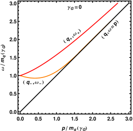
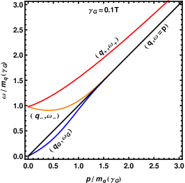
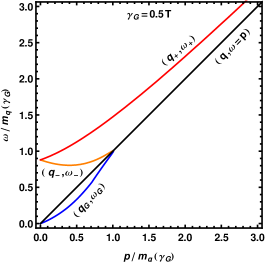
Figure 1: Plot of the dispersion relations for different values of $\gamma_{G}$. In the parenthesis, the first one represents a collective excitation mode whereas the second one is the corresponding energy of that mode.

Solving for the zeros of $D_{\pm}^{-1}(P,\gamma_{G})$ gives the dispersion relations for the collective excitations in the medium. In Fig. 1 we show the resulting dispersion relations for three different values of the Gribov parameter $\gamma_{G}$. In absence of the Gribov term (i.e, $\gamma_{G}=0$), there are two massive modes corresponding to a normal quark mode $q_{+}$ with energy $\omega_{+}$ and a long wavelength plasmino mode $q_{-}$ with energy $\omega_{-}$ that quickly approaches free massless propagation in the high-momentum limit. These two modes are similar to those found in the HTL approximation yuan . With the inclusion of the Gribov term, there is a massless mode $q_{G}$ with energy $\omega_{G}$, in addition to the two massive modes, $q_{+}$ and $q_{-}$ nansu1 . The extra mode $q_{G}$ is due to the presence of the magnetic screening scale. This new massless mode is lightlike at large momenta. In this context, we note that in Ref. pc3 , such an extra massive mode with significant spectral width was observed near $T_{c}$ in presence of dimension-four gluon condensates pc3 in addition to the usual propagating quark and plasmino modes. The existence of this extra mode could affect lattice extractions of the dilepton rate since even the most recent LQCD results kitazawa1 ; kitazawa2 assumed that there were only two poles (a quark mode and a plasmino mode) inspired by the HTL approximation.

In HTL approximation ($\gamma_{G}=0$) the propagator contains a discontinuity in complex plane stemming from the logarithmic terms in (13) due to spacelike momentum $\omega^{2}<p^{2}$. Apart from two collective excitations originating from the in-medium dispersion as discussed above, there is also a Landau cut contribution in the spectral representation of the propagator due to the discontinuity in spacelike momentum. On the other hand, for $\gamma_{G}\neq 0$ the individual terms in (13) possess discontinuities at spacelike momentum but canceled out when all terms are summed owing the fact that the poles come in complex-conjugate pairs. As a result, there is no discontinuity in the complex plane. This results in disappearance of the Landau cut contribution in the spectral representation of the propagator in spacelike domain. It appears as if the Landau cut contribution in spacelike domain for $\gamma_{G}=0$ is replaced by massless spacelike dispersive mode in presence of magnetic scale ($\gamma_{G}\neq 0$). So the spectral function corresponding to the propagator $D_{\pm}^{-1}$ for $\gamma_{G}\neq 0$ has only pole contributions. As a result, one has

$$\rho_{\pm}^{G}(\omega,p)=\frac{\omega^{2}-p^{2}}{2m_{q}^{2}(\gamma_{G})}\left[\delta(\omega\mp\omega_{+})+\delta(\omega\pm\omega_{-})+\delta(\omega\pm\omega_{G})\right],$$ (14)

where $D_{+}$ has poles at $\omega_{+}$, $-\omega_{-}$, and $-\omega_{G}$ and $D_{-}$ has poles at $\omega_{-}$, $-\omega_{+}$, and $\omega_{G}$ with a prefactor, $(\omega^{2}-p^{2})/2m_{q}^{2}(\gamma_{G})$, as the residue.

At this point we would like to mention that the non-perturbative quark spectral function obtained using the quark propagator analyzed in the quenched LQCD calculations of Refs. kitazawa1 ; kitazawa2 ; kim and utilizing gluon condensates in Refs. schaefer1 ; schaefer2 ; schaefer3 ; peshier ; pc3 also forbids a Landau cut contribution since the effective quark propagators in these calculations do not contain any discontinuities. This stems from the fact that the quark self-energies in Refs. schaefer1 ; schaefer2 ; schaefer3 ; peshier ; pc3 do not have any imaginary parts whereas in Refs. kitazawa1 ; kitazawa2 ; kim an ansatz of two quasiparticles was employed for spectral function based on the LQCD quark propagator analyzed in quenched approximation. The spectral function obtained with the Gribov action (14) also possesses only pole contributions but no Landau cut. As a result, this approach completely removes the quasigluons responsible for the Landau cut that should be present in a high-temperature quark-gluon plasma. This is similar to findings in other nonperturbative approaches kitazawa1 ; kitazawa2 ; kim ; schaefer1 ; schaefer2 ; schaefer3 ; peshier . We will return to the consequences of the absence of Landau cut in the results and conclusions sections.

Returning to the problem at hand, the spectral density in (14) at vanishing three momentum ($p\equiv|\vec{p}|=0$) contains three delta function singularities corresponding to the two massive modes and one new massless Gribov mode. To proceed, one needs the vertex functions in presence of the Gribov term. These can be determined by explicitly computing the hard-loop limit of the vertex function using the Gribov propagator. One can verify, after the fact, that the resulting effective quark-gluon vertex function satisfies the necessary Slavnov-Taylor (ST) identity

$$(P_{1}-P_{2})_{\mu}\Gamma^{\mu}(P_{1},P_{2})=S^{-1}(P_{1})-S^{-1}(P_{2})\ .$$ (15)

The temporal and spatial parts of the modified effective quark-gluon vertex can be written as

$$\Gamma^{0} = a_{G}~{}\gamma^{0}+b_{G}~{}\bf{\gamma}\cdot\hat{\bf{p}},$$

$$\Gamma^{i} = c_{G}~{}\gamma^{i}+b_{G}~{}\hat{p}^{i}\gamma_{0}+d_{G}~{}\hat{p}^{i}\left(\bf{\gamma}\cdot\hat{\bf{p}}\right),$$ (16)

where the coefficients are given by

$$a_{G} = 1-\frac{2g^{2}C_{F}}{(2\pi)^{2}}\sum_{\pm}\int dk\,k\,\tilde{n}_{\pm}(k,\gamma_{G})\frac{1}{\omega_{1}-\omega_{2}}\left[\delta Q_{01}^{\pm}+\delta Q_{02}^{\pm}\right],$$

$$b_{G} = -\frac{2g^{2}C_{F}}{(2\pi)^{2}}\sum_{\pm}\int dk\,k\,\tilde{n}_{\pm}(k,\gamma_{G})\frac{1}{\omega_{1}-\omega_{2}}\left[\delta Q_{11}^{\pm}+\delta Q_{12}^{\pm}\right],$$

$$c_{G} = 1+\frac{2g^{2}C_{F}}{(2\pi)^{2}}\sum_{\pm}\int dk\,k\,\tilde{n}_{\pm}(k,\gamma_{G})\frac{1}{3(\omega_{1}-\omega_{2})}\left[\delta Q_{01}^{\pm}+\delta Q_{02}^{\pm}-\delta Q_{21}^{\pm}-\delta Q_{22}^{\pm}\right],$$

$$d_{G} = \frac{2g^{2}C_{F}}{(2\pi)^{2}}\sum_{\pm}\int dk\,k\,\tilde{n}_{\pm}(k,\gamma_{G})\frac{1}{\omega_{1}-\omega_{2}}\left[\delta Q_{21}^{\pm}+\delta Q_{22}^{\pm}\right],$$

with

$$\delta Q_{n1}^{\pm} = Q_{n}(\tilde{\omega}_{11}^{\pm},p)-Q_{n}(\tilde{\omega}_{21}^{\pm},p){\rm{~{}for~{}}}n=0,1,2\,\,,$$

$$\omega_{m1}^{\pm} = E_{\pm}^{0}(\omega_{m}+k-E_{\pm}^{0})/k{\rm{~{}for~{}}}m=1,2\,\,,$$

$$\omega_{m2}^{\pm} = E_{\pm}^{0}(\omega_{m}-k+E_{\pm}^{0})/k{\rm{~{}for~{}}}m=1,2\,\,.$$

Similarly, the four-point function can be obtained by computing the necessary diagrams in the hard-loop limit and it satisfies the following generalized ST identity

$$P_{\mu}\Gamma^{\mu\nu}(-P_{1},P_{1};-P_{2},P_{2})=\Gamma^{\nu}(P_{1}-P_{2},-P_{1};P_{2})-\Gamma^{\nu}(-P_{1}-P_{2},P_{1};P_{2})\ .$$ (17)

III One-loop dilepton production with the Gribov action

The dilepton production rate for a dilepton with energy $\omega$ and three-momentum ${\vec{q}}$ is related to the discontinuity of the photon self energy $\Pi^{\mu\nu}(Q)$ as larry

$$\frac{dR}{d\omega d^{3}q}=\frac{\alpha}{12\pi^{3}Q^{2}}\frac{1}{e^{\beta\omega}-1}\frac{1}{2\pi i}\,\textmd{Disc}\,\Pi_{\mu}^{\mu}(Q).$$ (18)

At one-loop order, the dilepton production rate is related to the two diagrams shown in Fig. 2, which can be written as

$$\Pi_{\mu}^{\mu}(Q) = \frac{5}{3}e^{2}\sum_{p_{0}}\int\frac{d^{3}p}{(2\pi)^{3}}\biggl{\{}\textmd{Tr}\biggl{[}S(P)~{}\Gamma_{\mu}(K,Q,-P)~{}S(K)~{}\Gamma_{\mu}(-K,-Q,P)\biggr{]}$$ (19)

$$\hskip 142.26378pt+\;\textmd{Tr}\biggl{[}S(P)~{}\Gamma_{\mu}^{\mu}(-P,P;-Q,Q)\biggr{]}\biggr{\}},$$

where $K=P-Q$. The second term in (19) is due to the tadpole diagram shown in Fig. 2 which, in the end, does not contribute since $\Gamma_{\mu}^{\mu}=0$. However, the tadpole diagram is essential to satisfy the transversality condition, $Q_{\mu}\Pi^{\mu\nu}(Q)=0$ and thus gauge invariance and charge conservation in the system.

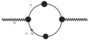
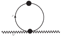
Figure 2: The self-energy (left) and tadpole (right) diagrams in one loop order.

Using the $n$-point functions computed in sec. II and performing traces, one obtains

$$\Pi_{\mu}^{\mu}(\vec{q}=0) = \frac{10}{3}e^{2}T\sum_{p_{0}}\int\frac{d^{3}p}{(2\pi)^{3}}$$ (20)

$$\times\Biggl{[}\left\{\frac{(a_{G}+b_{G})^{2}}{D_{+}(\omega_{1},p,\gamma_{G})D_{-}(\omega_{2},p,\gamma_{G})}+\frac{(a_{G}-b_{G})^{2}}{D_{-}(\omega_{1},p,\gamma_{G})D_{+}(\omega_{2},p,\gamma_{G})}\right\}$$

$$-\left\{\frac{(c_{G}+b_{G}+d_{G})^{2}}{D_{+}(\omega_{1},p,\gamma_{G})D_{-}(\omega_{2},p,\gamma_{G})}+\frac{(c_{G}-b_{G}+d_{G})^{2}}{D_{-}(\omega_{1},p,\gamma_{G})D_{+}(\omega_{2},p,\gamma_{G})}\right\}$$

$$-2c_{G}^{2}\left\{\frac{1}{D_{+}(\omega_{1},p,\gamma_{G})D_{+}(\omega_{2},p,\gamma_{G})}+\frac{1}{D_{-}(\omega_{1},p,\gamma_{G})D_{-}(\omega_{2},p,\gamma_{G})}\right\}\Biggr{]}.$$

The discontinuity can be obtained by Braaten-Pisarski-Yuan (BPY) prescription yuan

$$\textmd{Disc~{}}T\sum_{p_{0}}f_{1}(p_{0})f_{2}(q_{0}-p_{0}) = 2\pi i(1-e^{\beta\omega})\int d\omega_{1}\int d\omega_{2}~{}n_{F}(\omega_{1})n_{F}(\omega_{2})$$ (21)

$$\times\ \delta(\omega-\omega_{1}-\omega_{2})\ \rho_{1}(\omega_{1})\rho_{2}(\omega_{2}),$$

which, after some work, allows one to determine the dilepton rate at zero three momentum

$$\frac{dR}{d\omega d^{3}q}({\vec{q}}=0) = \frac{10\alpha^{2}}{9\pi^{4}}\frac{1}{\omega^{2}}\int\limits_{0}^{\infty}p^{2}dp\int\limits_{-\infty}^{\infty}d\omega_{1}\int\limits_{-\infty}^{\infty}d\omega_{2}n_{F}(\omega_{1})n_{F}(\omega_{2})\delta(\omega-\omega_{1}-\omega_{2})$$ (22)

$$\Bigg{[}4\left(1-\frac{\omega_{1}^{2}-\omega_{2}^{2}}{2p\,\omega}\right)^{2}\rho_{+}^{G}(\omega_{1},p)\rho_{-}^{G}(\omega_{2},p)$$

$$+\left(1+\frac{\omega_{1}^{2}+\omega_{2}^{2}-2p^{2}-2m_{q}^{2}(\gamma_{G})}{2p\,\omega}\right)^{2}\rho_{+}^{G}(\omega_{1},p)\rho_{+}^{G}(\omega_{2},p)$$

$$+\left(1-\frac{\omega_{1}^{2}+\omega_{2}^{2}-2p^{2}-2m_{q}^{2}(\gamma_{G})}{2p\,\omega}\right)^{2}\rho_{-}^{G}(\omega_{1},p)\rho_{-}^{G}(\omega_{2},p)\Bigg{]}.$$

Using (14) and considering all physically allowed processes by the in-medium dispersion, the total contribution can be expressed as

$$\frac{dR}{d\omega d^{3}q}\Big{|}^{pp}({\vec{q}}=0) = \frac{10\alpha^{2}}{9\pi^{4}}\frac{1}{\omega^{2}}\int\limits_{0}^{\infty}p^{2}\,dp\times$$ (23)

$$\Biggl{[}\delta(\omega-2\omega_{+})\ n_{F}^{2}(\omega_{+})\left(\frac{\omega_{+}^{2}-p^{2}}{2m_{q}^{2}(\gamma_{G})}\right)^{2}\left\{1+\frac{\omega_{+}^{2}-p^{2}-m_{q}^{2}(\gamma_{G})}{p~{}\omega}\right\}^{2}$$

$$+~{}\delta(\omega-2\omega_{-})\ n_{F}^{2}(\omega_{-})\left(\frac{\omega_{-}^{2}-p^{2}}{2m_{q}^{2}(\gamma_{G})}\right)^{2}\left\{1-\frac{\omega_{-}^{2}-p^{2}-m_{q}^{2}(\gamma_{G})}{p~{}\omega}\right\}^{2}$$

$$+~{}\delta(\omega-2\omega_{G})\ n_{F}^{2}(\omega_{G})\left(\frac{\omega_{G}^{2}-p^{2}}{2m_{q}^{2}(\gamma_{G})}\right)^{2}\left\{1-\frac{\omega_{G}^{2}-p^{2}-m_{q}^{2}(\gamma_{G})}{p~{}\omega}\right\}^{2}$$

$$+4\ \delta(\omega-\omega_{+}-\omega_{-})\ n_{F}(\omega_{+})\ n_{F}(\omega_{-})\left(\frac{\omega_{+}^{2}-p^{2}}{2m_{q}^{2}(\gamma_{G})}\right)\left(\frac{\omega_{-}^{2}-p^{2}}{2m_{q}^{2}(\gamma_{G})}\right)$$

$$\times\left\{1-\frac{\omega_{+}^{2}-\omega_{-}^{2}}{2p\,\omega}\right\}^{2}$$

$$+\delta(\omega-\omega_{+}+\omega_{-})\ n_{F}(\omega_{+})n_{F}(-\omega_{-})\left(\frac{\omega_{+}^{2}-p^{2}}{2m_{q}^{2}(\gamma_{G})}\right)\left(\frac{\omega_{-}^{2}-p^{2}}{2m_{q}^{2}(\gamma_{G})}\right)$$

$$\times\left\{1+\frac{\omega_{+}^{2}+\omega_{-}^{2}-2p^{2}-2m_{q}^{2}(\gamma_{G})}{2p\,\omega}\right\}^{2}~{}\Biggr{]}.$$

Inspecting the arguments of the various energy conserving $\delta$-functions in (23) one can understand the physical processes originating from the poles of the propagator. The first three terms in (23) correspond to the annihilation processes of $q_{+}{\bar{q}}_{+}\rightarrow\gamma^{*}$, $q_{-}{\bar{q}}_{-}\rightarrow\gamma^{*}$, and $q_{G}{\bar{q}}_{G}\rightarrow\gamma^{*}$, respectively. The fourth term corresponds to the annihilation of $q_{+}{\bar{q}}_{-}\rightarrow\gamma^{*}$. On the other hand, the fifth term corresponds to a process, $q_{+}\rightarrow q_{-}\gamma*$, where a $q_{+}$ mode makes a transition to a $q_{-}$ mode along with a virtual photon. These processes involve soft quark modes ($q_{+},\,q_{-}$, and $q_{G}$ and their antiparticles) which originate by cutting the self-energy diagram in Fig. 2 through the internal lines without a “blob”. The virtual photon, $\gamma^{*}$, in all these five processes decays to lepton pair and can be visualized from the dispersion plot as displayed in the Fig. 3. The momentum integration in Eq. (23) can be performed using the standard delta function identity

$$\delta(f(x)) = \sum_{i}\frac{\delta(x-x_{i})}{\mid\!f^{\prime}(x)\!\mid_{x=x_{i}}},$$ (24)

where $x_{i}$ are the solutions of $f(x_{i})=0$.

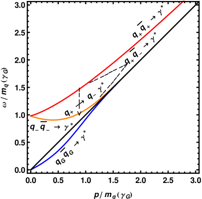
Figure 3: Various dilepton processes which originate from the in-medium dispersion with the Gribov term.

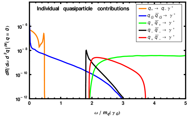
Figure 4: The dilepton production rates corresponding to quasiparticle processes in Fig. 3.

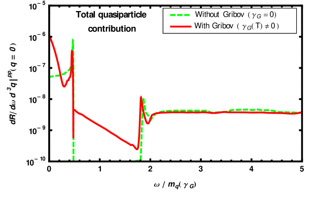
Figure 5: Comparison of dilepton production rates involving various quasiparticle modes with and without inclusion of $\gamma_{G}$.

The contribution of various individual processes to the dilepton production rate in presence of the Gribov term are displayed in the Fig. 4. Note that in this figure and in subsequent figures showing the dilepton rate, the vertical axis shows the dimensional late dilepton rate $dR/d^{4}p=dN/d^{4}xd^{4}p$ and the horizontal axis is scaled by the thermal quark mass as to make it dimensionless. In Fig. 4 we see that the transition process, $q_{+}\rightarrow q_{-}\gamma*$, begins at the energy $\omega=0$ and ends up with a van-Hove peak  where all of the transitions from $q_{+}$ branch are directed towards the minimum of the $q_{-}$ branch. The annihilation process involving the massless spacelike Gribov modes, $q_{G}{\bar{q}}_{G}\rightarrow\gamma^{*}$, also starts at $\omega=0$ and falls-off very quickly. The annihilation of the two plasmino modes, $q_{-}{\bar{q}}_{-}\rightarrow\gamma^{*}$, opens up with again a van-Hove peak at $\omega=2\times$ the minimum energy of the plasmino mode. The contribution of this process decreases exponentially. At $\omega=2m_{q}(\gamma_{G})$, the annihilation processes involving usual quark modes, $q_{+}{\bar{q}}_{+}\rightarrow\gamma^{*}$, and that of a quark and a plasmino mode, $q_{+}{\bar{q}}_{-}\rightarrow\gamma^{*}$, begin. However, the former one ($q_{+}{\bar{q}}_{+}\rightarrow\gamma^{*}$) grows with the energy and would converge to the usual Born rate (leading order perturbative rate) born at high mass whereas the later one ($q_{+}{\bar{q}}_{-}\rightarrow\gamma^{*}$) initially grows at a very fast rate, but then decreases slowly and finally drops very quickly. The behavior of the latter process can easily be understood from the dispersion properties of quark and plasmino mode. Summing up, the total contribution of all theses five processes is displayed in Fig. 5. This is compared with the similar dispersive contribution when $\gamma_{G}=0$ yuan , comprising processes $q_{+}\rightarrow q_{-}\gamma*$, $q_{+}{\bar{q}}_{+}\rightarrow\gamma^{*}$, $q_{-}{\bar{q}}_{-}\rightarrow\gamma^{*}$ and $q_{+}{\bar{q}}_{-}\rightarrow\gamma^{*}$. We note that when $\gamma_{G}=0$, the dilepton rate contains both van-Hove peaks and an energy gap yuan . In presence of the Gribov term ($\gamma_{G}\neq 0$), the van-Hove peaks remain, but the energy gap disappears due to the annihilation of new massless Gribov modes, $q_{G}{\bar{q}}_{G}\rightarrow\gamma^{*}$.

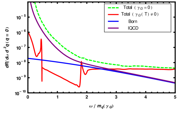
Figure 6: Comparison of various dilepton production rates from the deconfined matter.

In Fig. 6 we compare the rates obtained using various approximations: leading-order perturbative (Born) rate born , quenched LQCD rate ding ; laermann , and with and without the Gribov term. The non-perturbative rate with the Gribov term shows important structures compared to the Born rate at low energies. But when compared to the total HTLpt rate  it is suppressed in the low mass region due to the absence of Landau cut contribution for $\gamma_{G}\neq 0$. It seems as if the higher order Landau cut contribution due to spacelike momenta for $\gamma_{G}=0$ is replaced by the soft process involving spacelike Gribov modes in the collective excitations for $\gamma_{G}\neq 0$. We also note that the dilepton rate kim using the spectral function constructed with two pole ansatz by analyzing LQCD propagator in quenched approximation kitazawa1 ; kitazawa2 shows similar structure as found here for $\gamma_{G}\neq 0$. On the other hand, such structure at low mass is also expected in the direct computation of dilepton rate from LQCD in quenched approximation ding ; laermann . However, a smooth variation of the rate was found at low mass. The computation of dilepton rate in LQCD involves various intricacies and uncertainties. This is because, as noted in sec. I, the spectral function in continuous time is obtained from the correlator in finite set of discrete Euclidean time using a probabilistic MEM method mem1 ; mem2 ; mem3 with a somewhat ad hoc continuous ansatz for the spectral function at low energy and also fundamental difficulties in performing the necessary analytic continuation in LQCD. Until LQCD overcomes the uncertainties and difficulties in the computation of the vector spectral function, one needs to depend, at this juncture, on the prediction of the effective approaches for dilepton rate at low mass in particular. We further note that at high-energies the rate for both $\gamma_{G}=0$ and $\gamma_{G}\neq 0$ is higher than the lattice data and Born rate. This is a consequence of using the HTL self-energy also at high-energies/momentum where the soft-scale approximation breaks down. Nevertheless, the low mass rate obtained here by employing the non-perturbative magnetic scale ($\gamma_{G}\neq 0$) in addition to the electric scale allows for a model-based inclusion of the effect of confinement and the result has a somewhat rich structure at low energy compared to that obtained using only the electric scale ($\gamma_{G}=0$) as well in LQCD.

We make some general comments concerning the dilepton rate below. If one looks at the dispersion plots in Fig. 1 for $\gamma_{G}=0$, then one finds that $\omega_{-}$ falls off exponentially and approaches light cone, whereas $\omega_{+}$ does not follow fall off exponentially to light cone, but instead behaves as $[p+m^{2}_{q}(T)/p]$ for large $p$. On the other hand, in the presence of $\gamma_{G}\neq 0$ both $\omega_{-}$ and $\omega_{G}$ approach the light cone very quickly, but again $\omega_{+}$ has a similar asymptotic behavior as before. This feature of $\omega_{+}$ makes the dilepton rate at large $\omega$ in Fig. 6 saturate for both $\gamma_{G}=0$ and $\gamma_{G}\neq 0$, because the dominant contribution comes from the annihilation of two $\omega_{+}$ as discussed in Fig. 4. In general, the total dilepton rate in Fig. 6, behaves as $\sim\exp(-\omega/T)$ for $\gamma_{G}(T)=0$ due to the Landau damping contribution coming from the quasigluons in a hot and dense medium. As the Landau cut contribution is missing in the $\gamma_{G}(T)\neq 0$ case, one finds a leveling off at low $\omega$. In other words, since the Landau damping contribution is absent for $\gamma_{G}(T)\neq 0$, the rate approaches that of the pole-pole contribution for $\gamma_{G}=0$ as shown in Fig. 5, except in the mass gap region. We further note that the LQCD rate ding matches with Born rate at large $\omega$ simply because a free spectral function has been assumed for large $\omega$. On the other hand the LQCD spectral function ding at low $\omega$ is sensitive to the prior assumptions and, in such a case, the spectral function extracted using a MEM mem1 ; mem2 ; mem3 analyses should be interpreted carefully with a proper error analysis mem1 . Since the MEM analyses is sensitive to the prior assumption, but is not very sensitive to the structure of the spectral function at small $\omega$, the error is expected to be significant at small $\omega$. The existence of fine structure such as van Hove singularities at small $\omega$ cannot be excluded based on the LQCD rate ding at this moment in time.

IV One-loop quark number susceptibility with the Gribov action

We now turn to the computation of the quark number susceptibility (QNS) including the Gribov term. The QNS can be interpreted as the response of the conserved quark number density, $n$ with infinitesimal variation in the quark chemical potentials $\mu+\delta\mu$. In QCD thermodynamics it is defined as the second order derivative of pressure ${\cal P}$ with respect to quark chemical potential, $\mu$. But again, using the fluctuation-dissipation (FD) theorem, the QNS for a given quark flavor can also be defined from the time-time component of the current-current correlator in the vector channel purnendu1 ; purnendu3 ; forster ; kunihiro . The QNS is in general expressed as

$$\chi_{q}(T) = \!\!\left.\frac{\partial n}{\partial\mu}\right|_{\mu\rightarrow 0}\!\!\!=\!\!\!\left.\frac{\partial^{2}{\cal P}}{\partial^{2}\mu}\right|_{\mu\rightarrow 0}\!\!\!=\int d^{4}x\langle J_{0}(0,{\vec{x}})J_{0}(0,{\vec{0}})\rangle$$ (25)

$$= \beta\int\limits_{-\infty}^{\infty}\frac{d\omega}{2\pi}\frac{-2}{1-e^{-\beta\omega}}~{}\textmd{Im}~{}\Pi_{00}(\omega,{\vec{0}}),$$

where $J_{0}$ is the temporal component of the vector current and $\Pi_{00}$ is the time-time component of the vector correlator or self-energy with external four-momenta $Q\equiv(\omega,\vec{q})$. The above relation in (25) is known as the thermodynamic sum rule forster ; kunihiro where the thermodynamic derivative with respect to the external source, $\mu$ is related to the time-time component of static correlation function in the vector channel.

In order to compute the QNS we need to calculate the imaginary part of the temporal component of the two one-loop diagrams given in Fig. 2. The contribution of the self energy diagram is

$$\Pi^{s}_{00}(Q) = N_{f}N_{c}T\sum_{p_{0}}\int\frac{d^{3}p}{(2\pi)^{3}}\textmd{Tr}\left[S(P)~{}\Gamma^{0}(K,Q,-P)~{}S(K)~{}\Gamma^{0}(-K,-Q,P)\right],$$ (26)

where $K=P-Q$. After performing the traces of the self energy diagram, one obtains

$$\Pi^{s}_{00}(\vec{q}=0) = 2N_{f}N_{c}T\sum_{p_{0}}\int\!\!\!\frac{d^{3}p}{(2\pi)^{3}}\left[\frac{(a_{G}+b_{G})^{2}}{D_{+}(\omega_{1},p,\gamma_{G})D_{-}(\omega_{2},p,\gamma_{G})}\right.$$ (27)

$$\hskip 93.89418pt+\left.\frac{(a_{G}-b_{G})^{2}}{D_{-}(\omega_{1},p,\gamma_{G})D_{+}(\omega_{2},p,\gamma_{G})}\right],$$

where

$$a_{G}+b_{G} = 1-\frac{2g^{2}C_{F}}{(2\pi)^{2}}\sum_{\pm}\int dkk\tilde{n}_{\pm}(k,\gamma_{G})\frac{1}{\omega}$$ (28)

$$\times\Bigl{[}Q_{0}(\tilde{\omega}_{11}^{\pm},p)+Q_{1}(\tilde{\omega}_{11}^{\pm},p)+Q_{0}(\tilde{\omega}_{21}^{\pm},p)-Q_{1}(\tilde{\omega}_{21}^{\pm},p)$$

$$+Q_{0}(\tilde{\omega}_{12}^{\pm},p)+Q_{1}(\tilde{\omega}_{12}^{\pm},p)+Q_{0}(\tilde{\omega}_{22}^{\pm},p)-Q_{1}(\tilde{\omega}_{22}^{\pm},p)\Bigr{]}$$

$$= 1+\frac{1}{\omega}\left[D_{+}(\omega_{1},p,\gamma_{G})+D_{-}(\omega_{2},p,\gamma_{G})-\omega_{1}-\omega_{2}\right]$$

$$= 1-\frac{\omega_{1}+\omega_{2}}{\omega}+\frac{D_{+}(\omega_{1},p,\gamma_{G})+D_{-}(\omega_{2},p,\gamma_{G})}{\omega},$$

and

$$a_{G}-b_{G} = 1-\frac{2g^{2}C_{F}}{(2\pi)^{2}}\sum_{\pm}\int dkk\tilde{n}_{\pm}(k,\gamma_{G})\frac{1}{\omega}$$ (29)

$$\times\Bigl{[}Q_{0}(\tilde{\omega}_{11}^{\pm},p)-Q_{1}(\tilde{\omega}_{11}^{\pm},p)+Q_{0}(\tilde{\omega}_{21}^{\pm},p)+Q_{1}(\tilde{\omega}_{21}^{\pm},p)$$

$$+Q_{0}(\tilde{\omega}_{12}^{\pm},p)-Q_{1}(\tilde{\omega}_{12}^{\pm},p)+Q_{0}(\tilde{\omega}_{22}^{\pm},p)+Q_{1}(\tilde{\omega}_{22}^{\pm},p)\Bigr{]}$$

$$= 1+\frac{1}{\omega}\left[D_{-}(\omega_{1},p,\gamma_{G})+D_{+}(\omega_{2},p,\gamma_{G})-\omega_{1}-\omega_{2}\right]$$

$$= 1-\frac{\omega_{1}+\omega_{2}}{\omega}+\frac{D_{-}(\omega_{1},p,\gamma_{G})+D_{+}(\omega_{2},p,\gamma_{G})}{\omega},$$

where $D_{\mp}(\omega,p,\gamma_{G})$ were defined in Eq. (13). We write only those terms of Eq. (27) which contain discontinuities

$$\frac{(a_{G}+b_{G})^{2}}{D_{+}(\omega_{1},p,\gamma_{G})D_{-}(\omega_{2},p,\gamma_{G})} = \frac{(1-\frac{\omega_{1}+\omega_{2}}{\omega})^{2}}{D_{+}(\omega_{1},p,\gamma_{G})D_{-}(\omega_{2},p,\gamma_{G})}$$

$$\hskip 14.22636pt+\frac{1}{\omega^{2}}\left\{\frac{D_{+}(\omega_{1},p,\gamma_{G})}{D_{-}(\omega_{2},p,\gamma_{G})}+\frac{D_{-}(\omega_{2},p,\gamma_{G})}{D_{+}(\omega_{1},p,\gamma_{G})}\right\},$$

$$\frac{(a_{G}-b_{G})^{2}}{D_{-}(\omega_{1},p,\gamma_{G})D_{+}(\omega_{2},p,\gamma_{G})} = \frac{(1-\frac{\omega_{1}+\omega_{2}}{\omega})^{2}}{D_{-}(\omega_{1},p,\gamma_{G})D_{+}(\omega_{2},p,\gamma_{G})}$$ (30)

$$\hskip 14.22636pt+\frac{1}{\omega^{2}}\left\{\frac{D_{-}(\omega_{1},p,\gamma_{G})}{D_{+}(\omega_{2},p,\gamma_{G})}+\frac{D_{+}(\omega_{2},p,\gamma_{G})}{D_{-}(\omega_{1},p,\gamma_{G})}\right\}.$$

Calculating the discontinuity using the BPY prescription given in Eq. (21), one can write the imaginary part of Eq. (27) as

$$\textmd{Im}~{}\Pi^{s}_{00} = 4N_{c}N_{f}\pi(1-e^{\beta\omega})\int\frac{d^{3}p}{(2\pi)^{3}}\int d\omega_{1}\int d\omega_{2}~{}\delta(\omega-\omega_{1}-\omega_{2})n_{F}(\omega_{1})n_{F}(\omega_{2})$$ (31)

$$\times\Bigl{[}\left(1-\frac{\omega_{1}+\omega_{2}}{\omega}\right)^{2}\rho_{+}^{G}(\omega_{1},p)\rho_{-}^{G}(\omega_{2},p)+\frac{C_{1}\rho_{+}^{G}(\omega_{2},p)+C_{2}\rho_{-}^{G}(\omega_{2},p)}{\omega^{2}}\Bigr{]},$$

with

$$C_{1} = \textmd{Im}~{}D_{-}(\omega_{1},p)=0,$$

$$C_{2} = \textmd{Im}~{}D_{+}(\omega_{1},p)=0.$$ (32)

The tadpole part of Fig. 2 can now be written as

$$\Pi^{t}_{00}(Q) = N_{f}N_{c}T\sum_{p_{0}}\int\frac{d^{3}p}{(2\pi)^{3}}\textmd{Tr}\biggl{[}S(P)~{}\Gamma_{00}(-P,P;-Q,Q)\biggr{]}.$$ (33)

The four-point function $\Gamma_{00}$ at zero three-momentum can be obtained using Eq. (17) giving

$$\Gamma^{00} = -(e_{G}\gamma^{0}+f_{G}~{}\hat{p}\cdot\vec{\gamma}),$$ (34)

$$e_{G} = \frac{2g^{2}c_{F}}{(2\pi)^{2}}\sum_{\pm}\int dkk\tilde{n}_{\pm}(k,\gamma_{G})\frac{1}{(\omega_{1}-\omega_{2})}\left[\delta Q_{01}^{\pm}+\delta Q_{02}^{\pm}+\delta Q_{01}^{\pm\prime}+\delta Q_{02}^{\pm\prime}\right],$$

$$f_{G} = \frac{2g^{2}c_{F}}{(2\pi)^{2}}\sum_{\pm}\int dkk\tilde{n}_{\pm}(k,\gamma_{G})\frac{1}{(\omega_{1}-\omega_{2})}\left[\delta Q_{11}^{\pm}+\delta Q_{12}^{\pm}+\delta Q_{11}^{\pm\prime}+\delta Q_{12}^{\pm\prime}\right],$$

where

$$\delta Q_{n1}^{\pm\prime} = Q_{n}(\tilde{\omega}_{11}^{\pm},p)-Q_{n}(\tilde{\omega}_{21}^{\pm\prime},p){\rm{~{}for~{}}}n=0,1,2\,\,,$$

$$\tilde{\omega}_{21}^{\pm\prime} = E_{\pm}^{0}(\omega_{2}^{\prime}+k-E_{\pm}^{0})/k\,,$$

$$\tilde{\omega}_{22}^{\pm\prime} = E_{\pm}^{0}(\omega_{2}^{\prime}-k+E_{\pm}^{0})/k\,,$$

$$\omega_{2}^{\prime} = \omega_{1}+\omega.$$

Proceeding in a similar way as the self-energy diagram, the contribution from the tadpole diagram is

$$\textmd{Im}~{}\Pi_{00}^{t} = -4N_{c}N_{f}\pi(1-e^{\beta\omega})\int\frac{d^{3}p}{(2\pi)^{3}}\int d\omega_{1}\int d\omega_{2}~{}\delta(\omega-\omega_{1}-\omega_{2})\frac{n_{F}(\omega_{1})n_{F}(\omega_{2})}{\omega^{2}}$$ (35)

$$\times\Bigl{[}C_{1}\rho_{+}^{G}(\omega_{2},p)+C_{2}\rho_{-}^{G}(\omega_{2},p)\Bigr{]}=0.$$

The total imaginary contribution of the temporal part shown in Fig. 2 can now be written as

$$\textmd{Im}~{}\Pi_{00} = \textmd{Im}~{}\Pi^{s}_{00}+\textmd{Im}~{}\Pi^{t}_{00}$$ (36)

$$= 4N_{c}N_{f}\pi(1-e^{\beta\omega})\int\frac{d^{3}p}{(2\pi)^{3}}\int d\omega_{1}\int d\omega_{2}~{}\delta(\omega-\omega_{1}-\omega_{2})n_{F}(\omega_{1})n_{F}(\omega_{2})$$

$$\times\Bigl{[}\left(1-\frac{\omega_{1}+\omega_{2}}{\omega}\right)^{2}\rho_{+}^{G}(\omega_{1},p)\rho_{-}^{G}(\omega_{2},p)\Bigr{]}.$$

It is clear from (31) and (35) that the tadpole contribution in (35) exactly cancels with the second term of (31) even if $C_{1}$ and $C_{2}$ are finite, e.g., for the HTL case ($\gamma_{G}=0$) purnendu1 ; purnendu3 . At finite $\gamma_{G}$, the form of the sum of self-energy and tadpole diagrams remains the same, even though the individual contribution are modified.

Putting this in the expression for the QNS in Eq. (25), we obtain

$$\chi_{q}(T) = 4N_{c}N_{f}\beta\int\frac{d^{3}p}{(2\pi)^{3}}\int\limits_{-\infty}^{\infty}d\omega\int d\omega_{1}\int d\omega_{2}~{}\delta(\omega-\omega_{1}-\omega_{2})n_{F}(\omega_{1})n_{F}(\omega_{2})$$ (37)

$$\hskip 28.45274pt\times\Big{[}\left(1-\frac{\omega_{1}+\omega_{2}}{\omega}\right)^{2}\rho_{+}^{G}(\omega_{1},p)\rho_{-}^{G}(\omega_{2},p)\Big{]}$$

$$= 4N_{c}N_{f}\beta\int\frac{d^{3}p}{(2\pi)^{3}}\Bigl{[}\left(\frac{\omega_{+}^{2}-p^{2}}{2m_{q}^{2}(\gamma_{G})}\right)^{2}n_{F}(\omega_{+})n_{F}(-\omega_{+})$$

$$+ \left(\frac{\omega_{-}^{2}-p^{2}}{2m_{q}^{2}(\gamma_{G})}\right)^{2}n_{F}(\omega_{-})n_{F}(-\omega_{-})+\left(\frac{\omega_{G}^{2}-p^{2}}{2m_{q}^{2}(\gamma_{G})}\right)^{2}n_{F}(\omega_{G})n_{F}(-\omega_{G})\Bigr{]}$$

$$= \chi_{q}^{\rm{pp}}(T).$$

where we represent the total $\chi_{q}(T)$ as $\chi^{\rm{pp}}_{q}(T)$ since there is only the pole-pole contribution for $\gamma_{G}\neq 0$. However for $\gamma_{G}=0$ there will be pole-cut ($\chi^{\rm{pc}}_{q}(T)$) and cut-cut ($\chi^{\rm{cc}}_{q}(T))$ contribution in addition to pole-pole contribution because the spectral function contains pole part + Landau cut contribution of the quark propagator.

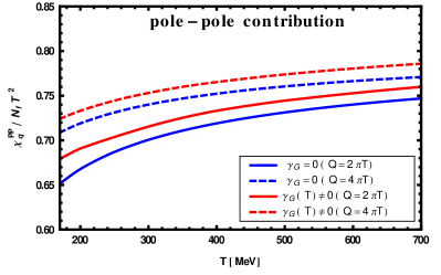
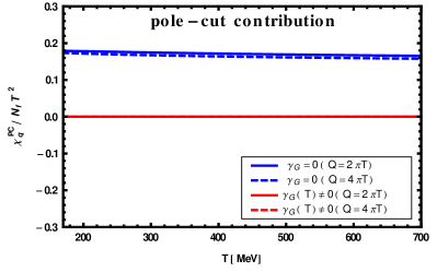
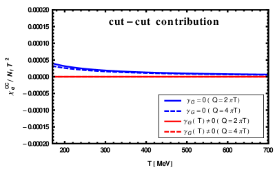
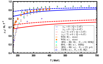
Figure 7: QNS scaled with free values are compared with and without the inclusion of $\gamma_{G}$. In each case a band appears due to the choice of the two renormalization scales as $2\pi T$ and $4\pi T$. The various symbols correspond to LQCD data from various groups labeled as WB borsanyi2 , BNL-BI(B) and BNL-BI(u) bnlb1 ; bnlb2 , and TIFR tifr .

In Fig. 7 we have presented the different contribution of QNS scaled with the corresponding free values with and without the Gribov term. We, at first, note that the running coupling in (3) is a smooth function of $T$ around and below $T_{c}$. We have extended to low temperatures as an extrapolation of our high-temperature result even though our treatment is strictly not valid below $T_{c}$. Now from the first panel of Fig. 7, the pole-pole contribution to the QNS with the Gribov action is increased at low $T$, compared to that in absence of the Gribov term. This improvement at low $T$ is solely due to the presence of the non-perturbative Gribov mode in the collective excitations. However, at high $T$ both contributions become almost same as the Gribov mode disappears. There are no pole-cut (pc) or cut-cut (cc) contribution for $\gamma_{G}(T)\neq 0$, compared to that for $\gamma_{G}=0$. The pc and cc contributions in absence of magnetic scale are displayed in second and third panels. As a result, we find that the QNS in presence of magnetic scale contains only the pp-contribution due to collective excitations originating from the in-medium dispersion whereas, in absence of magnetic scale, the QNS is enhanced due to additional higher order Landau cut (i.e., pole-cut + cut-cut) contribution as shown in the fourth panel. When compared with LQCD data from various groups borsanyi2 ; bnlb1 ; bnlb2 ; tifr , the QNS in presence of magnetic scale lies around $(10-15)\%$ below the LQCD results whereas that in absence of magnetic scale is very close to LQCD data. This is expected due to the additional higher-order Landau cut contribution in absence of magnetic scale as discussed earlier. This also suggests that it is necessary to include higher loop orders in QNS in presence of the magnetic scale, which is beyond scope of this paper. However, we hope to carry out this non-trivial task in near future.

V Conclusions and outlook

In this paper we considered the effect of inclusion of magnetic screening in the context of the Gribov-Zwanziger picture of confinement. In covariant gauge, this was accomplished by adding a masslike parameter, the Gribov parameter, to the bare gluon propagator resulting in the non-propagation of gluonic modes. Following Ref. nansu1 we obtained the resummed quark propagator taking into account the Gribov parameter. A new key feature of the resulting resummed quark propagator is that it contains no discontinuities. In the standard perturbative hard-thermal loop approach there are discontinuities at spacelike momentum associated with Landau damping which seem to be absent in the GZ-HTL approach. Using the resulting quark propagator, we evaluated the spectral function, finding that it only contains poles for $\gamma_{G}\neq 0$. We then used these results to compute (1) the dilepton production rate at vanishing three-momentum and (2) the quark number susceptibility. For the dilepton production rate, we found that, due to the absence of Landau damping for $\gamma_{G}\neq 0$, the rate contains sharp structures, e.g. Van Hove singularities, which don’t seem to be present in the lattice data. That being said, since the lattice calculations used a perturbative ansatz for the spectral function when performing their MEM analysismem1 of the spectral function, it is unclear how changing the underlying prior assumptions about the spectral function would affect the final lattice results. Moreover, the error analsis for spectral function with MEM prescription mem2 has to be done carefully than it was done in LQCD calculation ding . Since the result is sensitive to the prior assumptions, the error seems to become large and as a result no conclusion can be drawn for fine structures at low mass dileptons from the LQCD result. For the quark number susceptibilities, we found that, again due to the absence of Landau damping for $\gamma_{G}\neq 0$, the results do not agree well with available lattice data. This can be contrasted with a standard HTLpt calculation, which seems to describe the lattice data quite well with no free parameters. It is possible that higher-order loop calculations could improve the agreement between the Gribov-scenario results and the lattice data; however, the success of HTLpt compared to lattice data as well as nonperturbative model calculations suggests that at $T\gtrsim$ 200 MeV the electric sector alone provides an accurate description of QGP thermodynamics. Nevertheless, the present HTLpt results poses a serious challenge to the Gribov scenario for only inclusion of magnetic mass effects in the QGP. The absence of quasigluons responsible for the Landau cut makes the results for both dilepton production and quark number susceptibility dramatically different from those in perturbative approaches. We conclude that the results with present GZ action is in conflict with those in perturbative approaches due to the absence of the Landau cut contribution in the non-perturbative quark propagator.

- (1) E.Braaten and R. D. Pisarski, Soft amplitudes in hot gauge theories: A general analysis, Nucl. Phys. B 337, 569-634 (1990).
- (2) E. Braaten and R. D. Pisarski, Resummation and Gauge Invariance of the Gluon Damping Rate in Hot QCD, Phys. Rev. Lett. 64, 1338 (1990).
- (3) E. Braaten and R. D. Pisarski, Simple effective Lagrangian for hard thermal loops, Phys. Rev. D. 45, 1827 (1992).
- (4) J. O. Andersen, E. Braaten, and M. Strickland, Hard thermal loop resummation of the free energy of a hot gluon plasma, Phys. Rev. Lett. 83, 2139 (1999).
- (5) J. O. Andersen, E. Braaten, E. Petitgirard, and M. Strickland, HTL perturbation theory to two loops, Phys. Rev. D. 66, 085016 (2002).
- (6) P. Chakraborty, M. G. Mustafa, and M. H. Thoma, Quark number susceptibility in hard thermal loop approximation, Eur. Phys. J. C. 23, 591 (2002).
- (7) P. Chakraborty, M. G. Mustafa, and M. H. Thoma, Chiral susceptibility in hard thermal loop approximation, Phys. Rev. D. 67, 114004 (2003).
- (8) P. Chakraborty, M. G. Mustafa, and M. H. Thoma, Quark number susceptibility, thermodynamic sum rule, and hard thermal loop approximation, Phys. Rev. D. 68, 085012 (2003).
- (9) J. O. Andersen, E. Petitgirard, and M. Strickland, Two loop HTL thermodynamics with quarks, Phys. Rev. D. 70, 045001 (2004).
- (10) N. Su., J. O. Andersen, and M. Strickland, Gluon Thermodynamics at Intermediate Coupling, Phys. Rev. Lett. 104, 122003 (2010).
- (11) J. O. Andersen, M. Strickland, and N. Su, Three-loop HTL gluon thermodynamics at intermediate coupling, JHEP 1008, 113 (2010).
- (12) N. Haque and M. G. Mustafa, A Modified Hard Thermal Loop Perturbation Theory, arXiv:1007.2076.
- (13) J.O. Andersen, L.E. Leganger, M. Strickland and N. Su, NNLO hard-thermal-loop thermodynamics for QCD, Phys. Lett. B. 696, 468 (2011).
- (14) J. O. Andersen, L. E. Leganger, M. Strickland and N. Su, Three-loop HTL QCD thermodynamics, JHEP 1108, 053 (2011).
- (15) N. Haque, M. G. Mustafa and M. H. Thoma, Conserved Density Fluctuation and Temporal Correlation Function in HTL Perturbation Theory, Phys. Rev. D. 84, 054009 (2011).
- (16) J. O. Andersen, S. Mogliacci, N. Su and A. Vuorinen, Quark number susceptibilities from resummed perturbation theory, Phys. Rev. D 87, 074003 (2013).
- (17) N. Haque, M. G. Mustafa, and M. Strickland, Two-loop HTL pressure at finite temperature and chemical potential, Phys. Rev. D 87, 105007 (2013).
- (18) S. Mogliacci, J. O. Andersen, M. Strickland, N. Su and A. Vuorinen, Equation of State of hot and dense QCD: Resummed perturbation theory confronts lattice data, JHEP 1312, 055 (2013).
- (19) N. Haque, M. G. Mustafa, and M. Strickland, Quark Number Susceptibilities from Two-Loop Hard Thermal Loop Perturbation Theory, JHEP 1307, 184 (2013).
- (20) N. Haque, J. O. Andersen, M. G. Mustafa, M. Strickland, and N. Su, Three-loop HTLpt Pressure and Susceptibilities at Finite Temperature and Density, Phys. Rev. D 89, 061701 (2014).
- (21) N. Haque, A. Bandyopadhyay, J.O. Andersen, M.G. Mustafa, M. Strickland and N. Su, Three-loop HTLpt thermodynamics at finite temperature and chemical potential, JHEP 1405, 027 (2014).
- (22) M. Strickland, J. O. Andersen, A. Bandyopadhyay, N. Haque, M. G. Mustafa and N. Su, Three loop HTL perturbation theory at finite temperature and chemical potential, Nucl. Phys. A 931, 841 (2014) [arXiv:1407.3671 [hep-ph]].
- (23) J. O. Andersen, N. Haque, M. G. Mustafa, M. Strickland and N. Su, Equation of State for QCD at finite temperature and density. Resummation versus lattice data, arXiv:1411.1253 [hep-ph].
- (24) J. I. Kapusta, P. Lichard, and D. Seibert, High-energy photons from quark - gluon plasma versus hot hadronic gas, Phys. Rev. D 44, 2774 (1991).
- (25) E. Braaten, R. D. Pisarski and T. -C. Yuan, Production of Soft Dileptons in the Quark-Gluon Plasma, Phys. Rev. Lett. 64, 2242 (1990).
- (26) C. Greiner, N. Haque, M. G. Mustafa and M. H. Thoma, Low Mass Dilepton Rate from the Deconfined Phase, Phys. Rev. C 83, 014908 (2011).
- (27) M. G. Mustafa, M. H. Thoma, and P. Chakraborty, Screening of moving parton in the quark gluon plasma, Phys.Rev. C 71, 017901 (2005).
- (28) P. Chakraborty, M. G. Mustafa, and M. H. Thoma, Wakes in the quark-gluon plasma, Phys. Rev. D 74, 094002 (2006).
- (29) M.H. Thoma, Damping rate of a hard photon in a relativistic plasma, Phys.Rev. D51, 862 (1995).
- (30) A. Abada and N. Daira-Aifa, Photon Damping in One-Loop HTL Perturbation Theory, JHEP 1204, 071 (2012).
- (31) R. D. Pisarski, Damping rates for moving particles in hot QCD, Phys. Rev. D 47, 5589 (1993).
- (32) S. Peigne, E. Pilon and D. Schiff, The Heavy fermion damping rate puzzle, Z. Phys. C 60, 455 (1993).
- (33) E. Braaten and R. D. Pisarski, Resummation and Gauge Invariance of the Gluon Damping Rate in Hot QCD, Phys. Rev. Lett. 64, 1338 (1990).
- (34) E. Braaten and R. D. Pisarski, Calculation of the gluon damping rate in hot QCD, Phys. Rev. D 42, 2156 (1990).
- (35) S. Mrowczynski and M. H. Thoma, Hard loop approach to anisotropic systems, Phys. Rev. D 62, 036011 (2000).
- (36) P. Romatschke and M. Strickland, Collective modes of an anisotropic quark gluon plasma, Phys. Rev. D 68, 036004 (2003).
- (37) P. Romatschke and M. Strickland, Collective modes of an anisotropic quark-gluon plasma II, Phys. Rev. D 70, 116006 (2004).
- (38) E. Braaten and M. H. Thoma, Energy loss of a heavy fermion in a hot plasma, Phys. Rev. D 44, 1298 (1991).
- (39) E. Braaten and M. H. Thoma, Energy loss of a heavy quark in the quark - gluon plasma, Phys. Rev. D 44, 2625 (1991).
- (40) M. H. Thoma and M. Gyulassy, Quark Damping and Energy Loss in the High Temperature QCD, Nucl. Phys. B 351, 491 (1991).
- (41) P. Romatschke and M. Strickland, Energy loss of a heavy fermion in an anisotropic QED plasma, Phys. Rev. D 69, 065005 (2004).
- (42) P. Romatschke and M. Strickland, Collisional energy loss of a heavy quark in an anisotropic quark-gluon plasma, Phys. Rev. D 71, 125008 (2005).
- (43) M. G. Mustafa, Energy loss of charm quarks in the quark-gluon plasma: Collisional versus radiative, Phys. Rev. C 72, 014905 (2005).
- (44) C. Kiessig and M. Plumacher, Hard-Thermal-Loop Corrections in Leptogenesis II: Solving the Boltzmann Equations, JCAP 1209, 012 (2012).
- (45) C. Kiessig and M. Plumacher, Hard-Thermal-Loop Corrections in Leptogenesis I: CP-Asymmetries, JCAP 1207, 014 (2012).
- (46) P. Graf and F.D. Steffen, Thermal axion production in the primordial quark-gluon plasma, Phys. Rev. D 83 075011 (2011).
- (47) S. Nadkarni, Non-Abelian Debye screening. II. The singlet potential, Phys. Rev. D. 34, 3904 (1986).
- (48) P. Arnold and L. G. Yaffe, Non-Abelian Debye screening length beyond leading order, Phys. Rev. D. 52, 7208 (1995).
- (49) S. Borsanyi, Z. Fodor, S. D. Katz, S. Krieg, C. Ratti and K. Szabo, Fluctuations of conserved charges at finite temperature from lattice QCD, JHEP 1201, 138 (2012)
- (50) Sz. Borsányi, G. Endrődi, Z. Fodor, S.D. Katz, S. Krieg, C. Ratti and K.K. Szabó, QCD equation of state at nonzero chemical potential: continuum results with physical quark masses at order , JHEP 08, 053 (2012).
- (51) A. Bazavov, H. -T. Ding, P. Hegde, O. Kaczmarek, F. Karsch, E. Laermann, Y. Maezawa and S. Mukherjee et al., Strangeness at high temperatures: from hadrons to quarks, Phys. Rev. Lett. 111, 082301 (2013).
- (52) A. Bazavov, H. -T. Ding, P. Hegde, F. Karsch, C. Miao, S. Mukherjee, P. Petreczky and C. Schmidt et al., On quark number susceptibilities at high temperatures, arXiv:1309.2317 [hep-lat].
- (53) C. Bernard et al. [MILC Collaboration], QCD thermodynamics with three flavors of improved staggered quarks, Phys. Rev. D 71, 034504 (2005) [hep-lat/0405029].
- (54) A. Bazavov, T. Bhattacharya, M. Cheng, N. H. Christ, C. DeTar, S. Ejiri, S. Gottlieb and R. Gupta et al., Equation of state and QCD transition at finite temperature, Phys. Rev. D 80, 014504 (2009).
- (55) A. Bazavov et al. [HotQCD Collaboration], Fluctuations and Correlations of net baryon number, electric charge, and strangeness: A comparison of lattice QCD results with the hadron resonance gas model, Phys. Rev. D 86, 034509 (2012).
- (56) S. Datta, R.V. Gavai and S. Gupta, http://www.ilgti.tifr.res.in/tables, to appear in the proceedings of Lattice 2013.
- (57) H.-T. Ding, A. Francis, O. Kaczmarek, F. Karsch, E. Laermann and W. Soeldner, Thermal dilepton rate and electrical conductivity: An analysis of vector current correlation functions in quenched lattice QCD, Phys. Rev. D 83, 034504 (2011).
- (58) O. Kaczmarek and A. Francis, Electrical conductivity and thermal dilepton rate from quenched lattice QCD, J. Phys. G 38, 124178 (2011) .
- (59) G. Aarts and J. M. Martinez Resco, Transport coefficients, spectral functions and the lattice, JHEP 0204, 053 (2002) [hep-ph/0203177].
- (60) F. Karsch, E. Laermann, P. Petreczky, S. Stickan and I. Wetzorke, A Lattice calculation of thermal dilepton rates, Phys. Lett. B 530, 147 (2002) [hep-lat/0110208].
- (61) G. Aarts and J. M. Martinez Resco, Continuum and lattice meson spectral functions at nonzero momentum and high temperature, Nucl. Phys. B 726, 93 (2005)[hep-lat/0507004].
- (62) M. Asakawa, T. Hatsuda, and Y. Nakahara, Maximum entropy analysis of the spectral functions in lattice QCD, Prog. Part. Nucl. Phys. 46, 459 (2001).
- (63) Y. Nakahara, M. Asakawa, and T. Hatsuda, Hadronic spectral functions in lattice QCD , Phys. Rev. D 60, 091503 (1999)
- (64) I. Wetzorke, F. Karsch, in: C. P. Korthals-Altes (Ed.), Proceedings of the International Workshop on Strong and Electroweak Matter, World Scientific, 2001, p.193.
- (65) A. Schäfer and M. H. Thoma, Quark propagation in a quark - gluon plasma with gluon condensate, Phys. Lett. B 451, 195 (1999).
- (66) M. G. Mustafa, A. Schäfer and M. H. Thoma, Gluon condensate and non-perturbative quark photon vertex, Phys. Lett. B 472, 402 (2000).
- (67) A. Peshier and M. H. Thoma, Quark dispersion relation and dilepton production in the quark gluon plasma, Phys. Rev. Lett. 84, 841 (2000).
- (68) P. Chakraborty, M. G. Mustafa and Markus H. Thoma, Screening Masses in Gluonic Plasma, Phys. Rev. D. 85, 056002 (2012).
- (69) P. Chakraborty and M. G. Mustafa, gluon condensate and QCD propagators at finite temperature, Phys. Lett. B 711, 390-393 (2012).
- (70) P. Chakraborty, Quasiquarks in melting gluon condensate, JHEP 1303 (2013) 120.
- (71) G. Boyd et al., Thermodynamics of SU(3) lattice gauge theory, Nucl. Phys. B 469, 419 (1996).
- (72) M. G. Mustafa, A. Schäfer and M. H. Thoma, non-pertubative dilepton production from a quark gluon plasma, Phys. Rev. C 61, 024902 (1999); Gluon condensate, quark propagation, and dilepton production in the quark gluon plasma, Nucl. Phys. A 661, 653 (1999).
- (73) M. Kitazawa and F. Karsch, Spectral Properties of Quarks at Finite Temperature in Lattice QCD, Nucl. Phys. A 830 223c (2009).
- (74) O. Kaczmarek, F. Karsch, M. Kitazawa, and W. Soldner, Thermal mass and dispersion relations of quarks in the deconfined phase of quenched QCD, Phys. Rev. D. 86 (2012) 036006.
- (75) T. Kim, M. Asakawa and M Kitazawa, Dilepton production spectrum above with a lattice propagator, arXiv:1505.07195v1[nucl-th].
- (76) N. Su and K. Tywoniuk, Massless Mode and Positivity Violation in Hot QCD, Phys. Rev. Lett. 114, 161601 (2015).
- (77) V. N. Gribov, Quantization of non-abelian gauge theories, Nucl. Phys. B. 139, 1 (1978).
- (78) D. Zwanziger, Local and renormalizable action from the Gribov horizon, Nucl. Phys. B. 323, 513 (1989).
- (79) A. Mass, Describing gauge bosons at zero and finite temperature, Phys. Rept. 524 (2013) 203.
- (80) D. E. Kharzeev and E. M. Levin, Color confinement and screening in the -vacuum, arXiv:1501.04622
- (81) R. Jackiw, Coulomb gauge description of large Yang-Mills fields, Phys. Rev. D. 17, 1576 (1978).
- (82) D. Zwanziger, Equation of State of Gluon Plasma from Local Action, Phys. Rev. D. 76 (2007) 125014.
- (83) K. Fukushima and N. Su, Stabilizing perturbative Yang-Mills thermodynamics with Gribov quantization, Phys. Rev. D. 88 (2013) 076008.
- (84) J. A. Gracey, Two loop correction to the Gribov mass gap equation in Landau gauge QCD, Phys. Lett. B 632, 282 (2006).
- (85) A. Bazavov, N. Brambilla, X. Garcia i Tormo, P. Petreczky, J. Soto and A. Vairo, Determination of from the QCD static energy, Phys. Rev. D 86, 114031 (2012).
- (86) L. McLerran and T. Toimela, Phys. Rev. D31, 545 (1985).
- (87) L. Van Hove, Phys. Rev. 89 (1953) 1189.
- (88) N.W. Ashcroft and N.D.Mermin, Solid State Physics (Saunders College, Philadelphia, 1976).
- (89) J. Cleymans, J. Fingberg, and K. Redlich, Transverse Momentum Distribution of Dileptons in Different Scenarios for the QCD Phase Transition Phys. Rev. D35, 2153 (1987).
- (90) D. Forster, Hydrodynamics Fluctuation, Broken Symmetry and Correlation Function, (Benjamin/Cummings, Menlo Park, CA, 1975); H. B. Callen and T. A. Welton, Phys. Rev. 122 (1961) 34; R. Kubo,Statistical mechanical theory of irreversible processes. 1. General theory and simple applications in magnetic and conduction problems, J. Phys. Soc. Jpn. 12 (1957) 570.
- (91) T. Kunihiro, Quark number susceptibility and fluctuations in the vector channel at high temperatures, Phys. Lett. B. 271, 395 (1991).