Wannier interpolation of the electron-phonon matrix elements in polar semiconductors: Polar-optical coupling in GaAs

Abstract

We generalize the Wannier interpolation of the electron-phonon matrix elements to the case of polar-optical coupling in polar semiconductors. We verify our methodological developments against experiments, by calculating the widths of the electronic bands due to electron-phonon scattering in GaAs, the prototype polar semiconductor. The calculated widths are then used to estimate the broadenings of excitons at critical points in GaAs and the electron-phonon relaxation times of hot electrons. Our findings are in good agreement with available experimental data. Finally, we demonstrate that while the Fröhlich interaction is the dominant scattering process for electrons/holes close to the valley minima, in agreement with low-field transport results, at higher energies, the intervalley scattering dominates the relaxation dynamics of hot electrons or holes. The capability of interpolating the polar-optical coupling opens new perspectives in the calculation of optical absorption and transport properties in semiconductors and thermoelectrics.

I Introduction

Electron-phonon coupling plays a fundamental role in the relaxation of photoexcited electrons, thus affecting the performance of photovoltaic Polman and Atwater (2012) and other semiconductor-based devices Delerue and Lannoo (2004); Zebarjadi et al. (2012). In many cases, the electron-phonon coupling determines the magnitude of the lifetimes of electronic states inside the band gap, and the widths of the corresponding absorption peaks Zollner et al. (1989); Li et al. (1994); Steger et al. (2009). It is also responsible for shifts and broadenings of the interband critical points in semiconductors Gopalan et al. (1987); Lautenschlager et al. (1987). The interpretation and analysis of the (ultra)fast dynamics of relaxation of photoexcited electrons is particularly difficult, because many relaxation processes are present simultaneously, and disentangling their respective contributions requires ad hoc information on their relative importance and order of magnitude Rossi and Kuhn (2002).

At the same time, ab initio calculations provide an effective tool to estimate electron-phonon coupling strength in metals Mauri et al. (1996); Giustino et al. (2007); Calandra and Mauri (2011) and semimetals like graphenePiscanec et al. (2004); Lazzeri and Mauri (2006); Calandra and Mauri (2007); Bonini et al. (2007) or bismuth Papalazarou et al. (2012); Faure et al. (2013). In the case of semiconductors, the predictive capability of calculations based on density functional perturbation theory (DFPT) Baroni et al. (1987, 2001) for the electron-phonon matrix elements has been demonstrated in a number of semiconductors Sjakste et al. (2007a); Tyuterev et al. (2011); Sjakste et al. (2014), alloys Murphy-Armando and Fahy (2008); Vaughan et al. (2012) and nanostructures Murphy-Armando and Fahy (2011); Sjakste et al. (2014).

Recently, a method to interpolate the electron-phonon coupling matrix elements using Wannier fuctions has been introduced Giustino et al. (2007); Calandra et al. (2010); Marzari et al. (2012), providing a computationally efficient method to calculate electron-phonon matrix elements on extremely fine grids in the Brillouin zone (BZ) of metals. This has proved to be crucial to predict various material properties such as for example nonadiabaticity Calandra et al. (2010) or superconductivity Casula et al. (2011); Margine and Giustino (2013).

The method Giustino et al. (2007); Calandra et al. (2010) has also been used to increase the precision of integrals related to electron-phonon scattering times and scattering rates in semiconductors Bernardi et al. (2014), being, however, limited to nonpolar semiconductors. Indeed, in polar semiconductors, a long-wavelength longitudinal optical (LO) phonon induces an electric field, and the interaction of electrons with this macroscopic electric field - the polar-optical coupling or Fröhlich interaction - is divergent when the phonon wave vector tends to zero. As the electron-phonon matrix elements related to the Fröhlich interaction are not localized in the Wannier basis, these matrix elements cannot be properly interpolated with the method of Refs. Giustino et al., 2007; Calandra et al., 2010.

In this work, we extend the method Giustino et al. (2007); Calandra et al. (2010) to take into account polar-optical coupling, and apply it to GaAs which is an archetype of a polar semiconductor. First, we present the theoretical background of our method, which we validate by comparing the Wannier interpolated electron-phonon matrix elements with that obtained by direct calculation within DFPT. Next, we calculate band broadenings due to the electron-phonon interaction for the highest valence and lowest conduction states. The calculated broadenings represent the total probability of the momentum relaxation of the hot electrons or holes due to electron-phonon interaction, in good agreement with recent pump-probe experiments Kanasaki et al. (2014). We analyze the role of the Fröhlich interaction in the relaxation of excited electrons in GaAs, and we find that the Fröhlich interaction is responsible of the quasi-totality of the electron-phonon relaxation rates at low excitation energies, while representing only 10% of the electron-phonon relaxation rates for hot electrons or holes. The calculated data have then been used to estimate the broadenings of the $E_{1}$ and $E_{2}$ critical points (CP) in GaAs. For $E_{1}$, the calculated broadening is in very good agreement with the experimental results of work Gopalan et al., 1987 and with previous calculationsGopalan et al. (1987). Finally, for $E_{2}$, the calculated broadening are in satisfactory agreement with experimental results, in contrast with the previous calculation with the empirical pseudopotential method Gopalan et al. (1987).

II Theory

II.1 Electron-phonon matrix element

The matrix element $\mathbf{d}_{mn}^{s}(\mathbf{k},\mathbf{k}+\mathbf{q})$ of the periodic part of the static and self-consistent response potential for a monochromatic perturbation of $\mathbf{q}$ wave vector, $\mathbf{u}_{\mathbf{q}s}$, reads:

$$\mathbf{d}_{mn}^{s}(\mathbf{k},\mathbf{k}+\mathbf{q})=\langle\mathbf{k}n|\frac{\delta v_{SCF}}{\delta\mathbf{u}_{\mathbf{q}s}}|\mathbf{k}+\mathbf{q}m\rangle,$$ (1)

where $|\mathbf{k}n\rangle$ stands for the periodic part of the Bloch wave function of the initial electronic state, i.e. $|\psi_{\mathbf{k},n}\rangle=e^{i\mathbf{k}\mathbf{r}}|\mathbf{k}n\rangle/\sqrt{N_{k}}$. The vector $\mathbf{k}$ is the electronic wave vector, $\mathbf{q}$ is the phonon wave vector, and $n$ and $m$ are the band numbers of the initial and final states. $N_{k}$ is the number of points in the $\mathbf{k}$-grid on which $\psi_{\mathbf{k},n}$ are generated, the periodic part of the wave-function being normalized in the unit cell. $\mathbf{u}_{\mathbf{q}s}$ is the Fourier transform of the phonon displacement of atom $s$. The quantity $\delta v_{SCF}/\delta\mathbf{u}_{\mathbf{q}s}$ is the periodic part of the (static and self-consistent) response potential.

The electron-phonon matrix element $g_{nm}^{\nu}$ reads:

$$g_{nm}^{\nu}(\mathbf{k},\mathbf{k}+\mathbf{q})=\sum_{s}\mathbf{e}^{s\nu}(\mathbf{q})\mathbf{d}_{mn}^{s}(\mathbf{k},\mathbf{k}+\mathbf{q})/\sqrt{2M_{s}\omega_{\mathbf{q}\nu}}.$$ (2)

We have used $\mathbf{e}^{s\nu}(\mathbf{q})$ for the phonon eigenvector ($s$ labels the atoms in the unit cell, $\nu$ labels the phonon mode), $\omega_{\mathbf{q}\nu}$ is the phonon frequency, and $M_{s}$ is the atomic mass.

In analogy with our previous works Sjakste et al., 2013; Sjakste et al., 2007b and the original work Zollner et al., 1990, the deformation potential for an individual transition is defined as a quantity proportional to the absolute value of the electron-phonon matrix element of eq. (2):

$$D_{nm}^{\nu}(\mathbf{k},\mathbf{k}+\mathbf{q})=\frac{\sqrt{2\rho\Omega\omega_{\mathbf{q}\nu}}}{\hbar}|g_{nm}^{\nu}(\mathbf{k},\mathbf{k}+\mathbf{q})|.$$ (3)

Here, $\rho$ is the mass density of the crystal, and $\Omega$ is the crystal volume. In the case of several initial and/or final electronic bands, we define the total deformation potential as:

$$D_{tot}^{\nu}=\sqrt{\Sigma_{nm}(D_{nm}^{\nu})^{2}}.$$ (4)

The Wannier interpolation of electron-phonon matrix elements was first introduced in Ref. Giustino et al., 2007. Implementation of the Wannier interpolation procedure into the Quantum ESPRESSO package Baroni et al. (2001), which we have used in this work, was described in Ref. Calandra et al., 2010. In this work, we repeat only the part of the comprehensive description of Ref. Calandra et al., 2010 that is necessary for the understanding of the extension to polar-optical coupling introduced in the next subsection.

A set of Wannier functions centered on site $\mathbf{R}$ are defined by the relation:

$$|\mathbf{R}m\rangle=\frac{1}{\sqrt{N_{k}}}\sum_{\mathbf{k}n}e^{-i\mathbf{k}\mathbf{R}}U_{nm}(\mathbf{k})|\psi_{\mathbf{k}n}\rangle.$$ (5)

A transformation matrix, $U_{mn}(\mathbf{k})$, is determined by the Wannierization procedure (see Ref. Calandra et al., 2010).

The matrix elements $\mathbf{d}_{mn}^{s}(\mathbf{k},\mathbf{k}+\mathbf{q})$ are calculated within DFPT. As emphasized in Ref. Calandra et al., 2010, the periodic parts $|\mathbf{k}n\rangle$ and $|\mathbf{k}+\mathbf{q}m\rangle$ have to be exactly the same wavefunctions used for the Wannierization procedure. This allows to fix their arbitrary phases appearing in the $|\mathbf{k}n\rangle$’s because of the numerical routine used for the diagonalization of matrixes containing complex numbers, or other numerical reasons Calandra et al. (2010).

The matrix element $\mathbf{d}$ in the Wannier function basis is obtained by Fourier transform as:

$$\mathbf{d}_{mn}^{s}(\mathbf{R},\mathbf{R}_{L})=\frac{1}{N_{k}}\sum_{\mathbf{k},\mathbf{q}}^{N_{k}}\sum_{m^{\prime},n^{\prime}}e^{-i\mathbf{k}\mathbf{R}+i\mathbf{q}\mathbf{R_{L}}}\,\tilde{\mathbf{d}}_{m^{\prime}n^{\prime}}^{s}(\mathbf{k}+\mathbf{q},\mathbf{k})$$

(6)

with

$$\tilde{\mathbf{d}}_{m^{\prime}n^{\prime}}^{s}(\mathbf{k}+\mathbf{q},\mathbf{k})=U_{mm^{\prime}}^{*}(\mathbf{k}+\mathbf{q})\mathbf{d}_{m^{\prime}n^{\prime}}^{s}(\mathbf{k}+\mathbf{q},\mathbf{k})U_{n^{\prime}n}(\mathbf{k})$$

Finally, when the localization conditions are verified on $\mathbf{d}_{mn}^{s}(\mathbf{R},\mathbf{R}_{L})$ (see Ref. Calandra et al., 2010), one can obtain, by a slow Fourier transform, $\mathbf{d}_{mn}^{s}(\mathbf{k}+\mathbf{q},\mathbf{k})$ with $\mathbf{k}$ and $\mathbf{q}$ being any points in Brillouin zone:

$$\mathbf{d}_{mn}^{s}(\mathbf{k}+\mathbf{q},\mathbf{k})=\frac{1}{(N_{k})^{2}}\sum_{L}\sum_{\mathbf{R}}\sum_{m^{\prime}n^{\prime}}e^{i\mathbf{k}\mathbf{R}+i\mathbf{q}\mathbf{R}_{L}}$$

$$U_{m^{\prime}m}(\mathbf{k}+\mathbf{q})\mathbf{d}_{m^{\prime}n^{\prime}}^{s}(\mathbf{R},\mathbf{R}_{L})U_{nn^{\prime}}^{*}(\mathbf{k})$$ (8)

In this work, GaAs is described within the local density approximation (LDA), and with the same pseudopotentials as in our previous works Botti et al., 2002; Sjakste et al., 2007b. For the electronic density calculation, we used an energy cutoff value of 45 Ry and a Monkhorst-Pack grid of $12\times 12\times 12$ points in the BZ. The Wannier interpolation of the structure was carried out using $6\times 6\times 6$ and $8\times 8\times 8$ $\mathbf{k}$-point grids centered at $\Gamma$, with ten Wannier functions and 45 DFT Bloch wavefunctions. The large number of Wannier functions and DFT bands, as well as the rather dense $\mathbf{k}$-point grids, are related to the costly disentanglement procedure necessary to satisfactorily reproduce the lowest conduction bands of GaAs.

The same $6\times 6\times 6$ and $8\times 8\times 8$ grids centered at $\Gamma$ were used as initial grids to calculate electron-phonon matrix elements within DFPT, which were then Wannier-interpolated using the interpolation method extended to polar-optical coupling described in the next paragraph.

II.2 The long-range Fröhlich interaction

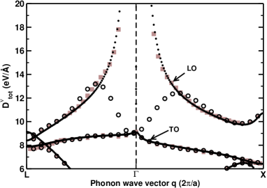
Figure 1: GaAs. Deformation potentials for the total contribution of the three highest valence bands, see Eq. (4). The initial electronic state is at $\mathbf{k}=\Gamma$, and the phonon wave vector $\mathbf{q}$ is varying along high symmetry lines in the BZ. Black line: direct DFPT calculation. Grey squares: Wannier-interpolation extended to polar-optical coupling. Circles: standard Wannier interpolation for metals and non-polar semiconductors.

The Fröhlich interaction is long-range, and thus the electron-phonon matrix elements for long-wavelength longitudinal optical phonons in polar materials are not localized in the real-space Wannier basis. A proof is given in Fig. 1, where the interpolation method of Refs. Giustino et al., 2007; Calandra et al., 2010 is shown to fail for LO phonon as $\mathbf{q}\rightarrow 0$. Indeed, as one can see from Fig. 1, at large $|\mathbf{q}|$ vectors, the character of the electron-phonon matrix elements is completely short-range for all phonon branches including the LO branch and is well reproduced by the standard interpolation method. Calandra et al. (2010). At small $|\mathbf{q}|$ vectors however, instead of the characteristic $1/|\mathbf{q}|$ behaviour, the interpolation method of Ref. Calandra et al., 2010 yields the same values of deformation potentials for the LO and TO branches. This is because, for the highest valence bands, the electron-phonon interaction with long-wavelength LO phonons at $\mathbf{k}=\Gamma$ contains both long-range (Fröhlich) and short-range contributions Yu and Cardona (2001). At vanishing $|\mathbf{q}|$, the short-range contribution is the same for the LO and TO phonons.

The absence of LO/TO splitting within a standard Wannier interpolation procedure is in analogy with the LO/TO splitting of phonon frequencies in polar semiconductors. Indeed, if dynamical matrices are interpolated with a real space cutoff Giannozzi et al. (1991); Baroni et al. (2001), the LO/TO splitting of the phonon modes is absent, and the long-range part of the dynamical matrix needs to be subtracted before Fourier-interpolation into the real space and re-introduced afterwards in order to reproduce the LO/TO splitting Giannozzi et al. (1991); Baroni et al. (2001). We apply similar scheme in the case of electron-phonon matrix elements, with the nonlocal part of the electron-phonon interaction represented by the Vogl model described in the next paragraph.

II.3 The Vogl model

Figure 2: GaAs. LO deformation potentials for the initial electronic state with $\mathbf{k}=X$ and the phonon wave vector changing along the (100) direction: $\mathbf{q}=(q_{x},0,0)2\pi/a$, for $q_{x}\geq$ 0.01. Panel A (top): deformation potentials calculated within DFPT for the lowest conduction band (dashed line) and two lowest valence bands (dot-dashed line, visible in panel B), compared with the deformation potentials calculated from the model of eq. (9) (solid line). Panel B (bottom): The difference between the deformation potentials calculated with DFPT, and the model of eq. (9).

The electron-phonon matrix element of the interaction of electrons with the macroscopic electric field induced by long-wavelength longitudinal optical phonons (the Fröhlich interaction) was derived by Vogl in Ref. Vogl, 1976, for long-wavelength phonons ($\mathbf{q}\rightarrow 0$). The leading contribution, in terms of ascending powers of $q$, to the intraband electron-phonon matrix element, is given by the interaction with a dipole potential ($\propto\frac{1}{|q|}$) screened by the high-frequency dielectric tensor $\mathbf{\epsilon}_{\infty}$ (see Eq. 3.12 of Ref. Vogl, 1976), and reads:

$$g_{diel}^{\nu}(\mathbf{q})=\frac{4\pi ie}{\mathbf{q}\cdot\overleftrightarrow{\mathbf{\epsilon}}_{\infty}\cdot\mathbf{q}}\sum_{s}\sum_{\lambda^{\prime}}q_{\lambda^{{}^{\prime}}}Z_{\lambda^{\prime}\lambda s}\mathbf{e}^{s\nu}_{\lambda}(\mathbf{q})/\sqrt{2M_{s}\omega_{\mathbf{q}\nu}}$$ (9)

The corresponding deformation potential then becomes:

$$D^{\nu}_{diel}(\mathbf{q})=\frac{\sqrt{2\rho\Omega\omega_{\mathbf{q}\nu}}}{\hbar}|g_{diel}^{\nu}(\mathbf{q})|$$ (10)

In eq. (9), $e$ is electronic charge, $Z_{\lambda^{{}^{\prime}}\lambda s}$ is the Born effective charges tensor for atom $s$, and $\lambda,\lambda^{\prime}$ denotes the cartesian components. Among other approximations, it was assumed, in Ref. Vogl, 1976, that:

$$\langle\mathbf{k}+\mathbf{q}m|\mathbf{k}n\rangle=\delta_{mn}+O(q^{2}).$$ (11)

Note that such a relation assumes a smooth and analytic relative phase relation among the $|\mathbf{k},n\rangle$ and $|\mathbf{k+q},m\rangle$ states. Such a requirement is satisfied by the phase choice giving the localised Wannier functions, but not by the arbitrary phase given by the diagonalisation procedure. Furthermore, eq. (11) is the reason why the expression (9) does not depend on the electronic wave vector $\mathbf{k}$ nor on the band indexes of the initial and final electronic states (which are assumed to be the same). Nevertheless, expression (9) describes well the asymptotic behaviour of the electron-phonon matrix elements in polar semiconductors as $\mathbf{q}\rightarrow 0$, as one can see in Fig. 2, where the behaviour of the electron-phonon matrix elements for the lowest conduction band (dashed line) and for the highest valence bands (dot-dashed line) of GaAs calculated within DFPT are compared with the equations (9) and (10) of the model for the Fröhlich interaction along the (100) direction in the Brillouin zone (solid line). At large $q_{x}$, the short-range character of the electron-phonon matrix elements is different for the conduction band and the valence bands, and cannot be described with the model of Eq. (9). At small $q_{x}$, on the contrary, the asymptotic behaviour of the electron-phonon matrix elements for the valence bands and the conduction band becomes similar, and this behaviour is extremely well described by the model of eq. (9).

II.4 Wannier interpolation extended to polar-optical coupling

The method we propose in order to extend the interpolation method of the electron-phonon matrix elements to polar semiconductors is similar to the one described in Ref. Giannozzi et al., 1991 for the interpolation of the force constants in polar materials. The idea is that the long-range contribution to the electron-phonon matrix elements, described with the model of eq. 9, has to be subtracted from the electron-phonon matrix elements before the Fourier transform to real space in eq. (6) and restored after the Fourier transform back to the reciprocal space in eq. (8).

We use the Ewald sum in order to take into account the periodicity properties of the crystal Giannozzi et al. (1991) and define:

$$d^{diel}_{\lambda s}(\mathbf{q})=$$

$$4\pi ie\sum_{\lambda^{{}^{\prime}}}\sum_{\mathbf{G}}\frac{e^{-(\mathbf{q}+\mathbf{G})^{2}/4\alpha}}{(\mathbf{q}+\mathbf{G})\cdot\overleftrightarrow{\mathbf{\epsilon}}_{\infty}\cdot(\mathbf{q}+\mathbf{G})}Z_{\lambda^{\prime}\lambda s}(q_{\lambda^{{}^{\prime}}}+G_{\lambda^{{}^{\prime}}})$$

(12)

Here, $\alpha$ is a convergence parameter (we used $\alpha=$ 5 $(\frac{2\pi}{a})^{2}$ in this work ), and the $\mathbf{G}$ are the reciprocal lattice vectors. The dielectric term, eq. (12), depends only on the phonon wave vector $\mathbf{q}$, and on material characteristics such as the Born effective charges $Z_{\lambda^{{}^{\prime}}\lambda s}$ and the dielectric constant $\mathbf{\epsilon}_{\infty}$, which are calculated within linear response theory Baroni et al. (2001).

Then we subtract $d^{diel}_{\lambda}(\mathbf{q})$ from the intraband Fourier transform of the deformation potential in the optimally smooth subspace, namely we define:

$${\tilde{\cal D}}_{m^{\prime}n^{\prime}}^{\lambda s}(\mathbf{k}+\mathbf{q},\mathbf{k})=\tilde{d}_{m^{\prime}n^{\prime}}^{\lambda s}(\mathbf{k}+\mathbf{q},\mathbf{k})-\delta_{m^{\prime},n^{\prime}}d^{diel}_{\lambda s}(\mathbf{q})$$

We then carry out the transformation in Eq. 8 on the matrix ${\bf{\tilde{\cal D}}}_{m^{\prime}n^{\prime}}^{s}(\mathbf{k}+\mathbf{q},\mathbf{k})$,

$$\mathbf{{\cal D}}_{mn}^{s}(\mathbf{k}+\mathbf{q},\mathbf{k})=\frac{1}{(N_{k})^{2}}\sum_{L}\sum_{\mathbf{R}}\sum_{m^{\prime}n^{\prime}}e^{i\mathbf{k}\mathbf{R}+i\mathbf{q}\mathbf{R}_{L}}$$

$$U_{m^{\prime}m}(\mathbf{k}+\mathbf{q}){\bf{\tilde{\cal D}}}_{m^{\prime}n^{\prime}}^{s}(\mathbf{R},\mathbf{R}_{L})U_{nn^{\prime}}^{*}(\mathbf{k})$$ (14)

where ${\bf{\tilde{\cal D}}}_{m^{\prime}n^{\prime}}^{s}(\mathbf{R},\mathbf{R}_{L})$ is obtained via Eq. 6 with $\tilde{\mathbf{d}}_{m^{\prime}n^{\prime}}^{s}(\mathbf{k}+\mathbf{q},\mathbf{k})$ replaced by ${\tilde{\cal D}}_{m^{\prime}n^{\prime}}^{s}(\mathbf{k}+\mathbf{q},\mathbf{k})$.

Finally we add back $d^{diel}_{\lambda s}(\mathbf{q})$ where now ${\bf q}$ is any phonon wave vector in the Brillouin zone, namely

$$d_{mn}^{\lambda s}(\mathbf{k}+\mathbf{q},\mathbf{k})={\cal D}_{mn}^{\lambda s}(\mathbf{k}+\mathbf{q},\mathbf{k})+d^{diel}_{\lambda s}(\mathbf{q})\delta_{m,n}$$ (15)

In figure 1, the results obtained with the method of Wannier interpolation extended to polar-optical coupling are shown in grey squares. The behaviour of deformation potentials corresponding to LO phonons is well reproduced by the Wannier interpolation extended to polar-optical coupling, in contrast with the standard Wannier interpolation method.

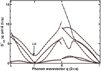
Figure 3: GaAs. Deformation potentials for the total contribution of the three highest valence bands, see eq. (4), multiplied by the modulus of the phonon wave vector $|\mathbf{q}|$. The initial electronic state is at $\mathbf{k}=\Gamma$, and the phonon wave vector $\mathbf{q}$ is varying along high symmetry lines in the BZ. Black line: direct DFPT calculation. Grey squares: our results obtained with the Wannier interpolation extended to the polar-optical coupling.

In figure 3, we show the total deformation potentials for the three highest valence bands of GaAs (${n,m}=2,3,4$), multiplied by the modulus of the phonon wave vector $|\mathbf{q}|$, for all six phonon modes of GaAs. The crystal momentum of the initial electronic state was taken to be $\mathbf{k}=\Gamma$, while the wave vector of the final electronic state $\mathbf{k+q}$ changes as the phonon wavector $\mathbf{q}$ varies along high symmetry lines in the BZ. We chose to multiply deformation potentials by the modulus of $\mathbf{q}$, as, due to the Fröhlich interaction, the deformation potential for the LO phonon tends to infinity as $\frac{1}{|q|}$ and thus the values are very high close to $\Gamma$. In black are represented reference DFPT values, and in grey squares are shown the deformation potentials which were interpolated using our Wannier interpolation method extended to polar-optical coupling. As one can see, the agreement between DFPT calculations and the Wannier-interpolated deformation potentials is excellent. The non-zero value of the deformation potential multiplied by $\mathbf{q}$ at $\mathbf{q}=\Gamma$ is due to the diverging LO-phonon Fröhlich interaction, which is now properly described.

In conclusion, the method of Wannier interpolation extended to polar-optical coupling yields interpolated electron-phonon matrix elements with the same precision as the ”standard” one at large phonon $\mathbf{q}$ vectors, but, in contrast to the standard method, it enables us to correctly describe the diverging LO-phonon Fröhlich interaction at vanishing $\mathbf{q}$.

III Results

III.1 Scattering rates and role of the Fröhlich interaction

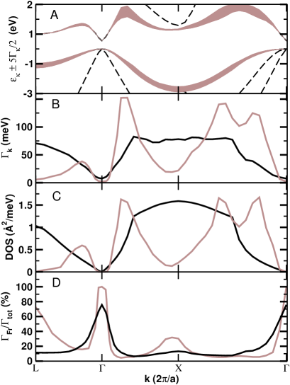
Figure 4: GaAs. Panel A: highest valence and lowest conduction bands broadened by the electron-phonon interaction. The broadening is due to all electron-phonon interaction processes. For the sake of visibility, the calculated broadening $\Gamma_{\mathbf{k}}$ of the electronic bands has been multiplied by 5 in this panel. For panels B-D, the black solid line describes the behaviour of the initial electronic state in the highest valence band and the grey solid line is that of the initial state in the lowest conduction band. Panel B: broadening $\Gamma_{\mathbf{k}}$ due to electron-phonon interaction, as a function of the $\mathbf{k}$ vector of the initial electronic state. Panel C: electronic density of the final states allowed by conservation laws, as a function of the $\mathbf{k}$ vector of the initial electronic state. Panel D: relative contribution of the Fröhlich interaction only to the total broadening. The calculations were done at $T=$300 K.

The method of interpolation of the electron-phonon matrix elements in the Wannier space is necessary when one has to calculate integrals involving many $\mathbf{q}$ points, as it allows to significantly reduce the computational cost, compared to direct DFPT calculation. We have applied the method described in previous section to calculate the total probabilities of the electron-phonon scattering for an electron initially in the lowest conduction band of GaAs, and for a hole initially in the highest valence band of GaAs.

In figure 4, we show the full width at half maximum $\Gamma$ due to the electron-phonon coupling, which was calculated for the lowest conduction band and the highest valence band of GaAs as a function of the $\mathbf{k}$ vector of the initial electronic state, at a temperature of 300 K:

$$\Gamma_{n\mathbf{k}}=\frac{2\pi}{\hbar}\sum_{n^{\prime}}\sum_{\nu}\int_{BZ}d\mathbf{q}|g_{nn^{\prime}}^{\nu}(\mathbf{k},\mathbf{k}\pm\mathbf{q})|^{2}$$

$$\times\delta(\varepsilon_{n^{\prime}\mathbf{k}\pm\mathbf{q}}-\varepsilon_{n\mathbf{k}}\mp\hbar\omega_{\mathbf{q}\nu}){N_{\mathbf{q}}\brace N_{\mathbf{q}}+1}.$$ (16)

Here, $\varepsilon_{n\mathbf{k}}$ are the electronic eigenenergies, and $N_{\mathbf{q}}$ is the phonon occupation number which is described by the Bose-Einstein distribution function. Upper and lower symbols refer to absorbtion and emission, respectively.

In practice, the delta function in eq. (16) was replaced by a Gaussian function in order to calculate numerically the integral in eq. (16). The integration was performed on a $48\times 48\times 48$ $\mathbf{q}$-point grid in the BZ. The calculation was converged with respect to the Gaussian broadening starting from 15 meV broadening. As the pseudopotentials used here reproduce well the respective positions of the minima of the conduction band of GaAs Sjakste et al. (2007b), the Kohn-Sham band structure values at equillibrium were used to calculate the integral (16).

As one can see, the broadening due to electron-phonon coupling varies from a few meV at the bottom of the conduction band or at the top of the valence band (i.e. for $\mathbf{k}$ close to $\Gamma$ point of the BZ), to several tenths of meV at high initial electron energies for the conduction states, or low initial hole energies for the valence band. The behaviour of the total electron-phonon scattering probability is similar to the one of the density of the final electronic states allowed by the energy and momentum conservation laws (panel C), as the probability grows when more final states are available for the electron-phonon scattering. It is, however, not exactly the same, as the electron-phonon matrix elements are not constant over the Brillouin zone.

The contribution due to the Fröhlich interaction is of a few meV and does not change much over the Brillouin zone. It is, however, the dominant scattering process for the electron close to the bottom of the $\Gamma$ or $L$ valleys, and for the hole close to the top of the valence band, as one can see from the Panel D of Fig 4. Away from the band extrema, the intervalley electron-phonon scattering mechanism rapidly becomes the dominant scattering mechanism. This result is in agreement with available literature for low-field transport Stillman et al. (1970). Indeed, at ambient temperatures, the Fröhlich interaction is the dominant scattering mechanism which determines the low-field transport in GaAs Stillman et al. (1970). At high fields, however, the Fröhlich interaction no longer plays the main role, and the intervalley scattering is expected to determine the relaxation dynamics of electrons and/or holes, as can be deduced from Fig. 4. In this respect, GaAs behaviour in similar to that of non-polar semiconductors, i.e. silicon or germanium Jacoboni and Reggiani (1983).

III.2 Relaxation times related to electron-phonon coupling

The widths of the electronic levels due to electron-phonon coupling presented on Fig. 4 can be used to estimate the relaxation times of hot electrons related to electron-phonon scattering. Recently, relaxation time of hot electrons excited in the CB of GaAs close to $\Gamma$ at excess energy $\epsilon_{ex}=0.78$ eV with respect to the CB bottom was found to be 22$\pm$3 fs at 293 K Kanasaki et al. (2014). We find the electron-phonon scattering time $\tau_{\mathbf{k}}=\frac{\hbar}{\Gamma_{\mathbf{k}}}$ to be 30 fs at $\epsilon_{ex}=0.78$ eV, in satisfactory agreement with the experimental result of Ref. Kanasaki et al., 2014.

III.3 Broadenings of some critical points

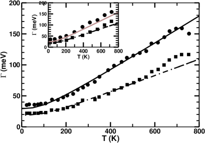
Figure 5: GaAs. Broadening (meV) of the critical point $E_{1}$ as a function of temperature. Points: experimental data of Ref. Gopalan et al., 1987 obtained by fit with the Fano-type excitonic line Lautenschlager et al. (1987). Squares: experimental data of Ref. Gopalan et al., 1987, fit with the two-dimensional critical point modelLautenschlager et al. (1987). Solid black line: this work, Wannier interpolation method extended to polar-optical coupling. Dashed-dotted line: theoretical calculation from Ref. Gopalan et al., 1987 with empirical pseudopotential method. Both theoretical broadenings are due to electron-phonon coupling only and are calculated as the sum of the broadenings of the lowest conduction and highest valence bands, averaged over the four points along the $\Lambda$ direction as explained in the text. The inset represents the same experimental and theoretical results of Ref. Gopalan et al., 1987 as the main figure, with the same notations. Grey solid line on the inset figure: this work, Wannier interpolation method without extension to polar-optical coupling.

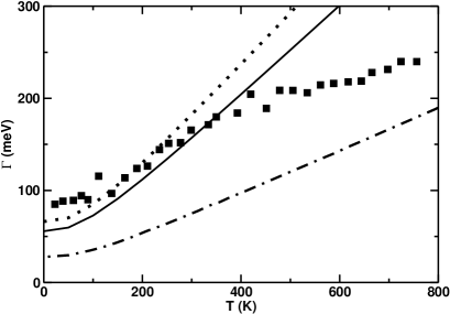
Figure 6: GaAs. Broadening (meV) of the critical point $E_{2}$ as a function of temperature. Squares: experimental data of Ref. Gopalan et al., 1987, fit with two-dimensional critical point modelLautenschlager et al. (1987). Dashed-dotted line: theoretical calculation from Ref. Gopalan et al., 1987 with empirical pseudopotential method. Solid black line: this work, Wannier interpolation method extended to polar-optical coupling, sum of the broadenings of the lowest conduction and highest valence bands, averaged over three points (see text).

The widths of the conduction and valence bands presented in Fig. 4 can be also used to estimate the temperature-dependent broadenings of excitons at critical points in GaAs, attributed mostly to electron-phonon scattering. In principle, one should rely on the many-body excitonic wavefunction to obtain the excitonic lifetime. The latter consists in a combination of products of electron and hole quasiparticle (QP) wavefunctions $\Psi_{e}\Psi_{h}$, linearly mixed through the exchange operator - the electron-hole interaction Onida et al. (2002). Obtaining a precise knowledge of the QP wavefunctions and of the coefficients of the linear combination is out of the scope of this work. Instead, following Ref. Gopalan et al., 1987, we model the excitonic wave function using the DFT wavefunctions of the lowest conduction band for the electron (resp. highest valence band for the hole) and take $\Sigma_{\mathbf{k}=\mathbf{k}_{i}}\psi_{\mathbf{k}c}\psi_{\mathbf{k}v}$ as our excitonic wavefunctions, with the sum limited to a few representative points $\mathbf{k}_{i}$. We then approximate the excitonic lifetime by the sum of the electron and hole lifetime, $\Gamma_{\mathbf{k}c}+\Gamma_{\mathbf{k}v}$. For the critical point $E_{1}$, the width $\Gamma_{\mathbf{k}c}$ (resp. $\Gamma_{\mathbf{k}v}$) of the electronic (resp. hole) level are obtained via eq. (16) with four points $\mathbf{k}_{i}$ equal to $L$,$\frac{3}{4}L$,$\frac{1}{2}L$ and $\frac{1}{4}L$, as done in Ref. Gopalan et al., 1987. In the case of $E_{2}$, only one representative point $\mathbf{k}=2\pi/a(\frac{3}{4},\frac{1}{4},\frac{1}{4})$ was used in Ref. Gopalan et al., 1987. The region in the $\mathbf{k}$ space where valence and conduction bands are parallel and which contributes to the $E_{2}$ point was described in Ref. Alouani et al., 1988. In this work, we decided to take into account three points $\mathbf{k}_{i}$: $(\frac{3}{4},\frac{1}{4},\frac{1}{4})$, $(1,\frac{1}{8},\frac{1}{8})$ and $U$ which belong to the region which contributes to $E_{2}$Alouani et al. (1988).

III.3.1 Broadening of the $E_{1}$ critical point

The resulting broadening $\Gamma_{\mathbf{k}c}+\Gamma_{\mathbf{k}v}$, is reported as a function of temperature for the critical point $E_{1}$ (Fig. 5). As one can see, broadenings of the critical point $E_{1}$ calculated in this work are in satisfactory agreement with the experimental results of Ref. Gopalan et al., 1987. In the case of our calculation, the agreement is best with the experimental data obtained by fit with the Fano-type excitonic shape, whereas the previous theoretical result of Ref. Gopalan et al., 1987 privileged the fit with two-dimensional critical point modelLautenschlager et al. (1987). The question to discriminate between the two methods of fit of the experimental data is, however, out of the scope of present work. Indeed, here we only demonstrate that the calculated widths due to electron-phonon scattering allow to correctly estimate the magnitude of the broadenings of critical points, within the experimental error bar.

In the inset of Fig. 5, we show the result of the calculation of the same broadening of $E_{1}$, but with the standard interpolation method. As one can see, the broadening of $E_{1}$ is slightly lower if the Fröhlich coupling is omitted, however, the overall result is very similar, confirming the statement of the previous section that the scattering of the electrons/holes away from valley minima is dominated not by the Fröhlich, but by the intervalley scattering.

III.3.2 Broadening of the $E_{2}$ critical point

In Fig. 6, we have estimated the broadening of the critical point $E_{2}$ in GaAs. In the case of $E_{2}$, our results (solid line) are very different from the theoretical result obtained with the empirical pseudopotential methodGopalan et al. (1987), and yield a much better agreement with experiment, showing that the experimentally measured broadening of the $E_{2}$ point can be attributed to the electron-phonon scattering. It must be noted down, however, first that only experimental results extracted with the fit with the two-dimensional critical point model are available in this case. Second, the experimental behaviour of the broadening beyond 500 K differs from the one predicted by the calculation.

In dotted line, we show the broadening of the critical point $E_{2}$ estimated in our work with only one point $\mathbf{k}=2\pi/a(\frac{3}{4},\frac{1}{4},\frac{1}{4})$ as was done in Ref. Gopalan et al., 1987. As one can see, the broadening reported with dotted line is similar to the one obtained with three representative points, showing that the result does not depend crucially on the method of averaging and that it remains widely different from the one obtained with empirical pseudopotential.

IV Conclusion

In conclusion, we have presented the description of the extension to polar-optical coupling of the method which allows to interpolate the electron-phonon matrix elements in the space of maximally-localized Wannier functions. The extended method is based on Vogl’s model of the Fröhlich component of the electron-phonon coupling, and allows to interpolate the electron-phonon matrix elements calculated within DFPT in polar semiconductors with excellent precision. We have applied the extended method of interpolation in the case of GaAs, and calculated the widths of the electronic levels due to the electron-phonon coupling for highest conduction and lowest valence band. We have demonstrated that the obtained widths of the electronic levels can be used to estimate the relaxation times of hot electrons and the broadenings of the critical points due to electron-phonon scattering, in good agreement with various experiments. Finally, we have shown that, although the Fröhlich interaction is the dominant scattering process for electrons/holes close to the valley minima, in agreement with low-field transport results, at higher energies, the intervalley scattering is expected to dominate the relaxation dynamics of hot electrons or holes.

V Acknowledgments

This work was supported by the French ANR (project PNANO ACCATTONE) and by the Graphene Flagship. Results have been obtained with Quantum ESPRESSO package Giannozzi et al. (2009); Baroni et al. (2001) and Wannier90 package Marzari et al. (2012). We acknowledge support from the French DGA, and computer time has been granted by GENCI (project 2210) and by Ecole Polytechnique through the LLR-LSI project. J. Sjakste and N. Vast acknowledge with gratitude many discussions with Prof. V. Tyuterev, from Tomsk Pedagogical University, Russia, on the possibility to interpolate electron-phonon matrix elements in polar materials.

References

- Polman and Atwater (2012) A. Polman and H. A. Atwater, Nat. Mater. 11, 174 (2012).
- Delerue and Lannoo (2004) C. Delerue and M. Lannoo, Nanostructures: Theory and Modeling, Nanoscience and Technology (Springer Verlag, Berlin, 2004).
- Zebarjadi et al. (2012) M. Zebarjadi, K. Esfarjani, M. S. Dresselhaus, Z. F. Ren, and G. Chen, Energy and Enviromental Science 5, 5147 (2012).
- Zollner et al. (1989) S. Zollner, J. Kircher, M. Cardona, and S. Gopalan, Solid-State Electronics 32, 1585 (1989).
- Li et al. (1994) G. H. Li, A. R. Goñi, K. Syassen, and M. Cardona, Phys. Rev. B 49, 8017 (1994).
- Steger et al. (2009) M. Steger, A. Yang, D. Karaiskaj, M. Thewalt, E. Haller, J. Ager, M. Cardona, H. Riemann, A. G. N.V. Abrosimov, A. Bulanov, et al., Phys. Rev. B 79, 205210 (2009).
- Gopalan et al. (1987) S. Gopalan, P. Lautenschlager, and M. Cardona, Phys. Rev. B 35, 5577 (1987), URL http://link.aps.org/doi/10.1103/PhysRevB.35.5577.
- Lautenschlager et al. (1987) P. Lautenschlager, M. Garriga, S. Logothetidis, and M. Cardona, Phys. Rev. B 35, 9174 (1987).
- Rossi and Kuhn (2002) F. Rossi and T. Kuhn, Rev. Mod. Phys. 74, 895 (2002).
- Mauri et al. (1996) F. Mauri, O. Zakharov, S. de Gironcoli, S. Louie, and M. Cohen, Phys. Rev. Lett. 77, 1151 (1996).
- Giustino et al. (2007) F. Giustino, J. R. Yates, I. Souza, M. Cohen, and S. G. Louie, Phys. Rev. Lett. 98, 047005 (2007).
- Calandra and Mauri (2011) M. Calandra and F. Mauri, Phys. Rev. Lett. 106, 196406 (2011).
- Piscanec et al. (2004) S. Piscanec, M. Lazzeri, F. Mauri, A. C. Ferrari, and J. Robertson, Phys. Rev. Lett. 93, 185503 (2004).
- Lazzeri and Mauri (2006) M. Lazzeri and F. Mauri, Phys. Rev. Lett. 97, 266407 (2006), URL http://link.aps.org/doi/10.1103/PhysRevLett.97.266407.
- Calandra and Mauri (2007) M. Calandra and F. Mauri, Phys. Rev. B 76, 205411 (2007).
- Bonini et al. (2007) N. Bonini, M. Lazzeri, N. Marzari, and F. Mauri, Phys. Rev. Lett. 99, 176802 (2007), URL http://link.aps.org/doi/10.1103/PhysRevLett.99.176802.
- Papalazarou et al. (2012) E. Papalazarou, J. Faure, J. Mauchain, M. Marsi, A. Taleb-Ibrahimi, I. Reshetnyak, A. van Roekeghem, I. Timrov, N. Vast, B. Arnaud, et al., Phys. Rev. Let. 108, 256808 (2012).
- Faure et al. (2013) J. Faure, J. Mauchain, E. Papalazarou, M. Marsi, D. Boschetto, I. Timrov, N. Vast, Y. Ohtsubo, B. Arnaud, and L. Perfetti, Phys. Rev. B 88, 075120 (2013).
- Baroni et al. (1987) S. Baroni, P. Giannozzi, and A. Testa, Phys. Rev. Lett. 58, 1861 (1987).
- Baroni et al. (2001) S. Baroni, S. de Gironcoli, A. D. Corso, and P. Giannozzi, Rev. Mod. Phys. 73, 515 (2001).
- Sjakste et al. (2007a) J. Sjakste, N. Vast, and V. Tyuterev, Phys. Rev. Lett. 99, 236405 (2007a).
- Tyuterev et al. (2011) V. Tyuterev, S. Obukhov, N. Vast, and J. Sjakste, Phys. Rev. B 84, 035201 (2011).
- Sjakste et al. (2014) J. Sjakste, I. Timrov, P. Gava, N. Mingo, and N. Vast, in Annual Review of Heat Transfer (Begell House Inc., Danbury, CT, USA, 2014), vol. 17, p. 333.
- Murphy-Armando and Fahy (2008) F. Murphy-Armando and S. Fahy, Phys. Rev. B 78, 035202 (2008).
- Vaughan et al. (2012) M. P. Vaughan, F. Murphy-Armando, and S. Fahy, Phys. Rev. B 85, 165209 (2012), URL http://link.aps.org/doi/10.1103/PhysRevB.85.165209.
- Murphy-Armando and Fahy (2011) F. Murphy-Armando and S. Fahy, Journal of Applied Physics 109, 113703 (2011).
- Calandra et al. (2010) M. Calandra, G. Profeta, and F. Mauri, Phys. Rev. B 82, 165111 (2010).
- Marzari et al. (2012) N. Marzari, A. A. Mostofi, J. R. Yates, I. Souza, and D. Vanderbilt, Rev. Mod. Phys. 84, 1419 (2012).
- Casula et al. (2011) M. Casula, M. Calandra, G. Profeta, and F. Mauri, Phys. Rev. Lett. 107, 137006 (2011).
- Margine and Giustino (2013) E. R. Margine and F. Giustino, Phys. Rev. B 87, 024505 (2013).
- Bernardi et al. (2014) M. Bernardi, D. Vigil-Fowler, J. Lischner, J. B. Neaton, and S. G. Louie, Phys. Rev. Lett. 112, 257402 (2014).
- Kanasaki et al. (2014) J. Kanasaki, H. Tanimura, and K. Tanimura, Phys. Rev. Lett. 113, 237401 (2014).
- Sjakste et al. (2013) J. Sjakste, N. Vast, H. Jani, S. Obukhov, and V. Tyuterev, Phys. Status Solidi B 250, 716 (2013).
- Sjakste et al. (2007b) J. Sjakste, V. Tyuterev, and N. Vast, Applied Physics A 86, 301 (2007b), URL http://dx.doi.oorg/10.1007/s00339-006-3786-7.
- Zollner et al. (1990) S. Zollner, S. Gopalan, and M. Cardona, J. Appl. Phys. 68, 1682 (1990).
- Botti et al. (2002) S. Botti, N. Vast, L. Reining, V. Olevano, and L. Andreani, Phys. Rev. Lett. 89, 216803 (2002).
- Yu and Cardona (2001) P. Yu and M. Cardona, Fundamentals of Semiconductors (Springer-Verlag, Berlin New York, 2001).
- Giannozzi et al. (1991) P. Giannozzi, S. de Gironcoli, P. Pavone, and S. Baroni, Phys. Rev. B 43, 7231 (1991).
- Vogl (1976) P. Vogl, Phys. Rev. B 13, 694 (1976).
- Stillman et al. (1970) G. Stillman, C. Wolfe, and J. Dimmock, Journal of Physics and Chemistry of Solids 31, 1199 (1970).
- Jacoboni and Reggiani (1983) C. Jacoboni and L. Reggiani, Rev. Mod. Phys. 55, 645 (1983).
- Onida et al. (2002) G. Onida, L. Reining, and A. Rubio, Rev. Mod. Phys. 74, 601 (2002).
- Alouani et al. (1988) M. Alouani, L. Brey, and N. E. Christensen, Physical Review B 37, 1167 (1988).
- Giannozzi et al. (2009) P. Giannozzi, S. Baroni, N. Bonini, M. Calandra, R. Car, C. Cavazzoni, D. Ceresoli, G. Chiarotti, M. Cococcioni, I. Dabo, A. Dal Corso, S. de Gironcoli, S. Fabris, G. Fratesi, R. Gebauer, U. Gerstmann, C. Gougoussis, A. Kokalj, M. Lazzeri, L. Martin-Samos, N. Marzari, F. Mauri, R. Mazzarello, S. Paolini, A. Pasquarello, L. Paulatto, C. Sbraccia, S. Scandolo, G. Sclauzero, A. Seitsonen, A. Smogunov, P. Umari, R. Wentzcovitch, Journal of Physics: Condensed Matter 21, 395502 (2009).