Adaptive vertex-centered finite volume methods
with convergence rates

Abstract.

We consider the vertex-centered finite volume method with first-order conforming ansatz functions. The adaptive mesh-refinement is driven by the local contributions of the weighted-residual error estimator. We prove that the adaptive algorithm leads to linear convergence with generically optimal algebraic rates for the error estimator and the sum of energy error plus data oscillations. While similar results have been derived for finite element methods and boundary element methods, the present work appears to be the first for adaptive finite volume methods, where the lack of the classical Galerkin orthogonality leads to new challenges.

1. Introduction

1.1. Finite volume method

A classical finite volume method (FVM) describes numerically a conservation law of an underlying model problem, which might be described by a partial differential equation (PDE). In particular, it naturally preserves local conservation of the numerical fluxes. Therefore, FVMs are well-established in the engineering community (fluid mechanics). Even though the FVM has a wide range of applications the numerical analysis is less developed than for the more prominent finite element method (FEM). There exist different versions of the FVM like the cell-centered FVM, which basically yields to a piecewise constant approximation of the unknown solution on a primal mesh. For more details we refer to [EGH00]. The so-called vertex-centered FVM (finite volume element method, box method) belongs to the other big family of FVMs, where one usually introduces an additional dual mesh around the nodes for the approximation. In this work, we focus on the lowest-order vertex-centered finite volume method (from now on only FVM) for some elliptic model problem in ${\mathbb{R}}^{d}$, $d=2,3$. The first relevant mathematical analysis of this method started with the works [BR87, Hac89, Cai91].

1.2. A posteriori error estimation and adaptive mesh-refinement

Accurate a posteriori error estimation and related adaptive mesh-refinement is one fundamental column of modern scientific computing. On the one hand, the a posteriori error estimator allows to monitor whether a numerical approximation is sufficiently accurate, even though the exact solution is unknown. On the other hand, it allows to adapt the discretization to resolve possible singularities most effectively. Over the last few years, the mathematical understanding of adaptive mesh-refinement has matured. It has been proved that adaptive procedures for the finite element method (FEM) as well as for the boundary element method (BEM) lead to optimal convergence behavior of the numerical scheme; see, e.g., [Dör96, MNS00, BDD04, Ste07, CKNS08, FFP14] for FEM, [FKMP13, FFK⁺14, FFK⁺15, Gan13] for BEM, and [CFPP14] for some general framework.

In this work, we analyze an adaptive mesh-refining algorithm of the type

$$\boxed{\tt SOLVE}\quad\Longrightarrow\quad\boxed{\tt ESTIMATE}\quad\Longrightarrow\quad\boxed{\tt MARK}\quad\Longrightarrow\quad\boxed{\tt REFINE}$$ (1)

in the frame of the FVM (Algorithm 4). Given a conforming triangulation ${\mathcal{T}}_{\ell}$, the module SOLVE uses FVM to compute a discrete approximation $u_{\ell}$ to the solution $u$ of the PDE. For the ease of presentation, we assume that the linear system is solved exactly, although, in the spirit of [CFPP14, Section 7], stopping criteria for iterative solvers can be included into our analysis. The module ESTIMATE employs a weighted-residual error estimator $\eta_{\ell}$ from [CLT05, XZ06] which is also well-studied in the context of adaptive finite element methods [Ste07, CKNS08, FFP14]. The module MARK uses the Dörfler marking criterion introduced in [Dör96], to mark elements for refinement, where the local error appears to be large. Unlike common algorithms for FEM and BEM, we follow [MNS00] and also mark elements with respect to the data oscillations to overcome the lack of the Galerkin orthogonality. Finally, the module REFINE employs newest vertex bisection (NVB) to refine the marked elements and to generate a new conforming triangulation ${\mathcal{T}}_{\ell+1}$ which better resolves the present singularities.

1.3. Contributions of the present work

Iteration of the adaptive loop (1) provides a sequence of successively refined triangulations ${\mathcal{T}}_{\ell}$ together with the corresponding FVM solutions $u_{\ell}$ and the a posteriori error estimators $\eta_{\ell}$. Theorem 7 below proves that this adaptive iteration leads to linear convergence in the sense of

$$\eta_{\ell+n}\leq Cq^{n}\,\eta_{\ell}\quad\text{for all }\ell,n\in{\mathbb{N}}_{0}$$ (2)

with some independent constants $C>0$ and $0<q<1$. Under an additional assumption on the marking which can be monitored a posteriori, we prove optimal convergence behavior

$$\eta_{\ell}\leq C\,(\#{\mathcal{T}}_{\ell}-\#{\mathcal{T}}_{0})^{-s}$$ (3)

for each “possible” algebraic rate $s>0$ (in the sense of certain nonlinear approximation classes which are defined in Section 2.6 below), where $\#{\mathcal{T}}_{\ell}$ denotes the number of elements in ${\mathcal{T}}_{\ell}$. These results can be equivalently stated with respect to the sum of energy error plus data oscillations, which is usually done in the FEM literature [Ste07, CKNS08, FFP14], since

$$C^{-1}\,\eta_{\ell}\leq\min_{v_{\ell}}\big{(}|||u-v_{\ell}|||+{\rm osc}_{\ell}(v_{\ell})\big{)}\leq|||u-u_{\ell}|||+{\rm osc}_{\ell}(u_{\ell})\leq C\,\eta_{\ell};$$ (4)

see Theorem 2 below. We note that (4) in particular provides a generalized Céa lemma which states that the FVM solution $u_{\ell}$ is quasi-optimal with respect to the so-called total error, i.e., the sum of energy error plus data oscillations. Since (4) is also known for the FEM (see, e.g., [FFP14, Lemma 5.1]), this reveals that FEM and FVM lead to equivalent errors in the sense of

$$C^{-1}\,\big{(}|||u-u_{\ell}|||+{\rm osc}_{\ell}(u_{\ell})\big{)}\leq|||u-u_{\ell}^{\rm FEM}|||+{\rm osc}_{\ell}(u_{\ell}^{\rm FEM})\leq C\,\big{(}|||u-u_{\ell}|||+{\rm osc}_{\ell}(u_{\ell})\big{)},$$ (5)

where $u_{\ell}^{\rm FEM}$ is the FEM solution with respect to the FVM space. This complements recent results which compare the total errors of different FEM discretizations [CPS12, CKPS15].

Unlike the results for FEM and BEM, the novel Céa-type estimate (4) as well as our result (2)–(3) on adaptive FVM requires the additional assumption that the initial triangulation ${\mathcal{T}}_{0}$ is sufficiently fine. We note, however, that such an assumption is also required to prove well-posedness of the FVM in general and thus appears naturally.

Prior to this work, a posteriori error estimates for the FVM for elliptic model problems are derived in [CLT05, XZ06, Zou10]; see also [Era13, Remark 6.1] and [Era13, Conclusions] for estimates which are robust with respect to the lower-order convection and reaction terms. To the best of the authors’ knowledge, convergence of an adaptive 2D FVM has only been analyzed in the yet unpublished preprint [XZ06]. The latter is concerned with convergence only and the analysis follows [MNS00] and relies on a discrete efficiency estimate and hence on the so-called interior node property of the mesh-refinement. Contrary to [XZ06], our analysis extends the ideas of [CKNS08] and provides a contraction property for the weighted sum of energy error, weighted-residual error estimator, and data oscillations. Therefore, our analysis covers in particular standard NVB, where marked elements are refined by one bisection.

We finally note that residual error estimators have also been developed for the cell-centered finite volume method [Nic05, EP08, Voh08]. These a posteriori estimators rely on an interpolatory post-processing of the original piecewise constant cell-centered finite volume approximation. Thus, a thorough adaptive convergence analysis requires additional ideas to extend and adapt the analysis presented below.

1.4. General notation

We use $\lesssim$ to abbreviate $\leq$ up to some (generic) multiplicative constant which is clear from the context. Moreover, $\simeq$ abbreviates that both estimates $\lesssim$ and $\gtrsim$ hold. Throughout, the mesh-dependence of (discrete) quantities is explicitly stated by use of appropriate indices, e.g., $u_{\times}$ is the FVM solution for the triangulation ${\mathcal{T}}_{\times}$ and $\eta_{\ell}$ is the error estimator with respect to the triangulation ${\mathcal{T}}_{\ell}$.

2. Model problem & main results

2.1. Model problem

Let $\Omega\subset{\mathbb{R}}^{d}$, $d=2,3$, be a bounded and connected Lipschitz domain with boundary $\Gamma:=\partial\Omega$. As model problem, we consider the following stationary diffusion problem: Given $f\in L^{2}(\Omega)$, find $u\in H^{1}(\Omega)$ such that

$$-{\rm div}\mathbf{A}\nabla u =f\quad\text{in }\Omega,$$ (6a)

$$u =0\quad\text{on }\Gamma.$$ (6b)

We suppose that the diffusion matrix $\mathbf{A}=\mathbf{A}(x)\in{\mathbb{R}}^{d\times d}$ is bounded, symmetric, and uniformly positive definite, i.e., there exist constants $\lambda_{\rm min},\lambda_{\rm max}>0$ such that

$$\lambda_{\rm min}\,|\mathbf{v}|^{2}\leq\mathbf{v}^{T}\mathbf{A}(x)\mathbf{v}\leq\lambda_{\rm max}\,|\mathbf{v}|^{2}\quad\text{for all }\mathbf{v}\in{\mathbb{R}}^{d}\text{ and almost all }x\in\Omega.$$ (7)

For convergence of our FVM and well-posedness of the residual error estimator, we additionally require that $\mathbf{A}(x)$ is piecewise Lipschitz continuous, i.e.,

$$\mathbf{A}\in W^{1,\infty}(T)^{d\times d}\quad\text{for all}\quad T\in{\mathcal{T}}_{0},$$ (8)

where ${\mathcal{T}}_{0}$ is some given initial triangulation of $\Omega$; see Section 2.5 below.

The weak formulation of the model problem (6) reads: Find $u\in H^{1}_{0}(\Omega)$ such that

$${\mathcal{A}}(u,v):=(\mathbf{A}\nabla u\hskip 1.42262pt,\nabla v)_{\Omega}=(f\hskip 1.42262pt,v)_{\Omega}\quad\text{for all }v\in H^{1}_{0}(\Omega),$$ (9)

where $(\phi\hskip 1.42262pt,\psi)_{\Omega}=\int_{\Omega}\phi(x)\psi(x)\,dx$ denotes the $L^{2}$-scalar product. According to our assumptions (7) on $\mathbf{A}$, the bilinear form ${\mathcal{A}}(\cdot,\cdot)$ is continuous and elliptic on $H^{1}_{0}(\Omega)$. Therefore, existence and uniqueness of the solution $u\in H^{1}_{0}(\Omega)$ of (9) follow from the Lax-Milgram theorem. Moreover, $|||v|||^{2}:={\mathcal{A}}(v,v)$ defines the so-called energy norm which is an equivalent norm on $H^{1}_{0}(\Omega)$. We shall use the notation $|||v|||_{\omega}^{2}:=\int_{\omega}\mathbf{A}\nabla v\cdot\nabla v$ for the energy norm on subdomains $\omega\subseteq\Omega$, i.e., $|||v|||=|||v|||_{\Omega}$. According to (7), it holds $|||v|||_{\omega}\simeq\|\nabla v\|_{L^{2}(\omega)}$.

2.2. Triangulation

Throughout, ${\mathcal{T}}_{\times}$ denotes a conforming triangulation of $\Omega$ into non-degenerated closed simplices $T\in{\mathcal{T}}_{\times}$ (i.e., triangles for $d=2$, tetrahedra for $d=3$), ${\mathcal{N}}_{\times}$ is the corresponding set of nodes, and ${\mathcal{F}}_{\times}$ is the corresponding set of facets (i.e., edges for $d=2$ and triangular faces for $d=3$). We suppose that ${\mathcal{T}}_{\times}$ is $\sigma$-shape regular, i.e.,

$$\max_{T\in{\mathcal{T}}_{\times}}\frac{{\rm diam}(T)^{d}}{|T|}\leq\sigma<\infty.$$ (10)

Here, ${\rm diam}(T):=\max\big{\{}|x-y|\,:\,x,y\in T\big{\}}$ denotes the Euclidean diameter and $|T|$ is the area of $T$. Additionally, we assume that the triangulation ${\mathcal{T}}_{\times}$ is aligned with the discontinuities of the coefficient matrix $\mathbf{A}$, i.e., (8) holds with ${\mathcal{T}}_{0}$ replaced by ${\mathcal{T}}_{\times}$. We note that this follows from (8) and the mesh-refinement used; see Section 2.6. Associated with ${\mathcal{T}}_{\times}$ is the local mesh-size function $h_{\times}\in L^{\infty}(\Omega)$ which is defined by $h_{\times}|_{T}:=h_{T}:=|T|^{1/d}$. Note that $\sigma$-shape regularity (10) yields $h_{T}\simeq{\rm diam}(T)$.

For the nodes ${\mathcal{N}}_{\times}$, we introduce the partition ${\mathcal{N}}_{\times}={\mathcal{N}}_{\times}^{\Gamma}\cup{\mathcal{N}}_{\times}^{\Omega}$ into all boundary nodes ${\mathcal{N}}_{\times}^{\Gamma}:={\mathcal{N}}_{\times}\cap\Gamma$ and all interior nodes ${\mathcal{N}}_{\times}^{\Omega}:={\mathcal{N}}_{\times}\backslash{\mathcal{N}}_{\times}^{\Gamma}$.

For the facets ${\mathcal{F}}_{\times}$, we introduce the partition ${\mathcal{F}}_{\times}={\mathcal{F}}_{\times}^{\Gamma}\cup{\mathcal{F}}_{\times}^{\Omega}$ into all boundary facets ${\mathcal{F}}_{\times}^{\Gamma}:=\big{\{}F\in{\mathcal{F}}_{\times}\,:\,F\subset\Gamma\big{\}}$ and all interior facets ${\mathcal{F}}_{\times}^{\Omega}:={\mathcal{F}}_{\times}\backslash{\mathcal{F}}_{\times}^{\Gamma}$. Finally, for an element $T\in{\mathcal{T}}_{\times}$, we denote by ${\mathcal{F}}_{T}:=\big{\{}F\in{\mathcal{F}}_{\times}\,:\,F\subset\partial T\big{\}}\subseteq{\mathcal{F}}_{\times}$ the set of all facets of $T$.

\psfrag{v1}[c][c]{\small$V_{1}$}\psfrag{v2}[c][c]{\small$V_{2}$}\psfrag{v3}[c][c]{\small$V_{3}$}\psfrag{v4}[c][c]{\small$V_{4}$}\psfrag{v5}[c][c]{\small$V_{5}$}\psfrag{v6}[c][c]{\small$V_{6}$}\psfrag{v7}[c][c]{\small$V_{7}$}\psfrag{v}[c][c]{\small$V$}\includegraphics[width=173.44534pt]{figures/primaldual.eps}

(a) Dual mesh ${\mathcal{T}}_{\times}^{*}$.

\psfrag{v1}[c][c]{\small$V_{1}$}\psfrag{v2}[c][c]{\small$V_{2}$}\psfrag{v3}[c][c]{\small$V_{3}$}\psfrag{v4}[c][c]{\small$V_{4}$}\psfrag{v5}[c][c]{\small$V_{5}$}\psfrag{v6}[c][c]{\small$V_{6}$}\psfrag{v7}[c][c]{\small$V_{7}$}\psfrag{v}[c][c]{\small$V$}\psfrag{V}[c][c]{\small$V$}\includegraphics[width=173.44534pt]{figures/star.eps}

(b) Edges of ${\mathcal{F}}_{V,\times}$.

Figure 1. Local construction of the dual mesh ${\mathcal{T}}^{*}_{\times}$ from the primal mesh ${\mathcal{T}}_{\times}$ in 2D: The dashed lines are the boundaries of the induced control volumes $V_{i}\in{\mathcal{T}}^{*}_{\times}$, which are associated with the nodes $a_{i}\in{\mathcal{N}}_{\times}$ of ${\mathcal{T}}_{\times}$ (left). For $V\in{\mathcal{T}}_{\times}^{*}$, the set ${\mathcal{F}}_{V,\times}$ consists of the bold lines which are parts of edges in ${\mathcal{F}}_{\times}$ (right).

\psfrag{T}[c][c]{\small$T$}\psfrag{cT}[c][c]{\small$c_{T}$}\psfrag{ai}[c][c]{\small$a_{i}$}\psfrag{Q1}[c][c]{\small$Q_{1}$}\psfrag{Q2}[c][c]{\small$Q_{2}$}\psfrag{Q3}[c][c]{\small$Q_{3}$}\psfrag{cE1}[c][c]{\small$c_{F_{1}}$}\psfrag{cE2}[c][c]{\small$c_{F_{2}}$}\psfrag{cE3}[c][c]{\small$c_{F_{3}}$}\psfrag{m1}[c][c]{\small$m_{1}$}\psfrag{m2}[c][c]{\small$m_{2}$}\psfrag{m3}[c][c]{\small$m_{3}$}\includegraphics[width=173.44534pt]{figures/dualmesh3d.eps}

(a) Dual mesh ${\mathcal{T}}^{*}_{\times}$.

\psfrag{T}[c][c]{\small$T$}\psfrag{cT}[c][c]{\small$c_{T}$}\psfrag{ai}[c][c]{\small$a_{i}$}\psfrag{Q1}[c][c]{\small$Q_{1}$}\psfrag{Q2}[c][c]{\small$Q_{2}$}\psfrag{Q3}[c][c]{\small$Q_{3}$}\psfrag{cE1}[c][c]{\small$c_{F_{1}}$}\psfrag{cE2}[c][c]{\small$c_{F_{2}}$}\psfrag{cE3}[c][c]{\small$c_{F_{3}}$}\psfrag{m1}[c][c]{\small$m_{1}$}\psfrag{m2}[c][c]{\small$m_{2}$}\psfrag{m3}[c][c]{\small$m_{3}$}\psfrag{z1}[c][c]{\small$\zeta_{1}$}\psfrag{z2}[c][c]{\small$\zeta_{2}$}\psfrag{z3}[c][c]{\small$\zeta_{3}$}\includegraphics[width=173.44534pt]{figures/dualmesh3dEEV.eps}

(b) Some faces $\zeta_{j}$ of ${\mathcal{F}}_{V_{i},\times}$

Figure 2. Local construction of the dual mesh ${\mathcal{T}}^{*}_{\times}$ from the primal mesh ${\mathcal{T}}_{\times}$ in 3D: For a node $a_{i}\in{\mathcal{N}}_{\times}$ of $T$, the center of gravity $c_{T}$ of $T$ is connected with the centers of gravity $c_{F_{j}}$ of the three adjacent faces $F\in{\mathcal{F}}_{T}$. Moreover, these centers are connected to the midpoints $m_{k}$ of the three edges which meet in $a_{i}$. Together with the edges from these midpoints to $a_{i}$, we get the cuboid $V_{i}\cap T\not=\emptyset$ (left). The three dark-gray faces $Q_{1}$, $Q_{2}$, and $Q_{3}$ are part of the boundary $\partial V_{i}$ of the box $V_{i}$ (left). The light-gray faces $\zeta_{1}$, $\zeta_{2}$, and $\zeta_{3}$ belong to the set ${\mathcal{F}}_{V_{i},\times}$ and are part of faces in ${\mathcal{F}}_{\times}$ (right).

2.3. Dual mesh

In contrast to standard FEM, our FVM discretization additionally needs the so-called dual mesh ${\mathcal{T}}^{*}_{\times}$ which is built from the conforming triangulation ${\mathcal{T}}_{\times}$. In 2D, connecting the center of gravity of an element $T\in{\mathcal{T}}_{\times}$ with the (edge) midpoint of $F\in{\mathcal{F}}_{T}$, we obtain ${\mathcal{T}}^{*}_{\times}$ whose boxes (elements) $V\in{\mathcal{T}}^{*}_{\times}$ are non-degenerate closed polygons; see Figure 11(a). In 3D, we connect the center of gravity of an element $T\in{\mathcal{T}}_{\times}$ with the centers of gravity of the four faces $F\in{\mathcal{F}}_{T}$. Furthermore, each center of gravity of a face $F\in{\mathcal{F}}_{T}$ is connected by straight lines to the midpoints of the edges of the face $F$. Figure 22(a) shows the contribution of some element $T\in{\mathcal{T}}_{\times}$ with node $a_{i}$ to the box $V_{i}\in{\mathcal{T}}^{*}_{\times}$.

Note that there is a unique correspondence between the nodes $a_{i}\in{\mathcal{N}}_{\times}$ of the primal mesh ${\mathcal{T}}_{\times}$ and the boxes $V_{i}\in{\mathcal{T}}^{*}_{\times}$ of the dual mesh, namely $V_{i}\cap{\mathcal{N}}_{\times}=\{a_{i}\}$. Furthermore, we define ${\mathcal{F}}_{V,\times}:=\big{\{}F\cap V\,:\,F\in{\mathcal{F}}_{\times}\big{\}}$ for all $V\in{\mathcal{T}}^{*}_{\times}$; see Figure 11(b) for 2D.

For 3D, Figure 22(b) shows three faces $\zeta_{1}$, $\zeta_{2}$, and $\zeta_{3}$ of ${\mathcal{F}}_{V_{i},\times}$, $V_{i}\in{\mathcal{T}}^{*}_{\times}$. Note that

$$\bigcup_{T\in{\mathcal{T}}_{\times}}T=\overline{\Omega}=\bigcup_{V\in{\mathcal{T}}_{\times}^{*}}V\quad\text{and}\quad\bigcup_{F\in{\mathcal{F}}_{\times}}F=\bigcup_{V\in{\mathcal{T}}^{*}_{\times}}\bigcup_{F\in{\mathcal{F}}_{V,\times}}F.$$ (11)

2.4. Vertex-centered finite volume method (FVM)

Given the conforming triangulation ${\mathcal{T}}_{\times}$ and the corresponding dual mesh ${\mathcal{T}}^{*}_{\times}$, we define the space of all ${\mathcal{T}}_{\times}$-piecewise affine and globally continuous functions

$$\SS^{1}({\mathcal{T}}_{\times}):=\big{\{}v\in{\mathcal{C}}(\Omega)\,:\,v|_{T}\text{ affine for all }T\in{\mathcal{T}}_{\times}\big{\}}\subset H^{1}(\Omega)$$

as well as the space of all ${\mathcal{T}}_{\times}^{*}$-piecewise constant functions

$${\mathcal{P}}^{0}({\mathcal{T}}^{*}_{\times}):=\big{\{}v\in L^{2}(\Omega)\,:\,v|_{V}\text{ constant for all }V\in{\mathcal{T}}^{*}_{\times}\big{\}}.$$

For the FVM discretization, we consider the subspaces which respect the homogeneous Dirichlet conditions of (6), i.e.,

$$\SS^{1}_{0}({\mathcal{T}}_{\times}):=\big{\{}v\in\SS^{1}({\mathcal{T}}_{\times})\,:\,v|_{\Gamma}=0\big{\}}\subset H^{1}_{0}(\Omega)\text{ and }{\mathcal{P}}^{0}_{0}({\mathcal{T}}_{\times}^{*}):=\big{\{}v\in{\mathcal{P}}^{0}({\mathcal{T}}_{\times}^{*})\,:\,v|_{\Gamma}=0\big{\}}.$$

The formal idea of the FVM reads as follows: If we integrate the strong form (6) over each dual element $V\in{\mathcal{T}}^{*}_{\times}$ and apply the divergence theorem, we get a balance equation for the model problem. The FVM approximates $u\in H^{1}_{0}(\Omega)$ by some conforming approximation $u_{\times}\in\SS^{1}_{0}({\mathcal{T}}_{\times})$ of the balance equation. With the aid of test functions in ${\mathcal{P}}^{0}_{0}({\mathcal{T}}_{\times}^{*})$, we formalize this with the bilinear form

$$\begin{split}{\mathcal{A}}_{\times}(v_{\times},v_{\times}^{*}):=-\sum_{a_{i}\in{\mathcal{N}}_{\times}^{\Omega}}v_{\times}^{*}|_{V_{i}}\int_{\partial V_{i}}\mathbf{A}\nabla v_{\times}\cdot{\mathbf{n}}\,ds\quad\text{for all }v_{\times}\in\SS^{1}_{0}({\mathcal{T}}_{\times})\text{ and }v_{\times}^{*}\in{\mathcal{P}}^{0}_{0}({\mathcal{T}}_{\times}^{*}).\end{split}$$ (12)

The right-hand side reads

$$\sum_{a_{i}\in{\mathcal{N}}_{\times}^{\Omega}}v_{\times}^{*}|_{V_{i}}\int_{V_{i}}f\,dx=(f\hskip 1.42262pt,v_{\times}^{*})_{\Omega}\quad\text{for all }v_{\times}^{*}\in{\mathcal{P}}^{0}_{0}({\mathcal{T}}_{\times}^{*}).$$

Throughout, if ${\mathbf{n}}$ appears in a boundary integral, it denotes the unit normal vector to the boundary pointing outward the respective domain. Now, the FVM discretization reads: Find $u_{\times}\in\SS^{1}_{0}({\mathcal{T}}_{\times})$ such that

$${\mathcal{A}}_{\times}(u_{\times},v_{\times}^{*}) =(f\hskip 1.42262pt,v_{\times}^{*})_{\Omega}\quad\text{for all }v_{\times}^{*}\in{\mathcal{P}}^{0}_{0}({\mathcal{T}}_{\times}^{*}).$$ (13)

It is well-known that there exists a constant $H>0$ such that (13) admits a unique solution $u_{\times}\in\SS^{1}_{0}({\mathcal{T}}_{\times})$ provided that ${\mathcal{T}}_{\times}$ is sufficiently fine, i.e., $\|h_{\times}\|_{L^{\infty}(\Omega)}\leq H$; see Lemma 14 below. The convergence of the FVM is usually proved under certain regularity assumptions, e.g., $u\in H^{1}_{0}(\Omega)\cap H^{1+\varepsilon}(\Omega)$ for some $\varepsilon>0$; see, e.g., [ELL02, Theorem 3.3.]. As a side result of our analysis, Theorem 3 below proves convergence of the total error (i.e., energy error plus data oscillations) without any regularity assumptions.

2.5. Weighted-residual error estimator

With ${\rm div}_{\times}$ denoting the ${\mathcal{T}}_{\times}$-piecewise divergence operator, we define the volume residual by

$$R_{\times}(v_{\times})|_{T}=(f+{\rm div}_{\times}\mathbf{A}\nabla v_{\times})|_{T}\quad\text{for all }T\in{\mathcal{T}}_{\times}\text{ and all }v_{\times}\in\SS^{1}_{0}({\mathcal{T}}_{\times}).$$ (14)

Throughout, we abbreviate ${\rm div}_{\times}\mathbf{A}\nabla v_{\times}:={\rm div}_{\times}(\mathbf{A}\nabla v_{\times})$ to ease the readability. Let $[[\cdot]]$ denote the normal jump across an interior facet $F=T\cap T^{\prime}\in{\mathcal{F}}_{\times}^{\Omega}$, i.e., $[[\boldsymbol{g}]]|_{F}=\boldsymbol{g}|_{T}\cdot{\mathbf{n}}_{T}+\boldsymbol{g}|_{T^{\prime}}\cdot{\mathbf{n}}_{T^{\prime}}$, where, e.g., $\boldsymbol{g}|_{T}$ denotes the trace of $\boldsymbol{g}$ from $T$ onto $F$ and ${\mathbf{n}}_{T}$ is the outer normal of $T$ on $F$. Then, we define the facet residual or normal jump by

$$J_{\times}(v_{\times})|_{F}=[[\mathbf{A}\nabla v_{\times}]]|_{F}\quad\text{ for all }F\in{\mathcal{F}}_{\times}^{\Omega}\text{ and all }v_{\times}\in\SS^{1}_{0}({\mathcal{T}}_{\times}).$$ (15)

For all $v_{\times}\in\SS^{1}_{0}({\mathcal{T}}_{\times})$, we define the weighted-residual error estimator as for the FEM

$$\eta_{\times}(v_{\times})^{2}=\eta_{\times}({\mathcal{T}}_{\times},v_{\times})^{2}\quad\text{with}\quad\eta_{\times}(\mathcal{U}_{\times},v_{\times})^{2}=\sum_{T\in\mathcal{U}_{\times}}\eta_{\times}(T,v_{\times})^{2}\quad\text{for all }\mathcal{U}_{\times}\subseteq{\mathcal{T}}_{\times},$$ (16)

where

$$\eta_{\times}(T,v_{\times})^{2}=h_{T}^{2}\,\|f+{\rm div}_{\times}\mathbf{A}\nabla v_{\times}\|_{L^{2}(T)}^{2}+h_{T}\,\|[[\mathbf{A}\nabla v_{\times}]]\|_{L^{2}(\partial T\backslash\Gamma)}^{2};$$ (17)

cf., e.g., [AO00, Ver13]. For $v_{\times}=u_{\times}$ being the discrete FVM solution, we abbreviate the notation and omit this argument, e.g., $\eta_{\times}:=\eta_{\times}(u_{\times})$ and $\eta_{\times}(T):=\eta(T,u_{\times})$.

Let $\Pi_{\times}$ denote the elementwise or facetwise integral mean operator, i.e.,

$$(\Pi_{\times}v)|_{\tau}=\frac{1}{|\tau|}\int_{\tau}v\,dx\quad\text{for all }\tau\in{\mathcal{T}}_{\times}\cup{\mathcal{F}}_{\times}\text{ and all }v\in L^{2}(\tau).$$ (18)

Recall that $\Pi_{\times}$ is the elementwise $L^{2}$-orthogonal projection onto the constants, i.e.,

$$\|v-\Pi_{\times}v\|_{L^{2}(\tau)}=\min_{c\in{\mathbb{R}}}\|v-c\|_{L^{2}(\tau)}\leq\|v\|_{L^{2}(\tau)}\quad\text{for all }\tau\in{\mathcal{T}}_{\times}\cup{\mathcal{F}}_{\times}\text{ and all }v\in L^{2}(\tau).$$ (19)

With $\Pi_{\times}$, we define the data oscillations

$${\rm osc}_{\times}(v_{\times})^{2}={\rm osc}_{\times}({\mathcal{T}}_{\times},v_{\times})^{2}\text{ with }{\rm osc}_{\times}(\mathcal{U}_{\times},v_{\times})^{2}=\sum_{T\in\mathcal{U}_{\times}}{\rm osc}_{\times}(T,v_{\times})^{2}\text{ for all }\mathcal{U}_{\times}\subseteq{\mathcal{T}}_{\times},$$

where

$${\rm osc}_{\times}(T,v_{\times})^{2}=h_{T}^{2}\,\|(1-\Pi_{\times})(f+{\rm div}_{\times}\mathbf{A}\nabla v_{\times})\|_{L^{2}(T)}^{2}+h_{T}\,\|(1-\Pi_{\times})[[\mathbf{A}\nabla v_{\times}]]\|_{L^{2}(\partial T\backslash\Gamma)}^{2}.$$ (20)

Again, we abbreviate the notation for $v_{\times}=u_{\times}$ being the FVM solution, e.g., ${\rm osc}_{\times}:={\rm osc}_{\times}(u_{\times})$ and ${\rm osc}_{\times}(T):={\rm osc}_{\times}(T,u_{\times})$. Moreover, we stress the elementwise estimate

$${\rm osc}_{\times}(T,v_{\times})\leq\eta_{\times}(T,v_{\times})\quad\text{for all }T\in{\mathcal{T}}_{\times}\text{ and all }v_{\times}\in\SS^{1}_{0}({\mathcal{T}}_{\times})$$ (21)

which immediately follows from (19). The following result is proved in [XZ06, Theorem 2.4] and [XZ06, Theorem 2.6]; see also [CLT05, Theorem 3.1] and [CLT05, Theorem 3.3].

Proposition 1 (reliability and efficiency).

The estimator $\eta_{\times}$ satisfies reliability

$$|||u-u_{\times}|||^{2}\leq C_{\rm rel}\,\eta_{\times}^{2}$$ (22)

as well as efficiency

$$C_{\rm eff}^{-1}\,\eta_{\times}^{2}\leq|||u-u_{\times}|||^{2}+{\rm osc}_{\times}^{2}.$$ (23)

The constants $C_{\rm rel},C_{\rm eff}>0$ depend only on $\sigma$-shape regularity of ${\mathcal{T}}_{\times}$ and on the assumptions (7)–(8) on $\mathbf{A}$. ∎

The first contribution of the present work is the following Céa-type quasi-optimality of FVM with respect to the total error (i.e., sum of energy error plus data oscillations). In particular, this implies that the total errors of FVM and FEM are equivalent, see (5). The proof of the theorem is given in Section 3.6.

Theorem 2.

There exists $H>0$ such that the following statement is valid provided that ${\mathcal{T}}_{\times}$ is sufficiently fine, i.e., $\|h_{\times}\|_{L^{\infty}(\Omega)}\leq H$: There is a constant $C_{\rm tot}>0$ such that

$$C_{\rm tot}^{-1}\,\eta_{\times}\leq\min_{v_{\times}\in\SS^{1}_{0}({\mathcal{T}}_{\times})}\big{(}|||u-v_{\times}|||+{\rm osc}_{\times}(v_{\times})\big{)}\leq|||u-u_{\times}|||+{\rm osc}_{\times}\leq C_{\rm tot}\,\eta_{\times}.$$ (24)

Moreover, if $u_{\times}^{\rm FEM}\in\SS^{1}_{0}({\mathcal{T}}_{\times})$ denotes the FEM solution of

$${\mathcal{A}}(u_{\times}^{\rm FEM},v_{\times})=(f,v_{\times})_{\Omega}\quad\text{for all }v_{\times}\in\SS^{1}_{0}({\mathcal{T}}_{\times}),$$ (25)

it holds

$$C_{\rm tot}^{-1}\,\big{(}|||u-u_{\times}|||+{\rm osc}_{\times}\big{)}\leq|||u-u_{\times}^{\rm FEM}|||+{\rm osc}_{\times}(u_{\times}^{\rm FEM})\leq C_{\rm tot}\,\big{(}|||u-u_{\times}|||+{\rm osc}_{\times}\big{)}.$$ (26)

The constant $C_{\rm tot}>0$ depends only on $\Omega$, $H$, the $\sigma$-shape regularity of ${\mathcal{T}}_{\times}$, and on the assumptions (7)–(8) on $\mathbf{A}$.

For the sake of completeness and as an application of Theorem 2, we note the following a priori estimate for the total error. Note that (27) does not require any additional regularity assumption on $u$. The proof is given in Section 3.7.

Theorem 3.

There exists $H>0$ such that the following statement is valid provided that ${\mathcal{T}}_{\times}$ is sufficiently fine, i.e., $\|h_{\times}\|_{L^{\infty}(\Omega)}\leq H$: There is a constant $C>0$ such that

$$C^{-1}\big{(}|||u-u_{\times}|||+{\rm osc}_{\times}\big{)}\leq\|h_{\times}(1\!-\!\Pi_{\times})f\|_{L^{2}(\Omega)}+\!\!\!\min_{v_{\times}\in\SS^{1}_{0}({\mathcal{T}}_{\times})}\!\!\big{(}|||u-v_{\times}|||+\|h_{\times}\nabla v_{\times}\|_{L^{2}(\Omega)}\big{)}.$$ (27)

In particular, this proves convergence

$$|||u-u_{\times}|||+{\rm osc}_{\times}\to 0\text{ as }\|h_{\times}\|_{L^{\infty}(\Omega)}\to 0.$$ (28)

Provided that $u\in H^{1}_{0}(\Omega)\cap H^{2}(\Omega)$, there even holds

$$|||u-u_{\times}|||+{\rm osc}_{\times}={\mathcal{O}}(\|h_{\times}\|_{L^{\infty}(\Omega)}).$$ (29)

The constant $C>0$ depends only on $\Omega$, $H$, the $\sigma$-shape regularity of ${\mathcal{T}}_{\times}$, and on the assumptions (7)–(8) on $\mathbf{A}$, and (28)–(29) require uniform $\sigma$-shape regularity of the considered family ${\mathcal{T}}_{\times}$.

\psfrag{T0}{}\psfrag{T1}{}\psfrag{T2}{}\psfrag{T3}{}\psfrag{T4}{}\psfrag{T12}{}\psfrag{T34}{}\includegraphics[width=99.58464pt]{figures/bisec1_00}

\psfrag{T0}{}\psfrag{T1}{}\psfrag{T2}{}\psfrag{T3}{}\psfrag{T4}{}\psfrag{T12}{}\psfrag{T34}{}\includegraphics[width=99.58464pt]{figures/bisec2left_00}

\psfrag{T0}{}\psfrag{T1}{}\psfrag{T2}{}\psfrag{T3}{}\psfrag{T4}{}\psfrag{T12}{}\psfrag{T34}{}\includegraphics[width=99.58464pt]{figures/bisec2right_00}

\psfrag{T0}{}\psfrag{T1}{}\psfrag{T2}{}\psfrag{T3}{}\psfrag{T4}{}\psfrag{T12}{}\psfrag{T34}{}\includegraphics[width=99.58464pt]{figures/bisec3_00}

\psfrag{T0}{}\psfrag{T1}{}\psfrag{T2}{}\psfrag{T3}{}\psfrag{T4}{}\psfrag{T12}{}\psfrag{T34}{}\includegraphics[width=99.58464pt]{figures/bisec1_01}

\psfrag{T0}{}\psfrag{T1}{}\psfrag{T2}{}\psfrag{T3}{}\psfrag{T4}{}\psfrag{T12}{}\psfrag{T34}{}\includegraphics[width=99.58464pt]{figures/bisec2left_01}

\psfrag{T0}{}\psfrag{T1}{}\psfrag{T2}{}\psfrag{T3}{}\psfrag{T4}{}\psfrag{T12}{}\psfrag{T34}{}\includegraphics[width=99.58464pt]{figures/bisec2right_01}

\psfrag{T0}{}\psfrag{T1}{}\psfrag{T2}{}\psfrag{T3}{}\psfrag{T4}{}\psfrag{T12}{}\psfrag{T34}{}\includegraphics[width=99.58464pt]{figures/bisec3_01}

Figure 3. 2D newest vertex bisection: For each triangle $T\in{\mathcal{T}}$, there is one fixed reference edge, indicated by the double line (left, top). Refinement of $T$ is done by bisecting the reference edge, where its midpoint becomes a new node. The reference edges of the son triangles are opposite to this newest vertex (left, bottom). To avoid hanging nodes, one proceeds as follows: We assume that certain edges of $T$, but at least the reference edge, are marked for refinement (top). Using iterated newest vertex bisection, the element is then split into 2, 3, or 4 son triangles (bottom).

2.6. Adaptive algorithm & main result

As for adaptive finite element methods [Dör96, MNS00, Ste07, CKNS08, FFP14], we consider the following adaptive algorithm which specifies the adaptive loop (1). Unlike the common algorithms in the context of adaptive FEM and BEM [CFPP14], our algorithm does not only employ Dörfler marking with respect to the error indicators $\eta_{\ell}(T)$, but also for the local contributions ${\rm osc}_{\ell}(T)$ of the data oscillations. This additional marking step is necessary to control the lack of Galerkin orthogonality (38) and thus allows to prove (linear) convergence (32) of the adaptive algorithm.

For the mesh-refinement in step (v) of Algorithm 4, we employ newest vertex bisection (NVB); see, e.g., [KPP13, Ste08] for general dimension $d\geq 2$ and Figure 3 for an illustration for $d=2$. For a conforming triangulation ${\mathcal{T}}$ and a set of marked elements ${\mathcal{M}}\subseteq{\mathcal{T}}$, let ${\mathcal{T}}^{\prime}:={\tt refine}({\mathcal{T}},{\mathcal{M}})$ be the coarsest conforming triangulation generated by NVB such that all marked elements $T\in{\mathcal{M}}$ have been refined, i.e., ${\mathcal{M}}\subseteq{\mathcal{T}}\backslash{\mathcal{T}}^{\prime}$.

Algorithm 4.

Input: Let $0<\theta^{\prime}\leq\theta\leq 1$ and $C_{\rm mark}\geq 1$ be given adaptivity parameters. Let ${\mathcal{T}}_{0}$ be a conforming triangulation of $\Omega$ which resolves possible discontinuities of $\mathbf{A}$ in the sense of (8).
Then: For $\ell=0,1,2,\dots$ iterate the following steps (i)–(v):

• Solve (13) to compute the discrete solution $u_{\ell}\in\SS^{1}_{0}({\mathcal{T}}_{\ell})$ corresponding to ${\mathcal{T}}_{\ell}$.

• Compute the refinement indicators $\eta_{\ell}(T)$ from (17) and the data oscillations from (20) for all $T\in{\mathcal{T}}_{\ell}$.

• Construct a subset ${\mathcal{M}}_{\ell}^{\eta}\subseteq{\mathcal{T}}_{\ell}$ of up to the multiplicative factor $C_{\rm mark}$ minimal cardinality which satisfies the Dörfler marking criterion

  $$\theta\,\eta_{\ell}^{2}\leq\eta_{\ell}({\mathcal{M}}_{\ell}^{\eta})^{2}.$$ (30)

• Construct a subset ${\mathcal{M}}_{\ell}\subseteq{\mathcal{T}}_{\ell}$ of up to the multiplicative factor $C_{\rm mark}$ minimal cardinality which satisfies ${\mathcal{M}}_{\ell}^{\eta}\subseteq{\mathcal{M}}_{\ell}$ as well as the Dörfler marking criterion

  $$\theta^{\prime}\,{\rm osc}_{\ell}^{2}\leq{\rm osc}_{\ell}({\mathcal{M}}_{\ell})^{2}.$$ (31)

• Define ${\mathcal{T}}_{\ell+1}:={\tt refine}({\mathcal{T}}_{\ell},{\mathcal{M}}_{\ell})$.

Output: Adaptively refined triangulations ${\mathcal{T}}_{\ell}$, corresponding discrete solutions $u_{\ell}$, estimators $\eta_{\ell}$, and data oscillations ${\rm osc}_{\ell}$ for $\ell\geq 0$.

Remark 5.

(i) For $C_{\rm mark}=1$, the construction of the set ${\mathcal{M}}_{\ell}^{\eta}$ in step (iii) of Algorithm 4 requires to sort the error indicators and thus results in logarithmic-linear complexity. Instead, for $C_{\rm mark}=2$, an approximate sorting based on binning allows to construct ${\mathcal{M}}_{\ell}$ in linear complexity [Ste07]. The same applies for ${\mathcal{M}}_{\ell}$ in step (iv) of Algorithm 4.
(ii) There exists a constant $H>0$ such that (13) has a unique solution provided that $\|h_{\ell}\|_{L^{\infty}(\Omega)}\leq H$; see Lemma 14 below. Since NVB guarantees $\|h_{\ell}\|_{L^{\infty}(\Omega)}\leq\|h_{0}\|_{L^{\infty}(\Omega)}$, it is sufficient to suppose that the initial triangulation ${\mathcal{T}}_{0}$ is sufficiently fine.
(iii) In step (v) of Algorithm 4, one may use any variant of NVB which applies at most $n$ bisections per marked element, where $n\geq 1$ is a fix constant. ∎

Next, we define certain nonlinear approximation classes, which are needed to prove optimal convergence behavior (3). To this end, we write ${\mathcal{T}}^{\prime}\in{\tt refine}({\mathcal{T}})$, if there exists some $n\in{\mathbb{N}}_{0}$, triangulations ${\mathcal{T}}^{\prime}_{j}$, and marked elements ${\mathcal{M}}^{\prime}_{j}\subseteq{\mathcal{T}}^{\prime}_{j}$ such that ${\mathcal{T}}={\mathcal{T}}^{\prime}_{0}$, ${\mathcal{T}}^{\prime}={\mathcal{T}}^{\prime}_{n}$, and ${\mathcal{T}}^{\prime}_{j}={\tt refine}({\mathcal{T}}^{\prime}_{j-1},{\mathcal{M}}^{\prime}_{j-1})$ for all $j=1,\dots,n$. Given ${\mathcal{T}}_{0}$ from Algorithm 4, we note that NVB ensures that all triangulations ${\mathcal{T}}_{\times}\in{\tt refine}({\mathcal{T}}_{0})$ are uniformly $\sigma$-shape regular (10), where $\sigma$ depends only on ${\mathcal{T}}_{0}$.

For $N>0$, we abbreviate ${\mathbb{T}}_{N}:=\big{\{}{\mathcal{T}}_{\times}\in{\tt refine}({\mathcal{T}}_{0})\,:\,\#{\mathcal{T}}_{\times}-\#{\mathcal{T}}_{0}\leq N\big{\}}$, where $\#{\mathcal{T}}_{\times}$ denotes the number of elements in ${\mathcal{T}}_{\times}$. For all $s>0$, we define the approximability measure

$$\|u\|_{\mathbb{A}_{s}}:=\sup_{N>0}\min_{\begin{subarray}{c}{\mathcal{T}}_{\times}\in{\mathbb{T}}_{N}\end{subarray}}(N+1)^{s}\eta_{\times},$$

where $\eta_{\times}$ denotes the weighted-residual error estimator (16) associated with the optimal triangulation ${\mathcal{T}}_{\times}$. Note that $\|u\|_{\mathbb{A}_{s}}<\infty$ means that an algebraic decay $\eta_{\times}={\mathcal{O}}(N^{-s})$ is theoretically possible if for each $N>0$ the optimal triangulations ${\mathcal{T}}_{\times}\in{\mathbb{T}}_{N}$ are chosen.

As a corollary of Theorem 2, we obtain that the corresponding approximation class (of all $u$ which satisfy $\|u\|_{\mathbb{A}_{s}}<\infty$) can equivalently be characterized by the so-called total error (i.e., energy error plus data oscillations) and hence coincides with the approximation classes from the FEM literature; see, e.g., [Ste07, CKNS08, FFP14].

Corollary 6.

There exists $H>0$ such that the following equivalence is valid if the initial triangulation ${\mathcal{T}}_{0}$ is sufficiently fine, i.e., $\|h_{0}\|_{L^{\infty}(\Omega)}\leq H$: For all $s>0$, it holds

$$\|u\|_{\mathbb{A}_{s}}<\infty\quad\Longleftrightarrow\quad\sup_{N>0}\min_{\begin{subarray}{c}{\mathcal{T}}_{\times}\in{\mathbb{T}}_{N}\end{subarray}}\inf_{v_{\times}\in\SS^{1}_{0}({\mathcal{T}}_{\times})}(N+1)^{s}\big{(}|||u-v_{\times}|||+{\rm osc}_{\times}(v_{\times})\big{)}<\infty.$$

Proof.

Note that all triangulations ${\mathcal{T}}_{\times}\in{\tt refine}({\mathcal{T}}_{0})$ are uniformly $\sigma$-shape regular and satisfy $\|h_{\times}\|_{L^{\infty}(\Omega)}\leq\|h_{0}\|_{L^{\infty}(\Omega)}$. Therefore, the claim follows from (24). ∎

Besides Theorem 2, the following theorem is the main result (2)–(3) of our work. Unlike [Ste07, CKNS08], we follow [CFPP14, FFP14] and formulate the result with respect to the error estimator as this is the natural goal quantity of Algorithm 4. In view of (24), the theorem can equivalently be formulated with respect to the total error. Its proof is given in Section 3.9 below.

Theorem 7.

There is a constant $H>0$ such that the following statements (i)–(ii) are valid provided that the initial triangulation ${\mathcal{T}}_{0}$ is sufficiently fine, i.e., $\|h_{0}\|_{L^{\infty}(\Omega)}\leq H$:

• For all $0<\theta^{\prime}\leq\theta\leq 1$, there exist constants $C_{\rm lin}>0$ and $0<q_{\rm lin}<1$ such that the adaptive Algorithm 4 guarantees linear convergence of the estimator in the sense of

  $$\eta_{\ell+n}^{2}\leq C_{\rm lin}q_{\rm lin}^{n}\,\eta_{\ell}^{2}\quad\text{for all }\ell,n\in{\mathbb{N}}_{0}.$$ (32)

• There exists a bound $0<\theta_{\rm opt}\leq 1$ such that for all $0<\theta<\theta_{\rm opt}$, the following holds: Provided that there is a constant $C_{\rm MNS}\geq 1$ such that $\#{\mathcal{M}}_{\ell}\leq C_{\rm MNS}\#{\mathcal{M}}_{\ell}^{\eta}$ for all $\ell\in{\mathbb{N}}_{0}$, there is a constant $C_{\rm opt}>0$ such that for all $s>0$, it holds

  $$\|u\|_{\mathbb{A}_{s}}<\infty\quad\Longleftrightarrow\quad\eta_{\ell}\leq\frac{C_{\rm opt}^{1+s}}{(1-q_{\rm lin}^{1/s})^{s}}\,\|u\|_{\mathbb{A}_{s}}\,(\#{\mathcal{T}}_{\ell}-\#{\mathcal{T}}_{0})^{-s},$$ (33)

  i.e., the adaptive algorithm leads asymptotically to each possible algebraic decay $s>0$ of the error estimator.

The constant $\theta_{\rm opt}$ depends only on $\Omega$, $H$, and uniform $\sigma$-shape regularity of the triangulations ${\mathcal{T}}_{\times}\in{\tt refine}({\mathcal{T}}_{0})$, the constants $C_{\rm lin}$ and $q_{\rm lin}$ depend additionally on $\theta$ and $\theta^{\prime}$, while the constant $C_{\rm opt}$ depends also on the use of NVB and on $C_{\rm mark}$ and $C_{\rm MNS}$.

Remark 8.

(i) The additional assumption in Theorem 7 (ii) assumes that marking (31) of the data oscillations is negligible with respect to the overall number of marked elements. We note that $\theta^{\prime}>0$ can be chosen arbitrarily small so that, in practice, (30) already implies (31).
(ii) Instead of the additional marking step (iv) in Algorithm 4, one can also define ${\mathcal{M}}_{\ell}:={\mathcal{M}}_{\ell}^{\eta}$ and monitor a posteriori if

$$\sup_{\ell_{0}\in{\mathbb{N}}_{0}}\inf_{\ell\geq\ell_{0}}\frac{{\rm osc}_{\ell}({\mathcal{M}}_{\ell})^{2}}{{\rm osc}_{\ell}^{2}}=:\theta^{\prime}>0.$$ (34)

In this case, linear convergence (32) with optimal rates (33) follows. However, for $\theta^{\prime}=0$, even convergence remains mathematically open, so that we favor the present form of Algorithm 4 which guarantees (32), while (33) requires an additional assumption. ∎

3. Proofs

3.1. Axioms of adaptivity

In [CFPP14, Theorem 4.1], it is proved in a general framework that the following set of four axioms is sufficient (and partially even necessary) to guarantee linear convergence with optimal algebraic rates in the sense of Theorem 7. In particular, the model problem, the discretisation, and the estimator enter only through the proof of these axioms. Implicitly, we assume that given ${\mathcal{T}}_{k}\in{\tt refine}({\mathcal{T}}_{0})$, the corresponding FVM solution $u_{k}\in\SS^{1}_{0}({\mathcal{T}}_{k})$ is well-defined. With this convention, the axioms read:

• stability on non-refined elements: There exists a constant $C>0$ such that for all ${\mathcal{T}}_{\diamond}\in{\tt refine}({\mathcal{T}}_{0})$ and all ${\mathcal{T}}_{\times}\in{\tt refine}({\mathcal{T}}_{\diamond})$, it holds

  $$|\eta_{\times}({\mathcal{T}}_{\times}\cap{\mathcal{T}}_{\diamond})-\eta_{\diamond}({\mathcal{T}}_{\times}\cap{\mathcal{T}}_{\diamond})|\leq C\,|||u_{\times}-u_{\diamond}|||.$$

• reduction on refined elements: There exist constants $0<q<1$ and $C>0$ such that for all ${\mathcal{T}}_{\diamond}\in{\tt refine}({\mathcal{T}}_{0})$ and all ${\mathcal{T}}_{\times}\in{\tt refine}({\mathcal{T}}_{\diamond})$, it holds

  $$\eta_{\times}({\mathcal{T}}_{\times}\backslash{\mathcal{T}}_{\diamond})^{2}\leq q\,\eta_{\diamond}({\mathcal{T}}_{\diamond}\backslash{\mathcal{T}}_{\times})^{2}+C\,|||u_{\times}-u_{\diamond}|||^{2}.$$

• general quasi-orthogonality: There exists $C>0$ such that for all $\ell\in{\mathbb{N}}_{0}$, it holds

  $$\sum_{k=\ell}^{\infty}|||u_{k+1}-u_{k}|||^{2}\leq C\,\eta_{\ell}^{2}.$$

• discrete reliability: There exists a constant $C>0$ such that for all ${\mathcal{T}}_{\diamond}\in{\tt refine}({\mathcal{T}}_{0})$ and all ${\mathcal{T}}_{\times}\in{\tt refine}({\mathcal{T}}_{\diamond})$, there exists some set ${\mathcal{R}}_{\diamond}\subseteq{\mathcal{T}}_{\diamond}$ with ${\mathcal{T}}_{\diamond}\backslash{\mathcal{T}}_{\times}\subseteq{\mathcal{R}}_{\diamond}$ and

  $$\#{\mathcal{R}}_{\diamond}\leq C\,\#({\mathcal{T}}_{\diamond}\backslash{\mathcal{T}}_{\times})\quad\text{as well as}\quad|||u_{\times}-u_{\diamond}|||\leq C\,\eta_{\diamond}({\mathcal{R}}_{\diamond}).$$

The subsequent analysis proves that Algorithm 4 for our adaptive FVM guarantees the validity of (A1)–(A4) if the initial triangulation ${\mathcal{T}}_{0}$ is sufficiently fine.

3.2. Stability & reduction of error estimator

The following lemma is stated without a proof, since the details are implicitly found in [CKNS08, Section 3.1]. Moreover, (A1)–(A2) do not only hold for the FVM solutions $u_{\times}$ and $u_{\diamond}$ (or for FEM solutions in [CKNS08]), but for all $v_{\times}\in\SS^{1}_{0}({\mathcal{T}}_{\times})$ and $v_{\diamond}\in\SS^{1}_{0}({\mathcal{T}}_{\diamond})$. The reader may simplify the proof of Lemma 10 below, which provides slightly sharper estimates for the data oscillations.

Lemma 9.

The residual error estimator satisfies the following two properties (A1’)–(A2’):

• There exists a constant $C>0$ such that for all ${\mathcal{T}}_{\diamond}\in{\tt refine}({\mathcal{T}}_{0})$, all ${\mathcal{T}}_{\times}\in{\tt refine}({\mathcal{T}}_{\diamond})$, and all $v_{\times}\in\SS^{1}_{0}({\mathcal{T}}_{\times})$, $v_{\diamond}\in\SS^{1}_{0}({\mathcal{T}}_{\diamond})$, it holds

  $$|\eta_{\times}({\mathcal{T}}_{\times}\cap{\mathcal{T}}_{\diamond},v_{\times})-\eta_{\diamond}({\mathcal{T}}_{\times}\cap{\mathcal{T}}_{\diamond},v_{\diamond})|\leq C\,\Big{(}\sum_{T\in\Omega_{\times}({\mathcal{T}}_{\times}\cap{\mathcal{T}}_{\diamond})}|||v_{\times}-v_{\diamond}|||^{2}_{T}\Big{)}^{1/2}.$$

• There exist constants $0<q<1$ and $C>0$ such that for all ${\mathcal{T}}_{\diamond}\in{\tt refine}({\mathcal{T}}_{0})$, all ${\mathcal{T}}_{\times}\in{\tt refine}({\mathcal{T}}_{\diamond})$, and all $v_{\times}\in\SS^{1}_{0}({\mathcal{T}}_{\times})$, $v_{\diamond}\in\SS^{1}_{0}({\mathcal{T}}_{\diamond})$, it holds

  $$\eta_{\times}({\mathcal{T}}_{\times}\backslash{\mathcal{T}}_{\diamond},v_{\times})^{2}\leq q\,\eta_{\diamond}({\mathcal{T}}_{\diamond}\backslash{\mathcal{T}}_{\times},v_{\diamond})^{2}+C\,\Big{(}\sum_{T\in\Omega_{\times}({\mathcal{T}}_{\times}\backslash{\mathcal{T}}_{\diamond})}|||v_{\times}-v_{\diamond}|||_{T}^{2}\Big{)}^{1/2}.$$

Here, $\Omega_{\times}(\mathcal{U}_{\times}):=\big{\{}T\in{\mathcal{T}}_{\times}\,:\,\exists T^{\prime}\in\mathcal{U}_{\times}\quad T\cap T^{\prime}\neq\emptyset\big{\}}$ denotes the patch of $\mathcal{U}_{\times}\subseteq{\mathcal{T}}_{\times}$ in ${\mathcal{T}}_{\times}$. The constants $C$ and $q$ depend only on uniform $\sigma$-shape regularity of all ${\mathcal{T}}_{\times}\in{\tt refine}({\mathcal{T}}_{0})$ and the assumptions (7)–(8) on $\mathbf{A}$. In particular, this implies (A1)–(A2).∎

3.3. Stability & reduction of data oscillations

Our proof of linear convergence (32) in Section 3.4 requires to control the data oscillations which arise in some quasi-Galerkin orthogonality (38). This is done by means of two additional axioms which structurally follow (A1’)–(A2’), but have an additional factor $\|h_{\times}\|_{L^{\infty}(\Omega)}$ in the perturbation term. Essentially, the following lemma is a sharper variant of the proofs in [XZ06, Lemma 5.2] and [CKNS08, Section 3.1]:

Lemma 10.

The data oscillations satisfy the following two properties (B1’)–(B2’):

• There exists a constant $C>0$ such that for all ${\mathcal{T}}_{\diamond}\in{\tt refine}({\mathcal{T}}_{0})$, all ${\mathcal{T}}_{\times}\in{\tt refine}({\mathcal{T}}_{\diamond})$, and all $v_{\times}\in\SS^{1}_{0}({\mathcal{T}}_{\times})$, $v_{\diamond}\in\SS^{1}_{0}({\mathcal{T}}_{\diamond})$, it holds

  $$|{\rm osc}_{\times}({\mathcal{T}}_{\times}\cap{\mathcal{T}}_{\diamond},v_{\times})-{\rm osc}_{\diamond}({\mathcal{T}}_{\times}\cap{\mathcal{T}}_{\diamond},v_{\diamond})|\leq C\,\Big{(}\sum_{T\in\Omega_{\times}({\mathcal{T}}_{\times}\cap{\mathcal{T}}_{\diamond})}h_{T}^{2}|||v_{\times}-v_{\diamond}|||^{2}_{T}\Big{)}^{1/2}.$$

• There exist constants $0<q<1$ and $C>0$ such that for all ${\mathcal{T}}_{\diamond}\in{\tt refine}({\mathcal{T}}_{0})$, all ${\mathcal{T}}_{\times}\in{\tt refine}({\mathcal{T}}_{\diamond})$, and all $v_{\times}\in\SS^{1}_{0}({\mathcal{T}}_{\times})$, $v_{\diamond}\in\SS^{1}_{0}({\mathcal{T}}_{\diamond})$, it holds

  $${\rm osc}_{\times}({\mathcal{T}}_{\times}\backslash{\mathcal{T}}_{\diamond},v_{\times})^{2}\leq q\,{\rm osc}_{\diamond}({\mathcal{T}}_{\diamond}\backslash{\mathcal{T}}_{\times},v_{\diamond})^{2}+C\,\Big{(}\sum_{T\in\Omega_{\times}({\mathcal{T}}_{\times}\backslash{\mathcal{T}}_{\diamond})}h_{T}^{2}|||v_{\times}-v_{\diamond}|||_{T}^{2}\Big{)}^{1/2}$$

Here, $\Omega_{\times}(\mathcal{U}_{\times}):=\big{\{}T\in{\mathcal{T}}_{\times}\,:\,\exists T^{\prime}\in\mathcal{U}_{\times}\quad T\cap T^{\prime}\neq\emptyset\big{\}}$ denotes the patch of $\mathcal{U}_{\times}\subseteq{\mathcal{T}}_{\times}$ in ${\mathcal{T}}_{\times}$. The constants $C$ and $q$ depend only on uniform $\sigma$-shape regularity of the triangulations ${\mathcal{T}}_{\times}\in{\tt refine}({\mathcal{T}}_{0})$ and the assumptions (7)–(8) on $\mathbf{A}$.

Proof.

Step 1. For all $w_{\times}\in\SS^{1}_{0}({\mathcal{T}}_{\times})$ and all $\mathcal{U}_{\times}\subseteq{\mathcal{T}}_{\times}$, it holds

$$\sum_{T\in\mathcal{U}_{\times}}h_{T}^{2}\|(1-\Pi_{\times})\,{\rm div}_{\times}\mathbf{A}\nabla w_{\times}\|_{L^{2}(T)}^{2}\leq C\,\sum_{T\in\mathcal{U}_{\times}}h_{T}^{2}\|\nabla w_{\times}\|_{L^{2}(T)}^{2},$$ (35)

where $C>0$ depends only on $\max_{T_{0}\in{\mathcal{T}}_{0}}\|\mathbf{A}\|_{W^{1,\infty}(T_{0})}$: For $T\in\mathcal{U}_{\times}$, it holds

$$h_{T}\|(1-\Pi_{\times})\,{\rm div}_{\times}\mathbf{A}\nabla w_{\times}\|_{L^{2}(T)}\leq h_{T}\|\,{\rm div}_{\times}\mathbf{A}\nabla w_{\times}\|_{L^{2}(T)}\lesssim h_{T}\|\mathbf{A}\|_{W^{1,\infty}(T)}\|\nabla w_{\times}\|_{L^{2}(T)},$$

since $\nabla w_{\times}$ is constant on $T$. All elements $T\in{\mathcal{T}}_{\times}$ satisfy $T\subseteq T_{0}$ for some $T_{0}\in{\mathcal{T}}_{0}$, i.e., $\|\mathbf{A}\|_{W^{1,\infty}(T)}\leq\max_{T_{0}\in{\mathcal{T}}_{0}}\|\mathbf{A}\|_{W^{1,\infty}(T_{0})}$. Summing this estimate over all $T\in\mathcal{U}_{\times}$, we thus obtain (35).

Step 2. For all $w_{\times}\in\SS^{1}_{0}({\mathcal{T}}_{\times})$ and all $\mathcal{U}_{\times}\subseteq{\mathcal{T}}_{\times}$, it holds

$$\sum_{T\in\mathcal{U}_{\times}}h_{T}\|(1-\Pi_{\times})J_{\times}(w_{\times})\|_{L^{2}(\partial T\backslash\Gamma)}^{2}\leq C\,\sum_{T\in\Omega_{\times}(\mathcal{U}_{\times})}h_{T}^{2}\|\nabla w_{\times}\|_{L^{2}(T)}^{2},$$ (36)

where $C>0$ depends only on $\max_{T_{0}\in{\mathcal{T}}_{0}}\|\mathbf{A}\|_{W^{1,\infty}(T_{0})}$ and $\sigma$-shape regularity of ${\mathcal{T}}_{\times}$: Let $T\in\mathcal{U}_{\times}$ and $F\in{\mathcal{F}}_{T}\cap{\mathcal{F}}_{\times}^{\Omega}$ be a facet of $T$ which is not on the boundary $\Gamma$. Let $\overline{\mathbf{A}}=(1/|T|)\int_{T}\mathbf{A}\,dx$, i.e., piecewise integral means of the entries in $\mathbf{A}$. Note that $\nabla w_{\times}$ as well as the outer normal vector ${\mathbf{n}}_{T}$ of $T$ are constant on $F$. The uniform continuity of $\mathbf{A}|_{T}$, the Poincaré inequality in $W^{1,\infty}(T)$, and a scaling argument show

$$h_{T}^{1/2}\|(1-\Pi_{\times})\big{(}\mathbf{A}\nabla w_{\times}\cdot{\mathbf{n}}_{T}\big{)}\|_{L^{2}(F)} \leq h_{T}^{1/2}\|(\mathbf{A}-\overline{\mathbf{A}})\nabla w_{\times}\cdot{\mathbf{n}}_{T}\|_{L^{2}(F)}$$

$$\leq\|\mathbf{A}-\overline{\mathbf{A}}\|_{L^{\infty}(T)}\,h_{T}^{1/2}\,\|\nabla w_{\times}\|_{L^{2}(F)}$$

$$\lesssim h_{T}\,\|\mathbf{A}\|_{W^{1,\infty}(T)}\,\|\nabla w_{\times}\|_{L^{2}(T)}.$$

Let $T^{\prime}\in{\mathcal{T}}_{\times}$ be the unique element with $F=T\cap T^{\prime}$. Then, the definition of the facet residual (15) on $F$ leads to

$$\begin{split}h_{T}\|(1-\Pi_{\times})J_{\times}(w_{\times})\|_{L^{2}(F)}^{2}\lesssim\,h_{T}^{2}\,\|\nabla w_{\times}\|_{L^{2}(T)}^{2}+h_{T^{\prime}}^{2}\,\|\nabla w_{\times}\|_{L^{2}(T^{\prime})}^{2}.\end{split}$$

Summing this over all interior facets $F\in{\mathcal{F}}_{T}\cap{\mathcal{F}}_{\times}^{\Omega}$ of the elements $T\in\mathcal{U}_{\times}$, we obtain (36).

Step 3. For all $v_{\times},v_{\times}^{\prime}\in\SS^{1}_{0}({\mathcal{T}}_{\times})$ and all $\mathcal{U}_{\times}\subseteq{\mathcal{T}}_{\times}$, it holds

$$|{\rm osc}_{\times}(\mathcal{U}_{\times},v_{\times})-{\rm osc}_{\times}(\mathcal{U}_{\times},v_{\times}^{\prime})|\leq C\,\Big{(}\sum_{T\in\Omega_{\times}(\mathcal{U}_{\times})}h_{T}^{2}\|\nabla(v_{\times}-v_{\times}^{\prime})\|_{L^{2}(T)}^{2}\Big{)}^{1/2},$$ (37)

where $C>0$ depends only on $\max_{T_{0}\in{\mathcal{T}}_{0}}\|\mathbf{A}\|_{W^{1,\infty}(T_{0})}$ and $\sigma$-shape regularity of ${\mathcal{T}}_{\times}$: The inverse triangle inequality for square-summable sequences in the Banach space $\ell_{2}$ gives

$$|{\rm osc}_{\times}(\mathcal{U}_{\times},v_{\times})-{\rm osc}_{\times}(\mathcal{U}_{\times},v_{\times}^{\prime})|\leq \Big{(}\sum_{T\in\mathcal{U}_{\times}}h_{T}^{2}\,\|(1-\Pi_{\times})\,{\rm div}_{\times}\mathbf{A}\nabla(v_{\times}-v_{\times}^{\prime})\|_{L^{2}(T)}^{2}$$

$$\qquad+\sum_{T\in\mathcal{U}_{\times}}h_{T}\,\|(1-\Pi_{\times})J_{\times}(v_{\times}-v_{\times}^{\prime})\|_{L^{2}(\partial T\backslash\Gamma)}^{2}\Big{)}^{1/2}.$$

Using (35)–(36) for $w_{\times}:=v_{\times}-v_{\times}^{\prime}$, we obtain (37).

Step 4: Proof of (B1’). For $v_{\times}\in\SS^{1}_{0}({\mathcal{T}}_{\times})$ and $v_{\diamond}\in\SS^{1}_{0}({\mathcal{T}}_{\diamond})$, apply (37) with $v_{\times}^{\prime}:=v_{\diamond}$ and $\mathcal{U}_{\times}:={\mathcal{T}}_{\times}\cap{\mathcal{T}}_{\diamond}$. Note that ${\rm osc}_{\diamond}({\mathcal{T}}_{\times}\cap{\mathcal{T}}_{\diamond},v_{\diamond})={\rm osc}_{\times}({\mathcal{T}}_{\times}\cap{\mathcal{T}}_{\diamond},v_{\diamond})$. With $\|\nabla\cdot\|_{L^{2}(T)}\simeq|||\cdot|||_{T}$ this yields

$$|{\rm osc}_{\times}({\mathcal{T}}_{\times}\cap{\mathcal{T}}_{\diamond},v_{\times})-{\rm osc}_{\diamond}({\mathcal{T}}_{\times}\cap{\mathcal{T}}_{\diamond},v_{\diamond})| \lesssim\Big{(}\sum_{T\in\Omega_{\times}({\mathcal{T}}_{\times}\cap{\mathcal{T}}_{\diamond})}h_{T}^{2}|||v_{\times}-v_{\diamond}|||^{2}_{T}\Big{)}^{1/2}.$$

The hidden constant depends only on $\max_{T_{0}\in{\mathcal{T}}_{0}}\|\mathbf{A}\|_{W^{1,\infty}(T_{0})}$, on $\sigma$-shape regularity of ${\mathcal{T}}_{\times}$, and on the assumptions (7)–(8) on $\mathbf{A}$. This concludes the proof of (B1’).

Step 5: Proof of (B2’). For $v_{\times}\in\SS^{1}_{0}({\mathcal{T}}_{\times})$ and $v_{\diamond}\in\SS^{1}_{0}({\mathcal{T}}_{\diamond})$, we apply (37) with $v_{\times}^{\prime}:=v_{\diamond}$ and $\mathcal{U}_{\times}:={\mathcal{T}}_{\times}\backslash{\mathcal{T}}_{\diamond}$. With $\|\nabla\cdot\|_{L^{2}(T)}\simeq|||\cdot|||_{T}$ this shows

$${\rm osc}_{\times}({\mathcal{T}}_{\times}\backslash{\mathcal{T}}_{\diamond},v_{\times})\leq{\rm osc}_{\times}({\mathcal{T}}_{\times}\backslash{\mathcal{T}}_{\diamond},v_{\diamond})+C\,\Big{(}\sum_{T\in\Omega_{\times}({\mathcal{T}}_{\times}\backslash{\mathcal{T}}_{\diamond})}h_{T}^{2}|||v_{\times}-v_{\diamond}|||_{T}^{2}\Big{)}^{1/2}.$$

For all $\delta>0$, the Young inequality $(a+b)^{2}\leq(1+\delta)\,a^{2}+(1+\delta^{-1})\,b^{2}$ proves

$${\rm osc}_{\times}({\mathcal{T}}_{\times}\backslash{\mathcal{T}}_{\diamond},v_{\times})^{2}\leq(1+\delta)\,{\rm osc}_{\times}({\mathcal{T}}_{\times}\backslash{\mathcal{T}}_{\diamond},v_{\diamond})^{2}+(1+\delta^{-1})\,C^{2}\sum_{T\in\Omega_{\times}({\mathcal{T}}_{\times}\backslash{\mathcal{T}}_{\diamond})}h_{T}^{2}|||v_{\times}-v_{\diamond}|||_{T}^{2}.$$

Let $T\in{\mathcal{T}}_{\diamond}\backslash{\mathcal{T}}_{\times}$. Let ${\mathcal{T}}_{\times}|_{T}:=\big{\{}T^{\prime}\in{\mathcal{T}}_{\times}\,:\,T^{\prime}\subsetneqq T\big{\}}$ be the set of its successors in ${\mathcal{T}}_{\times}$. Let $T^{\prime}\in{\mathcal{T}}_{\times}|_{T}$. Recall that bisection ensures $|T^{\prime}|\leq|T|/2$. With $0<\widetilde{q}:=2^{-1/d}<1$, it follows

$${\rm osc}_{\times}(T^{\prime},v_{\diamond})^{2}\leq\widetilde{q}\,\big{(}h_{T}^{2}\|(1-\Pi_{\diamond})(f+{\rm div}_{\diamond}\mathbf{A}\nabla v_{\diamond})\|_{L^{2}(T^{\prime})}^{2}+h_{T}\,\|(1-\Pi_{\diamond})[[\mathbf{A}\nabla v_{\diamond}]]\|_{L^{2}((\partial T^{\prime}\cap\partial T)\backslash\Gamma)}^{2}\big{)},$$

since $\mathbf{A}\nabla v_{\diamond}$ is smooth inside of $T$ so that all normal jumps inside of $T$ vanish. This leads to

$${\rm osc}_{\times}({\mathcal{T}}_{\times}\backslash{\mathcal{T}}_{\diamond},v_{\diamond})^{2} =\!\!\!\sum_{T\in{\mathcal{T}}_{\diamond}\backslash{\mathcal{T}}_{\times}}\sum_{T^{\prime}\in{\mathcal{T}}_{\times}|_{T}}{\rm osc}_{\times}(T^{\prime},v_{\diamond})^{2}\leq\widetilde{q}\!\!\sum_{T\in{\mathcal{T}}_{\diamond}\backslash{\mathcal{T}}_{\times}}{\rm osc}_{\diamond}(T,v_{\diamond})^{2}=\widetilde{q}\,{\rm osc}_{\diamond}({\mathcal{T}}_{\diamond}\backslash{\mathcal{T}}_{\times},v_{\diamond})^{2}.$$

Choosing $\delta>0$ such that $0<q:=(1+\delta)\,\widetilde{q}<1$, we conclude the proof of (B2’). ∎

3.4. General quasi-orthogonality & linear convergence

The following proposition proves (32) in Theorem 7(i) and shows, in particular, that the general quasi-orthogonality (A3) is satisfied.

Proposition 11.

There is a constant $H>0$ such that the following statement is valid provided that $\|h_{0}\|_{L^{\infty}(\Omega)}\leq H$: For all $0<\theta^{\prime}\leq\theta\leq 1$ Algorithm 4 guarantees linear convergence in the sense of Theorem 7(i). Moreover, together with reliability (22), estimate (32) also implies the general quasi-orthogonality (A3).

Our proof relies on the following quasi-Galerkin orthogonality property from [XZ06].

Lemma 12.

Let ${\mathcal{T}}_{\times}\in{\tt refine}({\mathcal{T}}_{\ell})$. Then, the corresponding discrete solutions satisfy

$$|||u-u_{\times}|||^{2}\leq|||u-u_{\ell}|||^{2}-(1-\delta)\,|||u_{\times}-u_{\ell}|||^{2}+\delta^{-1}C_{\rm gal}\,{\rm osc}_{\times}^{2}$$ (38)

for all $0<\delta<1$. The constant $C_{\rm gal}>0$ depends only on $\sigma$-shape regularity of ${\mathcal{T}}_{\times}$.

Proof.

According to [XZ06, Theorem 5.1], it holds

$$|{\mathcal{A}}(u-u_{\times},v_{\times})|\leq C\,|||v_{\times}|||\,{\rm osc}_{\times}\quad\text{for all }v_{\times}\in\SS^{1}_{0}({\mathcal{T}}_{\times}),$$

where $C>0$ depends only on $\sigma$-shape regularity of ${\mathcal{T}}_{\times}$. For each $\delta>0$, the symmetry of ${\mathcal{A}}(\cdot,\cdot)$, the last estimate, and the Young inequality $2ab\leq\delta a^{2}+\delta^{-1}b^{2}$ yield

$$|||u-u_{\times}|||^{2} =|||u-u_{\ell}|||^{2}-2\,{\mathcal{A}}(u-u_{\times},u_{\times}-u_{\ell})-|||u_{\times}-u_{\ell}|||^{2}$$

$$\leq|||u-u_{\ell}|||^{2}-(1-\delta)\,|||u_{\times}-u_{\ell}|||^{2}+C^{2}\delta^{-1}\,{\rm osc}_{\times}^{2}.$$

This concludes the proof with $C_{\rm gal}=C^{2}$. ∎

Proof of Proposition 11.

Step 1. There exist constants $C_{\rm est}>0$ and $0<q_{\rm est}<1$ which depend only on $0<\theta\leq 1$ and the constants in (A1)–(A2), such that

$$\eta_{\ell+1}^{2}\leq q_{\rm est}\,\eta_{\ell}^{2}+C_{\rm est}\,|||u_{\ell+1}-u_{\ell}|||^{2}\quad\text{for all }\ell\in{\mathbb{N}}_{0}:$$ (39)

The combination of (A1)–(A2) yields for all $\varepsilon>0$ that

$$\eta_{\ell+1}^{2}\leq q\,\eta_{\ell}({\mathcal{T}}_{\ell}\backslash{\mathcal{T}}_{\ell+1})^{2}+(1+\varepsilon)\,\eta_{\ell}({\mathcal{T}}_{\ell}\cap{\mathcal{T}}_{\ell+1})^{2}+(C+(1+\varepsilon^{-1})C^{2})\,|||u_{\ell+1}-u_{\ell}|||^{2}.$$

Note that $\eta({\mathcal{M}}_{\ell}^{\eta})\leq\eta_{\ell}({\mathcal{T}}_{\ell}\backslash{\mathcal{T}}_{\ell+1})$. Therefore, the Dörfler marking (30) yields

$$q\,\eta_{\ell}({\mathcal{T}}_{\ell}\backslash{\mathcal{T}}_{\ell+1})^{2}+(1+\varepsilon)\,\eta_{\ell}({\mathcal{T}}_{\ell}\cap{\mathcal{T}}_{\ell+1})^{2} = (1+\varepsilon)\,\eta_{\ell}^{2}-(1+\varepsilon-q)\,\eta_{\ell}({\mathcal{T}}_{\ell}\backslash{\mathcal{T}}_{\ell+1})^{2}$$

$$\stackrel{{\scriptstyle\eqref{eq:doerfler:eta}}}{{\leq}} (1+\varepsilon-\theta\,(1+\varepsilon-q))\,\eta_{\ell}^{2}.$$

For sufficiently small $\varepsilon>0$, we see $0<q_{\rm est}:=1+\varepsilon-\theta\,(1+\varepsilon-q)<1$ and conclude (39).

Step 2. There exist constants $C_{\rm est}>0$ and $0<q_{\rm est}<1$ which depend only on $0<\theta^{\prime}\leq 1$ and the constants in (B1’)–(B2’), such that

$${\rm osc}_{\ell+1}^{2}\leq q_{\rm est}\,{\rm osc}_{\ell}^{2}+C_{\rm est}\,\|h_{\ell+1}\|_{L^{\infty}(\Omega)}^{2}|||u_{\ell+1}-u_{\ell}|||^{2}\quad\text{for all }\ell\in{\mathbb{N}}_{0}:$$ (40)

The proof follows verbatim to that of (39), but now involves (B1’)–(B2’) in combination with the Dörfler marking (31) for the data oscillations.

Step 3. Without loss of generality, we may assume that the constants $C_{\rm est}>0$ and $0<q_{\rm est}<1$ in (39)–(40) are the same. With free parameters $\gamma,\mu>0$ which are fixed later, we define

$$\Delta_{\times}:=|||u-u_{\times}|||^{2}+\gamma\,\eta_{\times}^{2}+\mu\,{\rm osc}_{\times}^{2}.$$

We claim that there are constants $\gamma,\mu,C>0$ and $0<q_{\rm lin}<1$ such that

$$\Delta_{\ell+1}\leq q_{\rm lin}\Delta_{\ell}-\big{(}1/4-C\,\|h_{\ell+1}\|_{L^{\infty}(\Omega)}^{2}\big{)}\,|||u_{\ell+1}-u_{\ell}|||^{2},$$ (41)

where $\gamma,\mu,C,q_{\rm lin}$ depend only on $\theta$, $\theta^{\prime}$, uniform $\sigma$-shape regularity of the triangulations ${\mathcal{T}}_{\times}\in{\tt refine}({\mathcal{T}}_{0})$, and the assumptions (7)–(8) on $\mathbf{A}$: To prove this, we use the quasi-Galerkin orthogonality (38) with $\delta=1/2$ and the estimates (39)–(40) to see

$$\Delta_{\ell+1} \stackrel{{\scriptstyle\eqref{eq:galerkin}}}{{\leq}} |||u-u_{\ell}|||^{2}+\gamma\,\eta_{\ell+1}^{2}+(\mu+2C_{\rm gal})\,{\rm osc}_{\ell+1}^{2}-(1/2)\,|||u_{\ell+1}-u_{\ell}|||^{2}$$

$$\leq |||u-u_{\ell}|||^{2}+q_{\rm est}\,\gamma\,\eta_{\ell}^{2}+q_{\rm est}\,\frac{\mu+2C_{\rm gal}}{\mu}\,\mu\,{\rm osc}_{\ell}^{2}$$

$$-\big{(}1/2-\gamma C_{\rm est}-(\mu+2C_{\rm gal})C_{\rm est}\,\|h_{\ell+1}\|_{L^{\infty}(\Omega)}^{2}\big{)}\,|||u_{\ell+1}-u_{\ell}|||^{2}$$

For all $\varepsilon>0$, reliability (22) implies

$$|||u-u_{\ell}|||^{2}+q_{\rm est}\,\gamma\,\eta_{\ell}^{2}\leq(1-\varepsilon)\,|||u-u_{\ell}|||^{2}+(q_{\rm est}+\gamma^{-1}C_{\rm rel}\varepsilon)\,\gamma\,\eta_{\ell}^{2}.$$

We choose $\gamma>0$ sufficiently small such that $\gamma C_{\rm est}\leq 1/4$. Additionally, we choose $\varepsilon>0$ sufficiently small and $\mu>0$ sufficiently large such that

$$0<q_{1}:=q_{\rm est}+\gamma^{-1}C_{\rm rel}\varepsilon<1\quad\text{and}\quad 0<q_{2}:=q_{\rm est}\,\frac{\mu+2C_{\rm gal}}{\mu}<1.$$

Combining the latter estimates with $C:=(\mu+2C_{\rm gal})C_{\rm est}>0$, we arrive at

$$\Delta_{\ell+1} \leq(1-\varepsilon)\,|||u-u_{\ell}|||^{2}+q_{1}\,\gamma\,\eta_{\ell}^{2}+q_{2}\,\mu\,{\rm osc}_{\ell}^{2}-(1/4-C\,\|h_{\ell+1}\|_{L^{\infty}(\Omega)}^{2}\big{)}\,|||u_{\ell+1}-u_{\ell}|||^{2}$$

$$\leq q_{\rm lin}\,\Delta_{\ell}-(1/4-C\,\|h_{\ell+1}\|_{L^{\infty}(\Omega)}^{2}\big{)}\,|||u_{\ell+1}-u_{\ell}|||^{2},$$

where $0<q_{\rm lin}:=\max\{1-\varepsilon,q_{1},q_{2}\}<1$. This concludes the proof of (41).

Step 4. Recall that $\|h_{\ell+1}\|_{L^{\infty}(\Omega)}\leq\|h_{0}\|_{L^{\infty}(\Omega)}$. If $C\,\|h_{0}\|_{L^{\infty}(\Omega)}\leq 1/4$, estimate (41) proves

$$\Delta_{\ell+1}\leq q_{\rm lin}\,\Delta_{\ell}-\big{(}1/4-C\,\|h_{\ell+1}\|_{L^{\infty}(\Omega)}^{2}\big{)}\,|||u_{\ell+1}-u_{\ell}|||^{2}\leq q_{\rm lin}\,\Delta_{\ell}\quad\text{for all }\ell\in{\mathbb{N}}_{0}.$$

With reliability (22) and ${\rm osc}_{\ell}^{2}\leq\eta_{\ell}^{2}$ from (21), induction on $n$ proves

$$\gamma\,\eta_{\ell+n}^{2}\leq\Delta_{\ell+n}\leq q_{\rm lin}^{n}\,\Delta_{\ell}\leq q_{\rm lin}^{n}(C_{\rm rel}+\gamma+\mu)\,\eta_{\ell}^{2}\quad\text{for all }\ell,n\in{\mathbb{N}}_{0}.$$

This proves linear convergence (32) with $C_{\rm lin}=(C_{\rm rel}+\gamma+\mu)\gamma^{-1}$.

Step 5. Together with the triangle inequality $|||u_{k+1}-u_{k}|||^{2}\leq 2|||u-u_{k+1}|||^{2}+2|||u-u_{k}|||^{2}$, reliability (22), and linear convergence (32), the geometric series yields

$$\sum_{k=\ell}^{N}|||u_{k+1}-u_{k}|||^{2}\leq 4\,\sum_{k=\ell}^{N+1}|||u-u_{k}|||^{2}\stackrel{{\scriptstyle\eqref{eq:reliable}}}{{\lesssim}}\sum_{k=\ell}^{N+1}\eta_{k}^{2}\leq\sum_{j=0}^{\infty}\eta_{j+\ell}^{2}\stackrel{{\scriptstyle\eqref{eq:mns:linear}}}{{\lesssim}}\eta_{\ell}^{2}\sum_{j=0}^{\infty}q_{\rm lin}^{j}\lesssim\eta_{\ell}^{2}.$$

This concludes the validity of the general quasi-orthogonality (A3). ∎

3.5. Auxiliary results

For the convenience of the reader, this section collects some well-known properties of the FVM which are exploited in the subsequent proofs.

Lemma 13.

With $\chi_{i}^{*}\in{\mathcal{P}}^{0}({\mathcal{T}}_{\times}^{*})$ being the characteristic function of $V_{i}\in{\mathcal{T}}_{\times}^{*}$, we define the interpolation operator

$${\mathcal{I}}_{\times}^{*}:{\mathcal{C}}(\overline{\Omega})\to{\mathcal{P}}^{0}({\mathcal{T}}^{*}_{\times}),\quad{\mathcal{I}}_{\times}^{*}v:=\sum_{a_{i}\in{\mathcal{N}}_{\times}}v(a_{i})\chi_{i}^{*}.$$

Then, for all $T\in{\mathcal{T}}_{\times}$, $F\in{\mathcal{F}}_{T}$, and $v_{\times}\in\SS^{1}({\mathcal{T}}_{\times})$, it holds

$$\int_{T}(v_{\times}-{\mathcal{I}}_{\times}^{*}v_{\times})\,dx=0=\int_{F}(v_{\times}-{\mathcal{I}}_{\times}^{*}v_{\times})\,ds=0,$$ (42)

$$\|v_{\times}-{\mathcal{I}}_{\times}^{*}v_{\times}\|_{L^{2}(T)}\leq h_{T}\|\nabla v_{\times}\|_{L^{2}(T)},$$ (43)

$$\|v_{\times}-{\mathcal{I}}_{\times}^{*}v_{\times}\|_{L^{2}(F)}\leq Ch_{T}^{1/2}\|\nabla v_{\times}\|_{L^{2}(T)}.$$ (44)

In particular, it holds ${\mathcal{I}}_{\times}^{*}v_{\times}\in{\mathcal{P}}^{0}_{0}({\mathcal{T}}_{\times}^{*})$ for all $v_{\times}\in\SS^{1}_{0}({\mathcal{T}}_{\times})$. The constant $C>0$ depends only on $\sigma$-shape regularity of ${\mathcal{T}}_{\times}$.

Proof.

The proof of (42) is based on the construction of ${\mathcal{T}}^{*}_{\times}$ and exploits that $v_{\times}$ is a piecewise linear function on ${\mathcal{T}}_{\times}$. A proof for (43) is found in [Era10, Lemma 1.4.2], and (44) follows from (43) and the trace inequality. ∎

The following lemma is a key observation. For discrete ansatz and test spaces, it allows to understand the FVM bilinear form as a perturbation of the bilinear form of the weak formulation. The proof is given in [ELL02, Cha02, Era12] for Lipschitz-continuous $\mathbf{A}$, but transfers directly to the present situation, where $\mathbf{A}$ satisfies (7)–(8).

Lemma 14 ([ELL02, Cha02, Era12]).

It holds

$$|{\mathcal{A}}(v_{\times},w_{\times}) -{\mathcal{A}}_{\times}(v_{\times},{\mathcal{I}}_{\times}^{*}w_{\times})|\leq C_{\rm bil}\sum_{T\in{\mathcal{T}}}h_{T}\,|||v_{\times}|||_{T}|||w_{\times}|||_{T}\text{ for all }v_{\times},w_{\times}\in\SS^{1}_{0}({\mathcal{T}}_{\times}).$$ (45)

Moreover, there exists some constant $H>0$ such that $C_{\rm bil}\|h_{\times}\|_{L^{\infty}(\Omega)}\leq H$ implies

$${\mathcal{A}}_{\times}(v_{\times},{\mathcal{I}}_{\times}^{*}v_{\times})\geq C_{\rm stab}\,|||v_{\times}|||^{2}\text{ for all }v_{\times}\in\SS^{1}_{0}({\mathcal{T}}_{\times}).$$ (46)

In particular, this proves that the FVM system (13) has a unique solution $u_{\times}\in\SS^{1}_{0}({\mathcal{T}}_{\times})$. While $H>0$ depends only on the assumptions (7)–(8) on $\mathbf{A}$, the constants $C_{\rm bil}$ and $C_{\rm stab}$ depend additionally on $\sigma$-shape regularity of ${\mathcal{T}}_{\times}$.∎

3.6. Proof of Theorem 2

The proof is split in several steps:

Step 1. For arbitrary $v_{\times},w_{\times}\in\SS^{1}_{0}({\mathcal{T}}_{\times})$ and $w_{\times}^{*}:={\mathcal{I}}_{\times}^{*}w_{\times}$, we prove the identity

$${\mathcal{A}}(v_{\times},w_{\times})\!-\!{\mathcal{A}}_{\times}(v_{\times},w_{\times}^{*})=\!\!\sum_{T\in{\mathcal{T}}_{\times}}\!\!\Big{(}({\rm div}_{\times}\mathbf{A}\nabla v_{\times}\hskip 1.42262pt,w_{\times}^{*}\!-\!w_{\times})_{T}-(\mathbf{A}\nabla v_{\times}\cdot{\mathbf{n}}\hskip 1.42262pt,w_{\times}^{*}\!-\!w_{\times})_{\partial T\backslash\Gamma}\Big{)}:$$ (47)

First, elementwise integration by parts for the bilinear form ${\mathcal{A}}(v_{\times},w_{\times})$ leads to

$${\mathcal{A}}(v_{\times},w_{\times})=\sum_{T\in{\mathcal{T}}_{\times}}(\mathbf{A}\nabla v_{\times}\hskip 1.42262pt,\nabla w_{\times})_{T}=\sum_{T\in{\mathcal{T}}_{\times}}\Big{(}-({\rm div}_{\times}\mathbf{A}\nabla v_{\times}\hskip 1.42262pt,w_{\times})_{T}+(\mathbf{A}\nabla v_{\times}\cdot{\mathbf{n}}\hskip 1.42262pt,w_{\times})_{\partial T\backslash\Gamma}\Big{)},$$

since $w_{\times}|_{\Gamma}=0$. Second, we rewrite the FVM bilinear form ${\mathcal{A}}_{\times}(v_{\times},w_{\times}^{*})$. Note that $w_{\times}^{*}$ does not jump across facets $F\in{\mathcal{F}}_{\times}$. Therefore,

$$\begin{split}{\mathcal{A}}_{\times}(v_{\times},w_{\times}^{*})=\sum_{a_{i}\in{\mathcal{N}}_{\times}^{\Omega}}w_{\times}^{*}|_{V_{i}}\int_{\partial V_{i}}(-\mathbf{A}\nabla v_{\times})\cdot{\mathbf{n}}\,ds=-\sum_{T\in{\mathcal{T}}_{\times}}\sum_{a_{i}\in{\mathcal{N}}_{T}\backslash\Gamma}(\mathbf{A}\nabla v_{\times}\cdot{\mathbf{n}}\hskip 1.42262pt,w_{\times}^{*})_{T\cap\partial V_{i}}.\end{split}$$

Note that ${\mathcal{N}}_{T}\backslash\Gamma$ can be replaced by ${\mathcal{N}}_{T}$, since $w_{\times}^{*}|_{\Gamma}=0$. Integration by parts thus yields

$${\mathcal{A}}_{\times}(v_{\times},w_{\times}^{*}) =-\sum_{T\in{\mathcal{T}}_{\times}}\Big{(}\sum_{a_{i}\in{\mathcal{N}}_{T}}(\mathbf{A}\nabla v_{\times}\cdot{\mathbf{n}}\hskip 1.42262pt,w_{\times}^{*})_{\partial(T\cap V_{i})}-(\mathbf{A}\nabla v_{\times}\cdot{\mathbf{n}}\hskip 1.42262pt,w_{\times}^{*})_{\partial T\backslash\Gamma}\Big{)}$$

$$=\sum_{T\in{\mathcal{T}}_{\times}}\Big{(}-({\rm div}_{\times}\mathbf{A}\nabla v_{\times}\hskip 1.42262pt,w_{\times}^{*})_{T}+(\mathbf{A}\nabla v_{\times}\cdot{\mathbf{n}}\hskip 1.42262pt,w_{\times}^{*})_{\partial T\backslash\Gamma}\Big{)}.$$

The difference of the above estimates prove (47).

Step 2. For arbitrary $v_{\times},w_{\times}\in\SS^{1}_{0}({\mathcal{T}}_{\times})$ and $w_{\times}^{*}:={\mathcal{I}}_{\times}^{*}w_{\times}$, it holds

$$(f,w_{\times}^{*}-w_{\times})-\big{(}{\mathcal{A}}_{\times}(v_{\times},w_{\times}^{*})-{\mathcal{A}}(v_{\times},w_{\times})\big{)}\leq C\,{\rm osc}_{\times}(v_{\times})\,\|\nabla w_{\times}\|_{L^{2}(\Omega)},$$ (48)

where $C>0$ depends only on $\sigma$-shape regularity of ${\mathcal{T}}_{\times}$: With (47), the definition of the facet residual (15), the $L^{2}$-orthogonalities (42) and the Cauchy-Schwarz inequality, we see

$$(f,w_{\times}^{*}-w_{\times})_{\Omega}-\big{(}{\mathcal{A}}_{\times}(v_{\times},w_{\times}^{*})-{\mathcal{A}}(v_{\times},w_{\times})\big{)}$$

$$\qquad=\sum_{T\in{\mathcal{T}}_{\times}}((1-\Pi_{\times})(f+{\rm div}_{\times}\mathbf{A}\nabla v_{\times})\hskip 1.42262pt,w_{\times}^{*}-w_{\times})_{T}-\sum_{F\in{\mathcal{F}}_{\times}^{\Omega}}((1-\Pi_{\times})J_{\times}(v_{\times})\hskip 1.42262pt,w_{\times}^{*}-w_{\times})_{F}$$

$$\qquad\leq{\rm osc}_{\times}(v_{\times})\,\Big{(}\sum_{T\in{\mathcal{T}}_{\times}}h_{T}^{-2}\|w_{\times}^{*}-w_{\times}\|_{L^{2}(T)}^{2}\Big{)}^{1/2}+{\rm osc}_{\times}(v_{\times})\,\Big{(}\sum_{T\in{\mathcal{T}}_{\times}}h_{T}^{-1}\|w_{\times}^{*}-w_{\times}\|_{L^{2}(\partial T\backslash\Gamma)}^{2}\Big{)}^{1/2}$$

With (43)–(44), we conclude (48).

Step 3. The FVM solution $u_{\times}$ satisfies

$$C^{-1}\,|||u_{\times}-v_{\times}|||\leq|||u-v_{\times}|||+{\rm osc}_{\times}(v_{\times})\quad\text{for all }v_{\times}\in\SS^{1}_{0}({\mathcal{T}}_{\times}),$$ (49)

where $C>0$ depends only on $\sigma$-shape regularity of ${\mathcal{T}}_{\times}$ and the assumptions (7)–(8) on $\mathbf{A}$: With $u$ being the weak solution, we first note the identities

$$0 \stackrel{{\scriptstyle\eqref{eq:weakform}}}{{=}}(f,w_{\times})_{\Omega}-{\mathcal{A}}(u,w_{\times})=\big{[}(f,w_{\times})_{\Omega}-{\mathcal{A}}(v_{\times},w_{\times})\big{]}-{\mathcal{A}}(u-v_{\times},w_{\times})\quad\text{for all }v_{\times}\in\SS^{1}_{0}({\mathcal{T}}_{\times}).$$

For sufficiently fine ${\mathcal{T}}_{\times}$, Lemma 14 applies. Choose $w_{\times}:=u_{\times}-v_{\times}$ and $w_{\times}^{*}:={\mathcal{I}}_{\times}^{*}w_{\times}$. Then,

$$|||u_{\times}-v_{\times}|||^{2} \stackrel{{\scriptstyle\eqref{eq:stable}}}{{\lesssim}}{\mathcal{A}}_{\times}(u_{\times}-v_{\times},w_{\times}^{*})$$

$$\stackrel{{\scriptstyle\eqref{eq:disc_systemfvem}}}{{=}}\big{[}(f,w_{\times}^{*})_{\Omega}-{\mathcal{A}}_{\times}(v_{\times},w_{\times}^{*})\big{]}-\big{[}(f,w_{\times})_{\Omega}-{\mathcal{A}}(v_{\times},w_{\times})\big{]}+{\mathcal{A}}(u-v_{\times},w_{\times}).$$

Combining this with (48) and norm equivalence $\|\nabla w_{\times}\|_{L^{2}(\Omega)}\simeq|||w_{\times}|||$, we obtain

$$|||u_{\times}-v_{\times}|||^{2}\lesssim{\rm osc}_{\times}(v_{\times})\,|||w_{\times}|||+|||u-v_{\times}|||\,|||w_{\times}|||,$$

where the hidden constant depends only on $\sigma$-shape regularity of ${\mathcal{T}}_{\times}$ and the assumptions (7)–(8) on $\mathbf{A}$. By choice of $w_{\times}$, we conclude (49).

Step 4. Let $v_{\times}\in\SS^{1}_{0}({\mathcal{T}}_{\times})$. We employ (B1’) with ${\mathcal{T}}_{\diamond}={\mathcal{T}}_{\times}$ and $v_{\diamond}=u_{\times}$. Combining this with the triangle inequality and (49), we see

$$|||u-u_{\times}|||+{\rm osc}_{\times}\lesssim|||u-v_{\times}|||+|||u_{\times}-v_{\times}|||+{\rm osc}_{\times}(v_{\times})\stackrel{{\scriptstyle\eqref{eq:cea:step3}}}{{\lesssim}}|||u-v_{\times}|||+{\rm osc}_{\times}(v_{\times}).$$

Altogether, this proves

$$|||u-u_{\times}|||+{\rm osc}_{\times}\lesssim\min_{v_{\times}\in\SS^{1}_{0}({\mathcal{T}}_{\times})}\big{(}|||u-v_{\times}|||+{\rm osc}_{\times}(v_{\times})\big{)}\leq|||u-u_{\times}|||+{\rm osc}_{\times}.$$

Reliability (22) and efficiency (23) together with (21) imply $\eta_{\times}\simeq|||u-u_{\times}|||+{\rm osc}_{\times}$. This concludes (24). For the equivalence

$$|||u-u_{\times}^{\rm FEM}|||+{\rm osc}_{\times}(u_{\times}^{\rm FEM})\simeq\min_{v_{\times}\in\SS^{1}_{0}({\mathcal{T}}_{\times})}\big{(}|||u-v_{\times}|||+{\rm osc}_{\times}(v_{\times})\big{)},$$

the reader is referred to [FFP14, Lemma 5.1]. This also concludes (26).∎

3.7. Proof of Theorem 3

Let $v_{\times}\in\SS^{1}_{0}({\mathcal{T}}_{\times})$. For $T\in{\mathcal{T}}_{\times}$, the triangle inequality shows

$${\rm osc}_{\times}(T,v_{\times})^{2} \lesssim h_{T}^{2}\,\|(1-\Pi_{\times})f\|_{L^{2}(T)}^{2}+h_{T}^{2}\,\|(1-\Pi_{\times}){\rm div}_{\times}\mathbf{A}\nabla v_{\times}\|_{L^{2}(T)}^{2}$$

$$\quad+h_{T}\,\|(1-\Pi_{\times})J_{\times}(v_{\times})\|_{L^{2}(\partial T\backslash\Gamma)}^{2}.$$

With Step 1–2 from the proof of Lemma 10, we thus see

$${\rm osc}_{\times}(v_{\times})^{2} \lesssim\|h_{\times}(1-\Pi_{\times})f\|_{L^{2}(\Omega)}^{2}+\|h_{\times}\nabla v_{\times}\|_{L^{2}(\Omega)}^{2}.$$

With (24), we obtain

$$|||u-u_{\times}|||+{\rm osc}_{\times} \stackrel{{\scriptstyle\eqref{eq:totalerror}}}{{\simeq}} \min_{v_{\times}\in\SS^{1}_{0}({\mathcal{T}}_{\times})}\big{(}|||u-v_{\times}|||+{\rm osc}_{\times}(v_{\times})\big{)}$$

$$\lesssim \|h_{\times}(1-\Pi_{\times})f\|_{L^{2}(\Omega)}+\min_{v_{\times}\in\SS^{1}_{0}({\mathcal{T}}_{\times})}\big{(}|||u-v_{\times}|||+\|h_{\times}\nabla v_{\times}\|_{L^{2}(\Omega)}\big{)}.$$

This proves (27). In particular, norm equivalence $|||u-v_{\times}|||\simeq\|\nabla(u-v_{\times})\|_{L^{2}(\Omega)}$ implies

$$|||u-u_{\times}|||+{\rm osc}_{\times}\lesssim\|h_{\times}\|_{L^{\infty}(\Omega)}\big{(}\|f\|_{L^{2}(\Omega)}+\|\nabla u\|_{L^{2}(\Omega)}\big{)}+\min_{v_{\times}\in\SS^{1}_{0}({\mathcal{T}}_{\times})}|||u-v_{\times}|||.$$

From this, we also conclude (28)–(29).∎

3.8. Discrete reliability

The main result of this section is the following variant of the discrete reliability (A4).

Proposition 15.

Let ${\mathcal{T}}_{\times}\in{\tt refine}({\mathcal{T}}_{\diamond})$ be an arbitrary refinement of ${\mathcal{T}}_{\diamond}\in{\tt refine}({\mathcal{T}}_{0})$ and suppose that the corresponding discrete solutions $u_{\times}$ or $u_{\diamond}$ exist. Then,

$$|||u_{\times}-u_{\diamond}|||^{2}\leq C_{\rm bil}\sum_{T\in{\mathcal{T}}_{\times}}h_{T}^{2}|||u_{\times}-u_{\diamond}|||_{T}^{2}+C_{\rm dlr}\,\sum_{T\in{\mathcal{R}}_{\diamond}}\eta_{\diamond}(T)^{2},$$ (50)

where ${\mathcal{R}}_{\diamond}:=\big{\{}T\in{\mathcal{T}}_{\diamond}\,:\,\exists T^{\prime}\in{\mathcal{T}}_{\diamond}\backslash{\mathcal{T}}_{\times}\quad T\cap T^{\prime}\neq\emptyset\big{\}}$, consists of all refined elements ${\mathcal{T}}_{\diamond}\backslash{\mathcal{T}}_{\times}$ plus one additional layer of neighboring elements. In particular, the discrete reliability (A4) follows provided that ${\mathcal{T}}_{\times}$ is sufficiently fine, i.e., $C_{\rm bil}\|h_{\times}\|_{L^{\infty}(\Omega)}^{2}\leq 1/2$. The constants $C_{\rm bil},C_{\rm dlr}>0$ depend only on $\Omega$, the assumptions (7)–(8) on $\mathbf{A}$, and on $\sigma$-shape regularity of ${\mathcal{T}}_{\diamond}$.

The proof of Proposition 15 relies on two properties of the volume and facet residual, i.e., an orthogonality property (51) and a discrete defect identity (52) of the FVM bilinear form.

Lemma 16.

Let ${\mathcal{T}}_{\times}\in{\tt refine}({\mathcal{T}}_{\diamond})$ be an arbitrary refinement of ${\mathcal{T}}_{\diamond}\in{\tt refine}({\mathcal{T}}_{0})$ and suppose that the corresponding discrete solutions $u_{\times}$ or $u_{\diamond}$ exist. Then, there holds

$$\sum_{T\in{\mathcal{T}}_{\diamond}}(R_{\diamond}(u_{\diamond})\hskip 1.42262pt,v^{*}_{\diamond})_{T}-\sum_{F\in{\mathcal{F}}_{\diamond}^{\Omega}}(J_{\diamond}(u_{\diamond})\hskip 1.42262pt,v^{*}_{\diamond})_{F} =0\quad\text{for all }v^{*}_{\diamond}\in{\mathcal{P}}^{0}_{0}({\mathcal{T}}^{*}_{\diamond})$$ (51)

as well as

$$\sum_{T\in{\mathcal{T}}_{\diamond}}(R_{\diamond}(u_{\diamond})\hskip 1.42262pt,v^{*}_{\times})_{T}-\sum_{F\in{\mathcal{F}}_{\diamond}^{\Omega}}(J_{\diamond}(u_{\diamond})\hskip 1.42262pt,v^{*}_{\times})_{F} ={\mathcal{A}}_{\times}(u_{\times}-u_{\diamond},v^{*}_{\times})\quad\text{for all }v^{*}_{\times}\in{\mathcal{P}}^{0}_{0}({\mathcal{T}}^{*}_{\times}).$$ (52)

Proof.

The proof of (51) is well-known and found, e.g., in [CLT05, Era10, Era13]. The proof of (52) is adopted from [Zou10] for an arbitrary refinement ${\mathcal{T}}_{\times}\in{\tt refine}({\mathcal{T}}_{\diamond})$: The divergence theorem shows for all boxes $V^{\prime}\in{\mathcal{T}}^{*}_{\times}$ that

$$\sum_{T^{\prime}\in{\mathcal{T}}_{\times}}\int_{T^{\prime}\cap V^{\prime}}{\rm div}_{\times}\mathbf{A}\nabla u_{\diamond}\,dx=\sum_{\zeta^{\prime}\in{\mathcal{F}}_{V^{\prime},\times}}\int_{\zeta^{\prime}\backslash\Gamma}J_{\times}(u_{\diamond})\,ds+\int_{\partial V^{\prime}}\mathbf{A}\nabla u_{\diamond}\cdot{\mathbf{n}}\,ds.$$ (53)

Let $v^{*}_{\times}\in{\mathcal{P}}^{0}_{0}({\mathcal{T}}^{*}_{\times})$. We multiply the above equation by $v^{*}_{\times}|_{V^{\prime}}$ and sum over all $V^{\prime}\in{\mathcal{T}}^{*}_{\times}$. With ${\rm div}_{\times}\mathbf{A}\nabla u_{\diamond}={\rm div}_{\diamond}\mathbf{A}\nabla u_{\diamond}$, the left-hand side then reads

$$\sum_{V^{\prime}\in{\mathcal{T}}_{\times}^{*}}v^{*}_{\times}|_{V^{\prime}}\sum_{T^{\prime}\in{\mathcal{T}}_{\times}}\int_{T^{\prime}\cap V^{\prime}}{\rm div}_{\times}\mathbf{A}\nabla u_{\diamond}\,dx=({\rm div}_{\times}\mathbf{A}\nabla u_{\diamond}\hskip 1.42262pt,v^{*}_{\times})_{\Omega}=\sum_{T\in{\mathcal{T}}_{\diamond}}({\rm div}_{\diamond}\mathbf{A}\nabla u_{\diamond}\hskip 1.42262pt,v^{*}_{\times})_{T}.$$ (54)

Since $\mathbf{A}\nabla u_{\diamond}$ is continuous in $T\in{\mathcal{T}}_{\diamond}$ and $J_{\times}(u_{\diamond})=J_{\diamond}(u_{\diamond})$ on $F\in{\mathcal{F}}^{\Omega}_{\diamond}$, it holds

$$\sum_{V^{\prime}\in{\mathcal{T}}_{\times}^{*}}v^{*}_{\times}|_{V^{\prime}}\sum_{\zeta^{\prime}\in{\mathcal{F}}_{V^{\prime},\times}}\int_{\zeta^{\prime}\backslash\Gamma}J_{\times}(u_{\diamond})\,ds=\sum_{F^{\prime}\in{\mathcal{F}}_{\times}^{\Omega}}(J_{\times}(u_{\diamond})\hskip 1.42262pt,v_{\times}^{*})_{F^{\prime}}=\sum_{F\in{\mathcal{F}}^{\Omega}_{\diamond}}(J_{\diamond}(u_{\diamond})\hskip 1.42262pt,v_{\times}^{*})_{F}.$$ (55)

By definition (12) of ${\mathcal{A}}_{\times}(\cdot,\cdot)$, the identity (53) becomes with (54) and (55)

$$\sum_{T\in{\mathcal{T}}_{\diamond}}({\rm div}_{\diamond}\mathbf{A}\nabla u_{\diamond}\hskip 1.42262pt,v^{*}_{\times})_{T}=\sum_{F\in{\mathcal{F}}^{\Omega}_{\diamond}}(J_{\diamond}(u_{\diamond})\hskip 1.42262pt,v_{\times}^{*})_{F}-{\mathcal{A}}_{\times}(u_{\diamond},v^{*}_{\times}).$$ (56)

On the other hand the FVM formulation (13) yields

$$(f\hskip 1.42262pt,v^{*}_{\times})_{\Omega}={\mathcal{A}}_{\times}(u_{\times},v^{*}_{\times}).$$ (57)

Adding (56)–(57), we conclude the proof. ∎

The following Poincaré- and trace-type inequalities play a key role to estimate quantities over the elements of the dual grid.

Lemma 17.

For each box $V_{i}\in{\mathcal{T}}_{\times}^{*}$, let $a_{i}\in{\mathcal{N}}_{\times}$ be the corresponding node. Define

$$\Pi_{\times}^{*}:L^{2}(\Omega)\to{\mathcal{P}}^{0}_{0}({\mathcal{T}}_{\times}^{*}),\quad(\Pi_{\times}^{*}v)|_{V_{i}}:=\begin{cases}\frac{1}{|V_{i}|}\,\int_{V_{i}}v\,dx,\quad&\text{if }a_{i}\in{\mathcal{N}}_{\times}^{\Omega},\\ 0,&\text{if }a_{i}\in{\mathcal{N}}_{\times}^{\Gamma}.\end{cases}$$

Let $V\in{\mathcal{T}}_{\times}^{*}$ and $\zeta\in{\mathcal{F}}_{V,\times}$. Then, there holds, for all $v\in H^{1}_{0}(\Omega)$,

$$\|v-\Pi_{\times}^{*}v\|_{L^{2}(V)} \leq C\,{\rm diam}(V)\,\|\nabla v\|_{L^{2}(V)},$$ (58)

$$\|v-\Pi_{\times}^{*}v\|_{L^{2}(\zeta)} \leq C\,{\rm diam}(V)^{1/2}\,\|\nabla v\|_{L^{2}(V)}.$$ (59)

The constant $C>0$ depends only on the $\sigma$-shape regularity of ${\mathcal{T}}_{\times}$.

Proof.

The set ${\mathcal{T}}_{\times}|_{V}:=\big{\{}V\cap T\,:\,T\in{\mathcal{T}}_{\times}\text{ with }V\cap T\neq\emptyset\big{\}}$ is a partition of $V$ into quadrilaterals in 2D and cuboids in 3D, respectively. In 2D each quadrilateral can itself be divided into two triangles. In 3D each cuboid can be divided into three pyramids (with the center of gravity of $T$ as top). Note that a quadrilateral $\zeta\in{\mathcal{F}}_{V,\times}$ builds the base of one pyramid. This gives rise to a triangulation ${\mathcal{Z}}_{V,\times}$ of $V$; see Figure 1 and Figure 2 for 2D and 3D, respectively.

Choose $Z\in{\mathcal{Z}}_{V,\times}$ with $\zeta\subset\partial Z$. Note that ${\mathcal{Z}}_{V,\times}$ is $\sigma^{\prime}$-shape regular, where $\sigma^{\prime}$ depends only on $\sigma$, and that the box $V$ is just the node patch of the corresponding node $a\in{\mathcal{N}}_{\times}$ with respect to ${\mathcal{Z}}_{V,\times}$. If $a\in{\mathcal{N}}_{\times}^{\Omega}$, let $v_{Z}:=(1/|Z|)\,\int_{Z}v\,dx$ denote the piecewise integral mean. If $a\in{\mathcal{N}}_{\times}^{\Gamma}$, we define $v_{Z}:=0$, since then $V\cap\Gamma$ has positive measure. In either case, it holds

$$\|v-\Pi_{\times}^{*}v\|_{L^{2}(V)}\leq\|v-v_{Z}\|_{L^{2}(V)} \lesssim{\rm diam}(Z)\,\|\nabla v\|_{L^{2}(V)},$$

where the hidden constant depends only on $\sigma^{\prime}$ and hence on $\sigma$; see [DS80]. With ${\rm diam}(Z)\leq{\rm diam}(V)$, the Poincaré-type inequality (58) follows.

The trace inequality, a scaling argument, and ${\rm diam}(V)\simeq{\rm diam}(Z)$ lead to

$$\begin{split}\|v\|_{L^{2}(\zeta)}&\lesssim{\rm diam}(Z)^{-1/2}\|v\|_{L^{2}(Z)}+{\rm diam}(Z)^{1/2}\|\nabla v\|_{L^{2}(Z)}\\ &\lesssim{\rm diam}(V)^{-1/2}\|v\|_{L^{2}(V)}+{\rm diam}(V)^{1/2}\|\nabla v\|_{L^{2}(V)}.\end{split}$$

Combining this with the Poincaré-type inequality (58), we obtain

$$\|v-\Pi_{\ell}^{*}v\|_{L^{2}(\zeta)} \lesssim{\rm diam}(V)^{1/2}\|\nabla v\|_{L^{2}(V)}.$$

This concludes the proof. ∎

(a) Mesh ${\mathcal{T}}_{\diamond}$ and ${\mathcal{T}}_{\times}$ (incl. dashed lines).

(b) Dual mesh ${\mathcal{R}}^{*}_{\diamond}$.

(c) Dual mesh ${\mathcal{R}}^{*}_{\times}$.

(d) Set ${\mathcal{R}}_{\diamond}$.

Figure 4. In 4(a) we see the coarse mesh ${\mathcal{T}}_{\diamond}$ for 2D. The dashed lines show the refinement and build the refined mesh ${\mathcal{T}}_{\times}$. In 4(b) and 4(c) (gray boxes) we see the dual mesh of the refined areas notated by ${\mathcal{R}}^{*}_{\diamond}$ and ${\mathcal{R}}^{*}_{\times}$, respectively. Finally 4(d) shows the elements $T\in{\mathcal{T}}_{\diamond}$ which build the set ${\mathcal{R}}_{\diamond}:=\{T\in\omega_{a}|a\subset\partial({\mathcal{T}}_{\diamond}\backslash{\mathcal{T}}_{\times})\}$ in this example.

Proof of Proposition 15.

To abbreviate notation, let $R_{\diamond}:=R_{\diamond}(u_{\diamond})$ and $J_{\diamond}:=J_{\diamond}(u_{\diamond})$ denote volume residual (14) and facet residual (15) with respect to the discrete solution $u_{\diamond}$. For arbitrary $v_{\times}\in\SS^{1}_{0}({\mathcal{T}}_{\times})$, $v^{*}_{\times}\in{\mathcal{P}}^{0}_{0}({\mathcal{T}}_{\times})$, and $v^{*}_{\diamond}\in{\mathcal{P}}^{0}_{0}({\mathcal{T}}_{\diamond})$, (52) and (51) of Lemma 16 together with the mesh relation (11) show

$$\begin{split}&{\mathcal{A}}(u_{\times}-u_{\diamond},v_{\times})\\ &\qquad={\mathcal{A}}(u_{\times}-u_{\diamond},v_{\times})-{\mathcal{A}}_{\times}(u_{\times}-u_{\diamond},v_{\times}^{*})+\sum_{T\in{\mathcal{T}}_{\diamond}}(R_{\diamond}\hskip 1.42262pt,v^{*}_{\times}-v^{*}_{\diamond})_{T}-\sum_{F\in{\mathcal{F}}_{\diamond}^{\Omega}}(J_{\diamond}\hskip 1.42262pt,v^{*}_{\times}-v^{*}_{\diamond})_{F}\\ &\qquad={\mathcal{A}}(u_{\times}-u_{\diamond},v_{\times})-{\mathcal{A}}_{\times}(u_{\times}-u_{\diamond},v_{\times}^{*})+\sum_{V\in{\mathcal{T}}^{*}_{\diamond}}\Big{(}(R_{\diamond}\hskip 1.42262pt,v^{*}_{\times}-v^{*}_{\diamond})_{V}-\sum_{\zeta\in{\mathcal{F}}_{V,\diamond}}(J_{\diamond}\hskip 1.42262pt,v^{*}_{\times}-v^{*}_{\diamond})_{\zeta\backslash\Gamma}\Big{)};\end{split}$$ (60)

see Section 2.3, Figure  11(b) and Figure 22(b) for the definition of ${\mathcal{F}}_{V,\diamond}$.

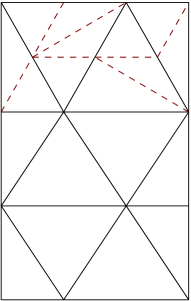
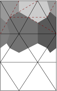
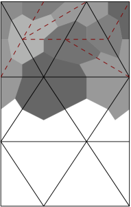
Next, we note that the discrete ansatz spaces are nested, while the discrete test spaces are not. However, in the non-refined area ${\mathcal{T}}_{\diamond}\cap{\mathcal{T}}_{\times}$ the shape of the dual grid elements is the same. We use this to truncate the sum of (60). To get the final sum over ${\mathcal{R}}_{\diamond}$ in (50), we have to define the functions $v_{\times}^{*}$ and $v^{*}_{\diamond}$ appropriately to apply Lemma 13 and Lemma 17, respectively. To formalize this, we define ${\mathcal{R}}^{*}_{\diamond}:={\mathcal{T}}^{*}_{\diamond}\backslash{\mathcal{T}}^{*}_{\times}$ and ${\mathcal{R}}^{*}_{\times}:={\mathcal{T}}^{*}_{\times}\backslash{\mathcal{T}}^{*}_{\diamond}$, i.e., the dual mesh of the refined areas; see Figure 4 for a 2D illustration. Note that

$$\bigcup_{V\in{\mathcal{R}}^{*}_{\diamond}}V=\bigcup_{V^{\prime}\in{\mathcal{R}}^{*}_{\times}}V^{\prime},$$ (61)

Consider the transition area ${\mathcal{R}}_{\diamond}\backslash({\mathcal{T}}_{\diamond}\backslash{\mathcal{T}}_{\times})=\big{\{}T\in{\mathcal{T}}_{\diamond}\cap{\mathcal{T}}_{\times}\,:\,\exists T^{\prime}\in{\mathcal{T}}_{\diamond}\backslash{\mathcal{T}}_{\times}\quad T\textasciimacron\cap T^{\prime}\neq\emptyset\big{\}}$ (second row of triangles in Figure 4) which consists of all non-refined neighbors of a refined element. For all $T\in{\mathcal{R}}_{\diamond}\backslash({\mathcal{T}}_{\diamond}\backslash{\mathcal{T}}_{\times})$, it holds

$$\big{\{}V\cap T\,:\,V\in{\mathcal{R}}^{*}_{\diamond}\big{\}}=\big{\{}V\cap T\,:\,V\in{\mathcal{R}}_{\times}^{*}\big{\}},$$

i.e., the shape of $V\in{\mathcal{R}}^{*}_{\diamond}$ coincides with the shape of some $V^{\prime}\in{\mathcal{R}}^{*}_{\times}$ in the transition area.

Let $v_{\times}:=u_{\times}-u_{\diamond}\in\SS^{1}_{0}({\mathcal{T}}_{\times})$. Choose $v_{\times}^{*}:={\mathcal{I}}_{\times}^{*}v_{\times}\in{\mathcal{P}}^{0}_{0}({\mathcal{T}}_{\times}^{*})$. Define $v^{*}_{\diamond}\in{\mathcal{P}}^{0}_{0}({\mathcal{T}}^{*}_{\diamond})$ by

$$v^{*}_{\diamond}|_{V}:=\begin{cases}(\Pi^{*}_{\diamond}v_{\times})|_{V}\quad&\text{if }V\in{\mathcal{R}}^{*}_{\diamond},\\ ({\mathcal{I}}^{*}_{\diamond}v_{\times})|_{V}\quad&\text{otherwise}.\end{cases}$$

For $V\in{\mathcal{T}}^{*}_{\diamond}\backslash{\mathcal{R}}^{*}_{\diamond}={\mathcal{T}}^{*}_{\diamond}\cap{\mathcal{T}}_{\times}^{*}$, this implies $v^{*}_{\times}|_{V}=v^{*}_{\diamond}|_{V}$, i.e., $v^{*}_{\times}=v^{*}_{\diamond}$ within the white area of Figure 44(b) and 44(c). We use this observation to truncate the sum over ${\mathcal{T}}^{*}_{\diamond}$ in (60) and replace ${\mathcal{T}}^{*}_{\diamond}$ by ${\mathcal{R}}^{*}_{\diamond}$. Together with (45) from Lemma 14 for the bilinear forms, we get

$$\begin{split}{\mathcal{A}}(u_{\times}-u_{\diamond},v_{\times})&\leq C_{\rm bil}\sum_{T\in{\mathcal{T}}_{\times}}h_{T}\,|||u_{\times}-u_{\diamond}|||_{T}|||v_{\times}|||_{T}\\ &\quad+\sum_{V\in{\mathcal{R}}^{*}_{\diamond}}\Big{(}(R_{\diamond}\hskip 1.42262pt,v^{*}_{\times}-v^{*}_{\diamond})_{V}-\sum_{\zeta\in{\mathcal{F}}_{V,\diamond}}(J_{\diamond}\hskip 1.42262pt,v^{*}_{\times}-v^{*}_{\diamond})_{\zeta\backslash\Gamma}\Big{)}.\end{split}$$ (62)

Next, we estimate the sum over $T\in{\mathcal{T}}_{\times}$ by the Cauchy-Schwarz inequality. Furthermore, we add $v_{\times}-v_{\times}$ and use (61) to rewrite the sum over the boxes $V\in{\mathcal{R}}^{*}_{\diamond}$ in (62):

$$\begin{split}{\mathcal{A}}(u_{\times}-u_{\diamond},v_{\times})&\leq\Big{(}\sum_{T\in{\mathcal{T}}_{\times}}h_{T}^{2}\,|||u_{\times}-u_{\diamond}|||_{T}^{2}\Big{)}^{1/2}\,|||v_{\times}|||\\ &\qquad+\sum_{V\in{\mathcal{R}}^{*}_{\diamond}}\Big{(}(R_{\diamond}\hskip 1.42262pt,v_{\times}-v^{*}_{\diamond})_{V}-\sum_{\zeta\in{\mathcal{F}}_{V,\diamond}}(J_{\diamond}\hskip 1.42262pt,v_{\times}-v^{*}_{\diamond})_{\zeta\backslash\Gamma}\Big{)}\\ &\qquad+\sum_{V^{\prime}\in{\mathcal{R}}^{*}_{\times}}\Big{(}(R_{\diamond}\hskip 1.42262pt,v^{*}_{\times}-v_{\times})_{V^{\prime}}-\sum_{\zeta^{\prime}\in{\mathcal{F}}_{V^{\prime},\times}\atop\zeta^{\prime}\subset F\in{\mathcal{F}}_{\diamond}}(J_{\diamond}\hskip 1.42262pt,v^{*}_{\times}-v_{\times})_{\zeta^{\prime}\backslash\Gamma}\Big{)}.\end{split}$$ (63)

Note that ${\mathcal{F}}_{V^{\prime},\times}$ contains also parts of facets from ${\mathcal{T}}_{\times}$ which are not needed here and which are avoided by $\zeta^{\prime}\subset F\in{\mathcal{F}}_{\diamond}$. To abbreviate notation, let $h_{V}:={\rm diam}(V)$ and note that $\sigma$-shape regularity implies $h_{V}\simeq h_{T}$ for all $V\in{\mathcal{T}}^{*}_{\diamond}$ and $T\in{\mathcal{T}}_{\diamond}$ with $V\cap T\neq\emptyset$. Next, we estimate the two sums over ${\mathcal{R}}^{*}_{\diamond}$ and ${\mathcal{R}}^{*}_{\times}$: First, with (58) and (59) of Lemma 17 and $v^{*}_{\diamond}|_{V}=\Pi^{*}_{\diamond}v_{\times}|_{V}$ for all $V\in{\mathcal{R}}^{*}_{\diamond}$, the Cauchy-Schwarz inequality yields

$$\sum_{V\in{\mathcal{R}}^{*}_{\diamond}}\Big{(}(R_{\diamond}\hskip 1.42262pt,v_{\times}-v^{*}_{\diamond})_{V}-\sum_{\zeta\in{\mathcal{F}}_{V,\diamond}}(J_{\diamond}\hskip 1.42262pt,v_{\times}-v^{*}_{\diamond})_{\zeta\backslash\Gamma}\Big{)}$$

$$\quad\lesssim\bigg{[}\Big{(}\sum_{V\in{\mathcal{R}}^{*}_{\diamond}}h_{V}^{2}\|R_{\diamond}\|_{L^{2}(V)}^{2}\Big{)}^{1/2}+\Big{(}\sum_{V\in{\mathcal{R}}^{*}_{\diamond}}\sum_{\zeta\in{\mathcal{F}}_{V,\diamond}}h_{V}\|J_{\diamond}\|_{L^{2}(\zeta\backslash\Gamma)}^{2}\Big{)}^{1/2}\bigg{]}\,\Big{(}\sum_{V\in{\mathcal{R}}^{*}_{\diamond}}\|\nabla v_{\times}\|_{L^{2}(V)}^{2}\Big{)}^{1/2}.$$

With $$\bigcup_{V\in{\mathcal{R}}^{*}_{\diamond}}V\subset\bigcup_{T\in{\mathcal{R}}_{\diamond}}T$$, we hence obtain

$$\quad\lesssim\bigg{[}\sum_{T\in{\mathcal{R}}_{\diamond}}\big{(}h_{T}^{2}\,\|R_{\diamond}\|_{L^{2}(T)}^{2}+h_{T}\,\|J_{\diamond}\|_{L^{2}(\partial T\backslash\Gamma)}^{2}\big{)}\bigg{]}^{1/2}\,|||v_{\times}|||=\Big{(}\sum_{T\in{\mathcal{R}}_{\diamond}}\eta_{\diamond}(T)^{2}\Big{)}^{1/2}\,|||v_{\times}|||.$$ (64)

Note that $\bigcup_{V^{\prime}\in{\mathcal{R}}^{*}_{\times}}V^{\prime}\subset\bigcup_{T\in{\mathcal{R}}_{\diamond}}T$. Then, with (43) and (44) of Lemma 13 and $v_{\times}^{*}={\mathcal{I}}_{\times}v_{\times}$, we get as before

$$\sum_{V^{\prime}\in{\mathcal{R}}^{*}_{\times}}\Big{(}(R_{\diamond}\hskip 1.42262pt,v^{*}_{\times}-v_{\times})_{V^{\prime}}-\sum_{\zeta^{\prime}\in{\mathcal{F}}_{V^{\prime},\times}\atop\zeta^{\prime}\subset F\in{\mathcal{F}}_{\diamond}}(J_{\diamond}\hskip 1.42262pt,v^{*}_{\times}-v_{\times})_{\zeta^{\prime}\backslash\Gamma}\Big{)}$$

$$\quad\lesssim\bigg{[}\sum_{T\in{\mathcal{R}}_{\diamond}}\big{(}h_{T}^{2}\,\|R_{\diamond}\|_{L^{2}(T)}^{2}+h_{T}\,\|J_{\diamond}\|_{L^{2}(\partial T\backslash\Gamma)}^{2}\big{)}\bigg{]}^{1/2}\,|||v_{\times}|||=\Big{(}\sum_{T\in{\mathcal{R}}_{\diamond}}\eta_{\diamond}(T)^{2}\Big{)}^{1/2}\,|||v_{\times}|||.$$ (65)

Combining (3.8)–(3.8) with (63), we obtain

$${\mathcal{A}}(u_{\times}-u_{\diamond},v_{\times})\lesssim\bigg{[}\Big{(}\sum_{T\in{\mathcal{T}}_{\times}}h_{T}^{2}\,|||u_{\times}-u_{\diamond}|||_{T}^{2}\Big{)}^{1/2}+\Big{(}\sum_{T\in{\mathcal{R}}_{\diamond}}\eta_{\diamond}(T)^{2}\Big{)}^{1/2}\bigg{]}\,|||v_{\times}|||.$$

Finally, ellipticity of ${\mathcal{A}}(\cdot,\cdot)$ and the choice of $v_{\times}=u_{\times}-u_{\diamond}$ show

$$|||u_{\times}-u_{\diamond}|||^{2}\lesssim{\mathcal{A}}(u_{\times}-u_{\diamond},v_{\times})\lesssim\bigg{[}\sum_{T\in{\mathcal{T}}_{\times}}h_{T}^{2}\,|||u_{\times}-u_{\diamond}|||_{T}^{2}+\sum_{T\in{\mathcal{R}}_{\diamond}}\eta_{\diamond}(T)^{2}\bigg{]}^{1/2}\,|||u_{\times}-u_{\diamond}|||.$$

This proves (50) and concludes the proof. ∎

3.9. Proof of Theorem 7

Suppose that the initial triangulation ${\mathcal{T}}_{0}$ is sufficiently fine such that the following assumptions (i)–(iii) are satisfied:

• For all ${\mathcal{T}}_{\times}\in{\tt refine}({\mathcal{T}}_{0})$, the FVM system (13) is well-posed. In particular, Lemma 9 proves that stability (A1) and reduction (A2) are satisfied.

• Proposition 11 is valid and, in particular, the general quasi-orthogonality (A3) is satisfied.

• The constant $C_{\rm bil}$ from Proposition 15 satisfies $C_{\rm bil}\|h_{0}\|_{L^{\infty}(\Omega)}\leq 1/2$, so that Proposition 15, in fact, proves the discrete reliability (A4).

Finally, let $\widetilde{\mathcal{M}}_{\ell}\subseteq{\mathcal{T}}_{\ell}$ be a set of minimal cardinality which satisfies the Dörfler marking (30) for the error estimator. Then, the additional assumption of Theorem 7 (ii) and the choice of the marked elements ${\mathcal{M}}_{\ell}^{\eta}\subseteq{\mathcal{M}}_{\ell}\subseteq{\mathcal{T}}_{\ell}$ in Algorithm 4 imply that $\#{\mathcal{M}}_{\ell}\leq C_{\rm MNS}\,\#{\mathcal{M}}_{\ell}^{\eta}\leq C_{\rm MNS}C_{\rm mark}\,\#\widetilde{\mathcal{M}}_{\ell}$. Altogether, the assumptions of [CFPP14, Theorem 4.1] are fulfilled, and (32)–(33) follow for our adaptive FVM of Algorithm 4.∎

(a) ${\mathcal{T}}_{0}$ (16 elements).

(b) ${\mathcal{T}}_{8}$ (216 elements).

(c) ${\mathcal{T}}_{16}$ (3838 elements).

(d) Solution (${\mathcal{T}}_{16}$).

Figure 5. Experiment with smooth solution from Section 4.1: Initial triangulation ${\mathcal{T}}_{0}$ with NVB reference edges as well as adaptively generated meshes ${\mathcal{T}}_{8}$ resp. ${\mathcal{T}}_{16}$, and discrete FVM solution calculated on ${\mathcal{T}}_{16}$.

\psfragscanon\psfrag{s12}[l][l]{\scriptsize$1$}\psfrag{s04}[l][l]{\small$\eta_{\ell}$ (uni.)}\psfrag{s08}[l][l]{\small${\rm osc}_{\ell}$ (ada.)}\psfrag{s14}[l][l]{\scriptsize$1$}\psfrag{s05}[l][l]{\small$E_{\ell}$ (uni.)}\psfrag{s07}[l][l]{\small$\eta_{\ell}$ (ada.)}\psfrag{s01}[l][l]{\small${\rm osc}_{\ell}$ (uni.)}\psfrag{s02}[l][l]{\small$E_{\ell}$ (ada.)}\psfrag{s09}[l][l]{\scriptsize$1$}\psfrag{s10}[l][l]{\scriptsize$\;1/2$}\psfrag{s06}[t][t]{\small number of elements}\psfrag{s11}[b][b]{\small error, estimator, oscillation}\psfrag{x01}[t][t]{\scriptsize${10^{1}}$}\psfrag{x02}[t][t]{\scriptsize${10^{2}}$}\psfrag{x03}[t][t]{\scriptsize${10^{3}}$}\psfrag{x04}[t][t]{\scriptsize${10^{4}}$}\psfrag{x05}[t][t]{\scriptsize${10^{5}}$}\psfrag{x06}[t][t]{\scriptsize${10^{6}}$}\psfrag{x07}[t][t]{\scriptsize${10^{7}}$}\psfrag{v01}[r][r]{\scriptsize${10^{-3}}$}\psfrag{v02}[r][r]{\scriptsize${10^{-2}}$}\psfrag{v03}[r][r]{\scriptsize${10^{-1}}$}\psfrag{v04}[r][r]{\scriptsize${10^{0}}$}\psfrag{v05}[r][r]{\scriptsize${10^{1}}$}\psfrag{v06}[r][r]{\scriptsize${10^{2}}$}\psfrag{v07}[r][r]{\scriptsize${10^{3}}$}\includegraphics[width=346.89731pt]{figuresnumerics/bsp1-error.eps}

Figure 6. Experiment with smooth solution from Section 4.1: Error in the energy norm $E_{\ell}:=|||u-u_{\ell}|||$, weighted-residual error estimator $\eta_{\ell}$, and data oscillations ${\rm osc}_{\ell}$ for uniform and adaptive mesh-refinement.

(a) ${\mathcal{T}}_{0}$ (12 elements).

(b) ${\mathcal{T}}_{8}$ (204 elements).

(c) ${\mathcal{T}}_{16}$ (2451 elements).

(d) Solution (${\mathcal{T}}_{16}$).

Figure 7. Experiment with singular solution from Section 4.2: Initial triangulation ${\mathcal{T}}_{0}$ with NVB reference edges as well as adaptively generated meshes ${\mathcal{T}}_{8}$ resp. ${\mathcal{T}}_{16}$, and discrete FVM solution calculated on ${\mathcal{T}}_{16}$.

\psfragscanon\psfrag{s14}[l][l]{\small${\rm osc}_{\ell}$ (uni.)}\psfrag{s02}[t][t]{\small number of elements}\psfrag{s06}[l][l]{\small$E_{\ell}$ (uni.)}\psfrag{s08}[l][l]{\small$\eta_{\ell}$ (uni.)}\psfrag{s12}[l][l]{\small$E_{\ell}$ (ada.)}\psfrag{s03}[b][b]{\small error, estimator, oscillation}\psfrag{s09}[l][l]{\scriptsize$1/2$}\psfrag{s15}[l][l]{\small${\rm osc}_{\ell}$ (ada.)}\psfrag{s01}[l][l]{\scriptsize$1$}\psfrag{s10}[l][l]{\scriptsize$1$}\psfrag{s13}[l][l]{\scriptsize$\;1/3$}\psfrag{s11}[l][l]{\small$\eta_{\ell}$ (ada.)}\psfrag{s16}[l][l]{\scriptsize$1$}\psfrag{s05}[l][l]{\scriptsize$1$}\psfrag{x01}[t][t]{\scriptsize${10^{1}}$}\psfrag{x02}[t][t]{\scriptsize${10^{2}}$}\psfrag{x03}[t][t]{\scriptsize${10^{3}}$}\psfrag{x04}[t][t]{\scriptsize${10^{4}}$}\psfrag{x05}[t][t]{\scriptsize${10^{5}}$}\psfrag{x06}[t][t]{\scriptsize${10^{6}}$}\psfrag{x07}[t][t]{\scriptsize${10^{7}}$}\psfrag{v01}[r][r]{\scriptsize${10^{-6}}$}\psfrag{v02}[r][r]{\scriptsize${10^{-5}}$}\psfrag{v03}[r][r]{\scriptsize${10^{-4}}$}\psfrag{v04}[r][r]{\scriptsize${10^{-3}}$}\psfrag{v05}[r][r]{\scriptsize${10^{-2}}$}\psfrag{v06}[r][r]{\scriptsize${10^{-1}}$}\psfrag{v07}[r][r]{\scriptsize${10^{0}}$}\psfrag{v08}[r][r]{\scriptsize${10^{1}}$}\includegraphics[width=346.89731pt]{figuresnumerics/bsp2-error.eps}

Figure 8. Experiment with smooth solution from Section 4.2: Error in the energy norm $E_{\ell}:=|||u-u_{\ell}|||$, weighted-residual error estimator $\eta_{\ell}$, and data oscillations ${\rm osc}_{\ell}$ for uniform and adaptive mesh-refinement.

4. Numerical experiments

In this section, we illustrate the performance of Algorithm 4 with $\theta=0.5=\theta^{\prime}$ for two examples. In extension of our theory, we consider the model problem (6) with inhomogeneous Dirichlet boundary conditions. The numerical experiments are conducted in Matlab on a standard laptop with a dual core $2.8$ GHz processor and $16$ GB memory.

4.1. Experiment with smooth solution

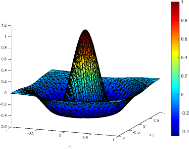
On the square $\Omega=(-1,1)^{2}$, we prescribe the exact solution $u(x_{1},x_{2})=(1-10x_{1}^{2}-10x_{2}^{2})e^{-5(x_{1}^{2}+x_{2}^{2})}$ with $x=(x_{1},x_{2})\in{\mathbb{R}}^{2}$. We choose the diffusion matrix

$$\mathbf{A}=\left(\begin{array}[]{rr}10+\cos x_{1}&9\,x_{1}x_{2}\\ 9\,x_{1}x_{2}&\;10+\sin x_{2}\end{array}\right),$$

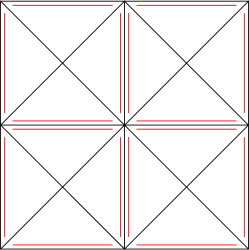
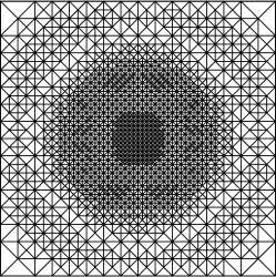
so that (7) holds with $\lambda_{\min}=0.82293$ and $\lambda_{\max}=10.84096$. The right-hand side $f$ is calculated appropriately. The uniform initial mesh ${\mathcal{T}}^{(0)}$ consists of $16$ triangles; see Figure 57(a). In Figure 55(b) and 55(c) we see an adaptively generated mesh after $8$ and $16$ refinements, respectively. Figure 55(d) plots the smooth solution on the mesh ${\mathcal{T}}_{16}$. As $u$ is smooth, uniform and adaptive mesh-refinement lead to the optimal convergence order ${\mathcal{O}}(N^{-1/2})$ with respect to the number $N$ of elements; see Figure 6. The oscillations are of higher order and decrease with ${\mathcal{O}}(N^{-1})$. Table 19(a) shows the experimental validation of the additional assumption in Theorem 7 (ii) that marking for the data oscillations is negligible.

4.2. Experiment with generic singularity

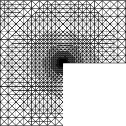
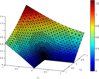
On the L-shaped domain $\Omega=\linebreak(-1,1)^{2}\backslash\big{(}[0,1]\times[-1,0]\big{)}$, we prescribe the exact solution $u(x_{1},x_{2})=r^{2/3}\sin(2\varphi/3)$ in polar coordinates $r\in{\mathbb{R}}_{0}^{+}$, $\varphi\in[0,2\pi[$, and $(x_{1},x_{2})=r(\cos\varphi,\sin\varphi)$. Then, $u$ has a generic singularity at the reentrant corner $(0,0)$, which leads to $u\in H^{1+2/3-\varepsilon}(\Omega)$ for all $\varepsilon>0$. We choose the diffusion matrix

$$\mathbf{A}=\left(\begin{array}[]{rr}5+(x_{1}^{2}+x_{2}^{2})\cos x_{1}&(x_{1}^{2}+x_{2}^{2})^{2}\\ (x_{1}^{2}+x_{2}^{2})^{2}&\;5+(x_{1}^{2}+x_{2}^{2})\sin x_{2}\end{array}\right)$$

so that (7) holds with $\lambda_{\min}=0.46689$ and $\lambda_{\max}=5.14751$. The right-hand side $f$ is calculated appropriately. The uniform initial mesh ${\mathcal{T}}^{(0)}$ consists of $12$ triangles. Some further adaptively generated meshes together with a plot of the discrete solution are shown in Figure 7.

For uniform mesh refinement, we observe the expected suboptimal convergence order of ${\mathcal{O}}(N^{-1/3})$, while adaptive mesh-refinement regains the optimal convergence order of ${\mathcal{O}}(N^{-1/2})$; see Figure 8. As in the experiment of Section 4.1, the oscillations are of higher order ${\mathcal{O}}(N^{-1})$. See Table 19(b) for the experimental validation of the additional assumption in Theorem 7 (ii) that marking for the data oscillations is negligible.

$\ell$	$\#{\mathcal{T}}_{\ell}$	$\#{\mathcal{M}}_{\ell}/\#{\mathcal{M}}_{\ell}^{\eta}$	${\rm osc}({\mathcal{M}}_{\ell}^{\eta})^{2}/{\rm osc}_{\ell}^{2}$
0	16	1.000	0.634
1	22	1.000	0.613
2	28	1.000	0.704
3	32	1.000	0.769
4	40	1.214	0.338
5	78	1.111	0.449
6	112	1.133	0.292
7	156	1.119	0.410
8	216	1.062	0.393
9	331	1.198	0.263
10	460	1.014	0.474
11	660	1.049	0.371
12	944	1.027	0.430
13	1,340	1.025	0.404
14	1,914	1.019	0.383
15	2,752	1.026	0.374
16	3,838	1.015	0.358
17	5,428	1.003	0.449
18	7,430	1.013	0.359
19	10,572	1.003	0.445
20	14,462	1.019	0.322
21	20,264	1.004	0.431
22	27,532	1.004	0.455
23	38,402	1.010	0.323
24	52,366	1.000	0.539
25	72,386	1.007	0.401
26	98,144	1.000	0.509
27	135,076	1.004	0.445
28	184,006	1.000	0.605
29	251,668	1.002	0.475
30	341,940	1.001	0.488
31	461,354	1.000	0.616
32	634,922	1.004	0.415
33	852,264	1.000	0.663
34	1,171,426	1.002	0.465
35	1,567,542	1.000	0.611
36	2,150,232	1.000	0.521
37	2,893,626	1.000	0.652
38	3,932,562	1.000	0.593
39	5,335,740	1.000	0.493

(a) Section 4.1.

$\ell$	$\#{\mathcal{T}}_{\ell}$	$\#{\mathcal{M}}_{\ell}/\#{\mathcal{M}}_{\ell}^{\eta}$	${\rm osc}({\mathcal{M}}_{\ell}^{\eta})^{2}/{\rm osc}_{\ell}^{2}$
0	12	1.667	0.143
1	18	1.750	0.115
2	26	1.400	0.108
3	35	1.222	0.062
4	56	1.200	0.104
5	78	1.643	0.028
6	110	1.350	0.135
7	148	1.161	0.290
8	204	1.111	0.268
9	274	1.048	0.423
10	370	1.168	0.223
11	525	1.069	0.324
12	704	1.063	0.296
13	961	1.015	0.442
14	1,314	1.003	0.475
15	1,784	1.037	0.345
16	2,451	1.000	0.639
17	3,305	1.015	0.417
18	4,562	1.000	0.595
19	6,161	1.001	0.482
20	8,344	1.011	0.440
21	11,316	1.000	0.635
22	15,249	1.000	0.528
23	20,631	1.000	0.577
24	27,742	1.014	0.451
25	37,566	1.000	0.655
26	50,139	1.011	0.437
27	67,722	1.000	0.571
28	90,543	1.000	0.523
29	121,136	1.005	0.471
30	163,221	1.000	0.715
31	216,681	1.025	0.361
32	292,527	1.000	0.545
33	389,411	1.000	0.582
34	521,975	1.013	0.437
35	699,195	1.000	0.678
36	928,417	1.012	0.418
37	1,246,972	1.000	0.561
38	1,658,877	1.000	0.585
39	2,224,754	1.003	0.481
40	2,959,035	1.000	0.659

(b) Section 4.2.

Table 1. Experimental results on marking strategy: We compute $\widetilde{C}_{MNS}:=\#{\mathcal{M}}_{\ell}/\#{\mathcal{M}}_{\ell}^{\eta}\leq 2$ and see that the additional assumption in Theorem 7 (ii) is experimentally verified. In addition, we compute $\widetilde{\theta}^{\prime}:={\rm osc}_{\ell}({\mathcal{M}}_{\ell}^{\eta})^{2}/{\rm osc}_{\ell}^{2}\geq 0.02$, i.e., the choice $\theta=0.5$, $\theta^{\prime}=0.02$ would guarantee ${\mathcal{M}}_{\ell}={\mathcal{M}}_{\ell}^{\eta}$ in Algorithm 4.

References

- [AO00] M. Ainsworth and J. T. Oden. A posteriori error estimation in finite element analysis. Pure and Applied Mathematics (New York). Wiley-Interscience [John Wiley & Sons], New York, 2000.
- [BDD04] P. Binev, W. Dahmen, and R. DeVore. Adaptive finite element methods with convergence rates. Numer. Math., 97(2):219–268, 2004.
- [BR87] R. E. Bank and D. J. Rose. Some error estimates for the box method. SIAM J. Numer. Anal., 24(4):777–787, 1987.
- [Cai91] Z. Cai. On the finite volume element method. Numer. Math., 58(7):713–735, 1991.
- [CFPP14] C. Carstensen, M. Feischl, M. Page, and D. Praetorius. Axioms of adaptivity. Comput. Math. Appl., 67:1195–1253, 2014.
- [Cha02] P. Chatzipantelidis. Finite volume methods for elliptic PDEs: a new approach. M2AN Math. Model. Numer. Anal., 36(2):307–324, 2002.
- [CKNS08] J. M. Cascon, C. Kreuzer, R. H. Nochetto, and K. G. Siebert. Quasi-optimal convergence rate for an adaptive finite element method. SIAM J. Numer. Anal., 46(5):2524–2550, 2008.
- [CKPS15] C. Carstensen, K. Köhler, D. Peterseim, and M. Schedensack. Comparison results for the Stokes equations. Appl. Numer. Math., 95:118–129, 2015.
- [CLT05] C. Carstensen, R. D. Lazarov, and S. Z. Tomov. Explicit and averaging a posteriori error estimates for adaptive finite volume methods. SIAM J. Numer. Anal., 42(6):2496–2521, 2005.
- [CPS12] C. Carstensen, D. Peterseim, and M. Schedensack. Comparison results of finite element methods for the Poisson model problem. SIAM J. Numer. Anal., 50(6):2803–2823, 2012.
- [Dör96] W. Dörfler. A convergent adaptive algorithm for Poisson’s equation. SIAM J. Numer. Anal., 33(3):1106–1124, 1996.
- [DS80] T. Dupont and R. Scott. Polynomial approximation of functions in Sobolev spaces. Math. Comp., 34(150):441–463, 1980.
- [EGH00] R. Eymard, T. Gallouët, and R. Herbin. Finite volume methods. In Handbook of numerical analysis, Vol. VII, pages 713–1020. North-Holland, Amsterdam, 2000.
- [ELL02] R. E. Ewing, T. Lin, and Y. Lin. On the accuracy of the finite volume element method based on piecewise linear polynomials. SIAM J. Numer. Anal., 39(6):1865–1888, 2002.
- [EP08] C. Erath and D. Praetorius. A posteriori error estimate and adaptive mesh refinement for the cell-centered finite volume method for elliptic boundary value problems. SIAM J. Numer. Anal., 47(1):109–135, 2008.
- [Era10] C. Erath. Coupling of the Finite Volume Method and the Boundary Element Method - Theory, Analysis, and Numerics. PhD thesis, University of Ulm, 2010.
- [Era12] C. Erath. Coupling of the finite volume element method and the boundary element method: an a priori convergence result. SIAM J. Numer. Anal., 50(2):574–594, 2012.
- [Era13] C. Erath. A posteriori error estimates and adaptive mesh refinement for the coupling of the finite volume method and the boundary element method. SIAM J. Numer. Anal., 51(3):1777–1804, 2013.
- [FFK+14] M. Feischl, T. Führer, M. Karkulik, J. M. Melenk, and D. Praetorius. Quasi-optimal convergence rates for adaptive boundary element methods with data approximation. Part I: Weakly-singular integral equation. Calcolo, 51(4):531–562, 2014.
- [FFK+15] M. Feischl, T. Führer, M. Karkulik, J. M. Melenk, and D. Praetorius. Quasi-optimal convergence rates for adaptive boundary element methods with data approximation. Part II: Hyper-singular integral equation. Electron. Trans. Numer. Anal., 44:153–176, 2015.
- [FFP14] M. Feischl, T. Führer, and D. Praetorius. Adaptive FEM with optimal convergence rates for a certain class of nonsymmetric and possibly nonlinear problems. SIAM J. Numer. Anal., 52(2):601–625, 2014.
- [FKMP13] M. Feischl, M. Karkulik, J. M. Melenk, and D. Praetorius. Quasi-optimal convergence rate for an adaptive boundary element method. SIAM J. Numer. Anal., 51(2):1327–1348, 2013.
- [Gan13] T. Gantumur. Adaptive boundary element methods with convergence rates. Numer. Math., 124(3):471–516, 2013.
- [Hac89] W. Hackbusch. On first and second order box schemes. Computing, 41(4):277–296, 1989.
- [KPP13] M. Karkulik, D. Pavlicek, and D. Praetorius. On 2D newest vertex bisection: optimality of mesh-closure and -stability of -projection. Constr. Approx., 38(2):213–234, 2013.
- [MNS00] P. Morin, R. H. Nochetto, and K. G. Siebert. Data oscillation and convergence of adaptive FEM. SIAM J. Numer. Anal., 38(2):466–488, 2000.
- [Nic05] S. Nicaise. A posteriori error estimations of some cell-centered finite volume methods. SIAM J. Numer. Anal., 43(4):1481–1503, 2005.
- [Ste07] R. Stevenson. Optimality of a standard adaptive finite element method. Found. Comput. Math., 7(2):245–269, 2007.
- [Ste08] R. Stevenson. The completion of locally refined simplicial partitions created by bisection. Math. Comp., 77(261):227–241, 2008.
- [Ver13] R. Verfürth. A posteriori error estimation techniques for finite element methods. Numerical Mathematics and Scientific Computation. Oxford University Press, Oxford, 2013.
- [Voh08] M. Vohralík. Residual flux-based a posteriori error estimates for finite volume and related locally conservative methods. Numer. Math., 111(1):121–158, 2008.
- [XZ06] J. Xu and Q. Zhu, Y.and Zou. New adaptive finite volume methods and convergence analysis. Preprint, Pennsylvania State University, 2006.
- [Zou10] Q. Zou. Hierarchical error estimates for finite volume approximation solution of elliptic equations. Appl. Numer. Math., 60(1-2):142–153, 2010.