∎
Tel.: +39 011 6706737, Fax: +39 011 751603
22email: rossella.cancelliere@unito.it 33institutetext: M. Gai 44institutetext: National Institute of Astrophysics, Astrophysical Observatory of Torino, Turin, Italy 55institutetext: P. Gallinari 66institutetext: Laboratory of Computer Sciences, LIP6, Université Pierre et Marie Curie, Paris, France
An analysis of numerical issues in neural training by pseudoinversion
Abstract
Some novel strategies have recently been proposed for single hidden layer neural network training that set randomly the weights from input to hidden layer, while weights from hidden to output layer are analytically determined by pseudoinversion. These techniques are gaining popularity in spite of their known numerical issues when singular and/or almost singular matrices are involved. In this paper we discuss a critical use of Singular Value Analysis for identification of these drawbacks and we propose an original use of regularisation to determine the output weights, based on the concept of critical hidden layer size. This approach also allows to limit the training computational effort. Besides, we introduce a novel technique which relies an effective determination of input weights to the hidden layer dimension. This approach is tested for both regression and classification tasks, resulting in a significant performance improvement with respect to alternative methods.
Keywords:
pseudoinverse matrix weights setting regularisation supervised learning1 Introduction
The training of one of the most common neural architecture, the single hidden layer feedforward neural network (SLFN) was mainly accomplished in past decades by methods based on gradient descent, and among them the large family of techniques based on backpropagation (Rumelhart et al., 1986). The start-up of these techniques assigns random values to the weights connecting input, hidden and output nodes that are then iteratively modified according to the error gradient steepest descent direction. Some common drawbacks with gradient descent-based learning are anyway the high computational cost because of slow convergence and the relevant risk of converging to poor local minima on the landscape of the error function (LeCun et al., 1998).
The idea of using the simple and efficient training algorithms of radial basis function neural networks, based on matricial pseudoinversion (Poggio and Girosi, 1990), also for SLFN learning was initially suggested in (Cancelliere, 2001); some appealing techniques were than developed (Nguyen et al., 2010; Kohno et al., 2010; Ajorloo et al., 2007) and among them the extreme learning machine ELM, (Huang et al., 2006) which has been successfully applied to a number of real-world applications (Sun et al., 2008; Wang et al., 2008; Malathi et al., 2010; Minhas et al., 2010), showing a good generalization performance with an extremely fast learning speed.
ELM main result states that SLFNs with randomly chosen input weights and hidden layer biases can learn distinct observations with a desired precision, provided that activation functions in the hidden layer are infinitely differentiable.
After input weights and hidden layer biases have been randomly set, output weights are directly evaluated by Moore-Penrose generalised inverse (or pseudoinverse) of the hidden layer output matrix: these two steps conclude one training phase and weights are no more modified, so that their determination is no more iterative in the sense of back-propagation based techniques.
Besides, all pseudoinversion based methods are multi-start, i.e. the above procedure is repeated meny times in order to find a good minimum of the error surface. Each training procedure so implies many random settings of input weights and as many evaluations of output weights through pseudoinversion.
However, such techniques seem to require more hidden units than typical values from backpropagation training to achieve comparable accuracy, as discussed in Yu and Deng (Yu and Deng, 2012). Moreover, pseudoinversion, commonly evaluated by Singular Value Decomposition (SVD), is a powerful method but some caution is required, since its numerical instability is a well known issue when singular and almost singular matrices are involved.
One aim of this paper is the analysis of these instability issues; a preliminary assessment of the context and our initial results are discussed in (Cancelliere et al., 2012). Here we present further advances on the theoretical framework and we propose a novel approach to carry out a more efficient learning, showing how singular values of SVD can be used to detect the occurrence of numerical instability.
Besides, we prove the existence of a critical hidden layer dimension that allows a careful tuning of the regularisation parameter and the use of regularisation to replace unstable, ill-posed problems with well-posed ones. We also propose an original method to set input weights that links their size to the hidden layer dimension and we show its effectiveness.
In section 2 we introduce the notation used for describing SLFN architectures, and the main ideas concerning input weights setting and output weights evaluation by pseudoinversion. In section 3 we discuss the problem of ill-posedness, and the basic regularisation concepts.
In section 4 our framework is tested on some applications selected from the UCI database. A substantial improvement in performance with respect to unregularised state-of-the-art techniques is shown.
2 Input and output weights determination
Fig. 1 shows a standard SLFN with input neurons, hidden neurons with non-linear activation functions , and output neurons with linear activation functions.
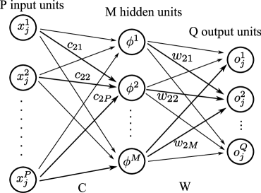
If we have a training set made by distinct training samples of (input, output) pairs , where and , the training aims at obtaining the matrix of desired outputs when the matrix of all input instances is presented as input.
We emphasise that, in the state of the art pseudoinverse approach, input weights (and hidden neurons biases) are randomly sampled from a uniform distribution in a fixed interval and no longer modified. Therefore this step gives the actual input weights values.
After having fixed the input weights matrix C, the use of linear output units allows to determine output weights as the solution of the linear system
| (1) |
where is the hidden layer output matrix of the neural network, . It is important to underline that because usually the number of hidden nodes is much lower than the number of distinct training samples, i.e. , is a rectangular matrix.
The least-squares solution of the linear system (1), as shown e.g. in (Penrose and Todd, 1956; Bishop, 2006), is where is the Moore-Penrose generalised inverse (or pseudoinverse) of matrix . It can be computed in a computationally simple and accurate way by using singular value decomposition (SVD) (Golub and Van Loan, 1996).
We know that every matrix can be decomposed as follows:
| (2) |
where and are orthogonal matrices and is a rectangular diagonal matrix whose elements , called singular values, are nonnegative (usually the singular values are listed in descending order, i.e. , = min , so that is uniquely determined).
The pseudoinverse matrix has the form
| (3) |
where is obtained from by taking the reciprocal of each non-zero element , and transposing the resulting matrix (Rao and Mitra, 1971). The presence of very small element is therefore a potential drawback of this method.
For computational reasons, the elements equal to zero or smaller than a predefined threshold are replaced by zeros (Golub and Van Loan, 1996).
3 Singular value decomposition of regularised problems
To turn an original ill-posed problem into a well-posed one, i.e. roughly speaking into a problem insensitive to small changes in training conditions, regularisation methods are often used (Badeva and Morozov, 1991), and Tikhonov regularisation is one of the most common (Tikhonov and Arsenin, 1977; Tikhonov, 1963).
The error functional to be minimised is characterized by a penalty term that depends from the so called Tikhonov matrix :
| (4) |
This matrix can for instance derive from the choice of using highpass operators (e.g. a difference operator or a weighted Fourier operator) to enforce smoothness.
The regularised solution, that we denote by , is now given by:
| (5) |
The penalty term improves on stability, making the problem less sensitive to initial conditions, and contains model complexity avoiding overfitting, as largely discussed in (Gallinari and Cibas, 1999).
To give preference to solutions with smaller norm (Bishop, 2006) a frequent choice is , so eqs. (4) and (5) can be rewritten as
| (6) |
| (7) |
The role of the control parameter is to trade off between the two error terms and . If , eq.(7) reduces to the unregularised least-squares solution, provided that exists.
The regularised solution (7) can also be expressed (see e.g. (Fuhry and Reichel, 2012)) as:
| (8) |
where are from the singular value decomposition of (eq.(2)) and is a rectangular diagonal matrix with elements
| (9) |
obtained using the singular values of .
It is evident that, when unregularised pseudoinversion is used, the presence of very small singular values can easily causes numerical instability in ; on the contrary, regularisation has a dramatic impact because, even in presence of very small values of the original unregularised problem, a careful choice of the parameter allows to tune singular values of the regularised matrix, preventing them from divergence.
It is clear at this point that a suitable value for the parameter has to derive from a compromise between the necessity to have it sufficiently large to control the approaching to zero of in eq.(9) while avoiding predominance of penalty term in eq.(6). Its tuning is therefore crucial to simultaneously control numerical instability and overfitting.
In the next section we propose a strategy to obtain this result showing that we achieve better performance and more stable solutions.
4 Experiments and Results
Some numerical instability issues have already been evidenced in our previous investigations (Cancelliere et al., 2012); we provided suggestions on possible mitigation techniques like selection of a convenient activation function and normalisation of the input weights. Hereafter we show that adding regularisation to the implementation prescriptions already analysed provides a convenient and effective approach to deal with such problem.
The use of sigmoidal activation functions has recently been subject of debate because they seem to be more easily driven towards saturation due to their non-zero mean value (Bengio and Glorot, 2010), while hyperbolic tangent seems less sensitive to this problem.
We select therefore both activation functions for a test aiming at comparing their performance in a context where we also compare our proposed regularised approach and the unregularised one. Four different experimental settings will be analysed, namely HypT-reg, Sigm-reg, HypT-unreg and Sigm-unreg.
| Dataset | Type | N. Instances | N. Attributes | N. Classes |
|---|---|---|---|---|
| Abalone | Regression | 4177 | 8 | - |
| Cpu | Regression | 209 | 6 | - |
| Delta Aileron | Regression | 7129 | 5 | - |
| Iris | Classification | 150 | 4 | 3 |
| Diabetes | Classification | 768 | 8 | 2 |
| Landsat | Classification | 4435 | 36 | 7 |
To further mitigate saturation issues, in our previous work (Cancelliere et al., 2012) we selected input weights according to a uniform random distribution in the range (, ), where is the number of hidden nodes. This links the size of input weights, and therefore of hidden neurons inputs, to the network architecture, thus forcing the use of the almost linear central part of the hyperbolic and sigmoidal activation functions when exploring the performance as a function of an increasing number of nodes. Such prescriptions are retained in the current work.
We emphasise that so doing input weights are automatically chosen ”small”, because the size of interval (, ) decreases when the number of hidden neurons increases: for instance with 10 hidden neurons, weights values are roughly selected in the range , with 100 hidden neurons in the range , and so on.
Because of the wide use among researchers belonging to ELM-community (see for instance (Helmy and Rasheed, 2009; Huang et al., 2006; Sun et al., 2008) our performance is also compared with that from unregularised pseudoinversion, input weights selected according to a random uniform distribution in the interval and sigmoidal activation functions (hereafter, ELM).
The numerical experiment compares these frameworks applying them to six benchmark datasets from the UCI repository (Bache and Lichman, 2013), listed in Table 1.
For each proposed method the number of hidden nodes is gradually increased by unity steps, and, for each selected size of SLFN, average RMSE or average misclassification rate on the validation set are computed over a set of 100 simulation trials, i.e. over 100 different initial choices of input weights. All simulations are carried out in Matlab 7.3 environment.
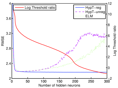
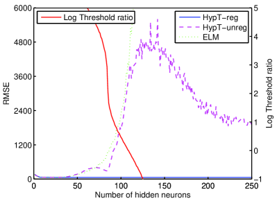
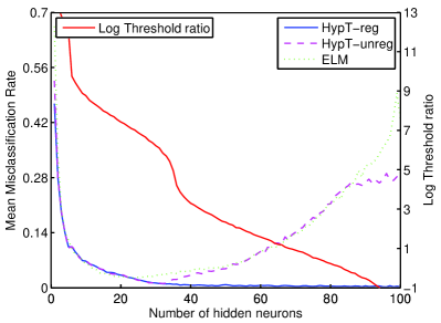
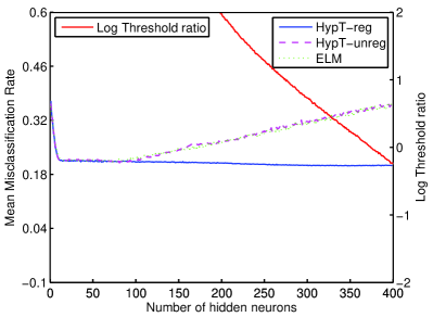
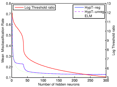
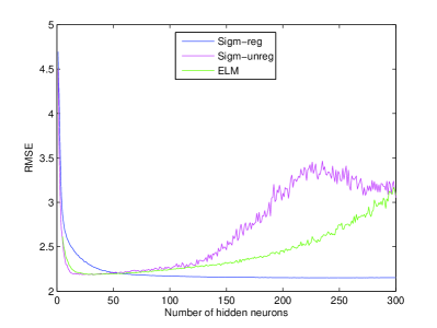
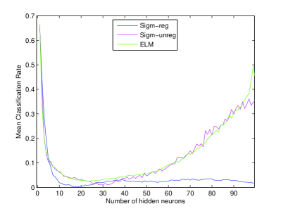
Figure 2 gives an insight on the performance trend (resp. average RMSE for regression or average misclassification rate for classification tasks) as a function of hidden space dimensionality for the cases HypT-reg, HypT-unreg and ELM. In Figure 3 performance trends are shown for the cases SigmT-reg, Sigm-unreg and, for the sake of comparison, again ELM; because of their similarity with the HypT cases, plots are shown for only two datasets (i.e. Abalone and Iris).
It is interesting to note that when unregularised techniques are used, all datasets except Landsat show a fast error growth; besides, the curves have different characteristics for HypT-unreg and Sigm-unreg on one side and ELM on the other, showing error peaks in the formers while monotonically increasing error values are obtained in the latter. We conjecture the presence of two distinct phenomena: numerical instability and overfitting.
In order to address the former issue, i.e. numerical instability, we evaluate for each dataset the ratio between the minimum singular value of hidden output matrix and the Matlab default threshold (below which singular values are considered too small and therefore treated as zero).
We checked that for each dataset processed with HypT-unreg or Sigm-unreg methods there is a critical hidden layer size above which the ratio becomes smaller than one; its trend is plotted in logarithmic units (red line, right scale), in Figure 2 for HypT-unreg case.
When approaching critical size, inversion of singular values causes a wrong evaluation of and therefore a significant growth in the error; when the critical dimension is reached, singular values under threshold are automatically removed, thus allowing the subsequent decrease of error. The same trend was detected analysing the astronomical dataset in (Cancelliere et al., 2012).
This decrease is anyway not sufficient to reach optimal error values because of overfitting, which is known to arise when a large amount of hidden neurons is available to reproduce almost exactly the training data.
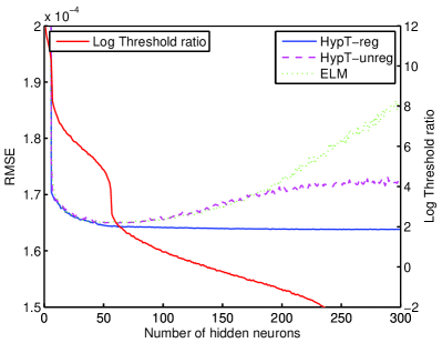
An even more severe overfitting affects ELM in fact in this case test error is a monotonically increasing function of the number of hidden neurons. A possible explanation is that the setting of input weights in the interval (-1, 1) may allow ‘specialisation’ of some hidden neurons on particular training instances, thus creating a sort of network partition, carried out thanks to saturation. On the contrary, when weights are randomly selected in the interval , as for HypT-unreg and Sigm-unreg cases, input weights are automatically kept small when the network size increases, thus exploiting the central part of both activation functions: consequently saturation is avoided (Cancelliere et al., 2012).
After clarification of the main issues affecting unregularised approaches, we now discuss the regularised one, derived according to eq.(8).
Looking at HypT-reg and Sigm-reg cases in Figures 2 and 3, it appears that not only numerical instability (i.e. the error peak) is removed, but also that the penalty term provides control of overfitting, avoiding error growth and allowing optimal exploitation of the superior potential of larger architectures. The error curves feature now a monotonic decrease, becoming increasingly smoother.
We obtained this result basing on the implications of eq.(9) that clearly suggests the role of the parameter in preventing instability: our original idea is to address the issue of its determination with an ‘ad hoc’ tuning whenever growing error drift is experienced by the unregularised approach, as follows.
We evaluate the validation error trend inside the critical region, looking for its minimum as a function of ; this allows to select a suitable value for this parameter for the subsequent experimentation with regularised pseudoinversion.
We then made 100 random input weight choices and evaluated the mean test error (RMSE or misclassification rate) and the standard deviation for any number of hidden neurons. In Table 2 we list for HypT-reg and Sigm-reg the best ones of these mean values, called Optimal performance, together with the number of hidden neurons used to reach the associated performance (in parenthesis), and the corresponding standard deviation, as well as the selected value of .
Error values significantly better, basing on the Student’s t-test evaluation of statistical confidence intervals, are recorded in bold. We can see that there is roughly no “winner” between HypT-reg and Sigm-reg.
Some other interesting considerations can be made noting that the regularised error plots in Figures 2 and 3, after an initial rapid decrease, achieve a nearly constant regime, with small variation vs. increasing numbers of hidden neurons. We can thus define a “near optimal” network size in both cases, as the one associated to a near optimal error level, i.e. an error significantly better than that from other methods. The assessment is again based on the Student’s t-test evaluation of statistical confidence intervals.
| Abalone | Cpu | Delta Ail. | |||||||
|---|---|---|---|---|---|---|---|---|---|
| RMSE | S | RMSE | S | RMSE | S | ||||
| HypT-reg | 2.168 (192) | 0.003 | 57.0 (78) | 2.1 | 1.639 (147) | 1.9e-3 | |||
| Sigm-reg | 2.150 (240) | 0.004 | 57.3 (88) | 1.8 | 1.636 (244) | 2.0e-3 | |||
| Iris | Diabetes | Landsat | |||||||
| Err.(%) | S(%) | Err.(%) | S(%) | Err.(%) | S(%) | ||||
| HypT-reg | (66) | 0.2 | (347) | 0.3 | 12.65 (486) | 0.2 | |||
| Sigm-reg | 0.2 (19) | 1.1 | 19.4 (95) | 0.6 | (396) | 0.3 |
| Abalone | Cpu | Delta Ail. | ||||
| RMSE | S | RMSE | S | RMSE | S | |
| HypT-reg (near opt.) | 2.181 (32) | 0.011 | 57.55 (22) | 6.2 | 1.642 (62) | 3.7e-3 |
| Sigm-reg (near opt.) | 2.181 (74) | 0.008 | 57.05 (45) | 3.2 | 1.647 (99) | 3.2e-3 |
| HypT-unreg | 2.187 (34) | 0.012 | 59.37 (17) | 7.2 | 1.649 (56) | 2.8e-4 |
| Sigm-unreg | 2.183 (32) | 0.013 | 57.58 (16) | 8.9 | 1.648 (45) | 6.5e-3 |
| ELM | 2.186 (33) | 0.015 | 59.48 (19) | 9.1 | 1.649 (75) | 8.8e-3 |
| Iris | Diabetes | Landsat | ||||
| Err.(%) | S(%) | Err.(%) | S(%) | Err.(%) | S(%) | |
| HypT-reg (near opt.) | 0.56 (37) | 0.9 | 21.0 (146) | 0.6 | 12.65 (486) | 0.2 |
| Sigm-reg (near opt.) | 0.3 (16) | 1.1 | 20.7 (45) | 0.8 | 13.77 (396) | 0.3 |
| HypT-unreg | 1.02 (30) | 1.1 | 21.2 (80) | 1.2 | 12.94 (295) | 0.4 |
| Sigm-unreg | 1.00 (29) | 1.2 | 20.8 (86) | 1.4 | 12.78 (377) | 0.4 |
| ELM | 2.52 (23) | 1.9 | 21.2 (69) | 1.2 | (390) | 0.4 |
Table 3 compares the performance of this near optimal network with those obtained with the other methods, listing the best mean error (with the associated number of hidden neurons in parenthesis) and the corresponding standard deviation.
Thus, it appears that regularisation provides, except for Landsat dataset, the best performance not only in terms of lowest error values (see table 2) but even with usage of smaller networks, limiting in this way computational cost and model complexity, and therefore fulfilling the goals set by previous researches (e.g. (Yu and Deng, 2012)). The smaller standard deviations almost always associated with the regularised methods also suggest a lower dependence from initial conditions.
We also highlight that the use of small input weights and sigmoidal activation functions, which characterizes the Sigm-unreg case, allows to obtain error values lower with respect to the ELM case, so confirming the effectiveness of this choice in order to contain saturation and overfitting issues.
Landsat dataset constitutes an exception because best performance is reached using ELM. In this case, regularisation does not seem to be required, because overfitting and/or numerical instability do not take place, as it appears from unregularised error curves. The behaviour of the threshold ratio, which remains always larger than unity, is consistent with the lack of numerical instability and with our hypothesis of its relationship with error peaks. The lack of overfitting appears to be specific to the complexity of the dataset, having input vectors with size much larger than others, and therefore requiring a significantly larger number of parameters.
In table 4 are listed the computational times (in seconds) recorded for all datasets for completing one training step, i.e. one random setting of input weights and one output weights evaluation through pseudoinversion of the hidden layer output matrix; the number of hidden neurons has been fixed to for the sake of comparison.
We can see that, for each dataset, the times associated to each method do not differ significantly, because after having fixed the number of hidden neurons, the computational load necessary for the processing is comparable.
The interested reader can find, for the common datatsets, a comparison among training times of ELM and backpropagation in (Huang et al., 2006), and can verify that ELM turns out to be two or three orders of magnitude faster.
| Abalone | Cpu | Delta Ail. | |
| HypT-reg | 0.032 | 0.035 | 0.093 |
| Sigm-reg | 0.029 | 0.040 | 0.096 |
| HypT-unreg | 0.018 | 0.018 | 0.064 |
| Sigm-unreg | 0.0151 | 0.025 | 0.077 |
| ELM | 0.0123 | 0.015 | 0.060 |
| Iris | Diabetes | Landsat | |
| HypT-reg | 0.037 | 0.0158 | 16.65 |
| Sigm-reg | 0.032 | 0.0155 | 16.77 |
| HypT-unreg | 0.017 | 0.0139 | 15.94 |
| Sigm-unreg | 0.021 | 0.0144 | 15.78 |
| ELM | 0.011 | 0.0116 | 14.32 |
5 Conclusions
We have considered the numerical instability ad overfitting problems for single hidden layer neural networks trained by pseudoinversion. We have shown how to use singular value analysis for the diagnosis of numerical instability, and how to solve this problem through the determination of a critical hidden layer region from which the regularisation technique benefits. This method also contributes to reduce the overfitting.
Tests have been performed for both regression and classification tasks. For five out of six cases, the proposed regularisation is proven necessary and provides a significant performance improvement with respect to unregularised techniques; it also allows to built lean architectures which achieve near optimal performance with a reduced number of hidden neurons.
Moreover the use of sigmoidal activation functions and “small” input weights (small because their values are linked to the hidden layer size), which characterizes the Sigm-unreg case, allows to obtain error values lower with respect to the ELM case, so confirming the effectiveness of this choice in order to contain saturation and overfitting issues.
Comparing our results on the common regression datasets with the alternative method proposed by Miche et al. (Miche et al., 2011), we note that our technique achieves RMSE values lower than those corresponding to their MSE values, with a somewhat lower number of neurons. Besides, in our opinion, our method is simpler, in the sense that it uses a single step of regularisation rather than two in their method, and we also deal with classification tasks.
6 Acknowledgment
The activity has been partially carried on in the context of the Visiting Professor Program of the Gruppo Nazionale per il Calcolo Scientifico (GNCS) of the Italian Istituto Nazionale di Alta Matematica (INdAM).
References
- Ajorloo et al. (2007) Ajorloo, H., Manzuri-Shalmani, M. T., and Lakdashti, A. (2007). Restoration of damaged slices in images using matrix pseudo inversion. In Proceedings of the 22nd International symposium on computer and information sciences.
- Bache and Lichman (2013) Bache, K. and Lichman, M. (2013). UCI machine learning repository.
- Badeva and Morozov (1991) Badeva, V. and Morozov, V. (1991). Problèmes incorrectement posés: Théorie et applications en identification , filtrage optimal, contrôle optimal, analyse et synthèse de systèmes, reconnaissance d’images. Série Automatique. Masson.
- Bengio and Glorot (2010) Bengio, Y. and Glorot, X. (2010). Understanding the difficulty of training deep feedforward neural networks. In Proceedings of AISTATS 2010, volume 9, pages 249–256.
- Bishop (2006) Bishop, C. M. (2006). Pattern Recognition and Machine Learning (Information Science and Statistics). Springer-Verlag New York, Inc., Secaucus, NJ, USA.
- Cancelliere (2001) Cancelliere, R. (2001). A high parallel procedure to initialize the output weights of a radial basis function or bp neural network. In Proceedings of the 5th International Workshop on Applied Parallel Computing, New Paradigms for HPC in Industry and Academia, PARA ’00, pages 384–390, London, UK, UK. Springer-Verlag.
- Cancelliere et al. (2012) Cancelliere, R., Gai, M., Artières, T., and Gallinari, P. (2012). Matrix pseudoinversion for image neural processing. In T. Huang, Z. Zeng, C. Li, and C. Leung, editors, Neural Information Processing, volume 7667 of Lecture Notes in Computer Science, pages 116–125. Springer Berlin Heidelberg.
- Fuhry and Reichel (2012) Fuhry, M. and Reichel, L. (2012). A new tikhonov regularization method. Numerical Algorithms, 59(3), 433–445.
- Gallinari and Cibas (1999) Gallinari, P. and Cibas, T. (1999). Practical complexity control in multilayer perceptrons. Signal Processing, 74, 29–46.
- Golub and Van Loan (1996) Golub, G. H. and Van Loan, C. F. (1996). Matrix computations (3rd ed.). Johns Hopkins University Press, Baltimore, MD, USA.
- Helmy and Rasheed (2009) Helmy, T. and Rasheed, Z. (2009). Multi-category bioinformatics dataset classification using extreme learning machine. In Proceedings of the Eleventh conference on Congress on Evolutionary Computation, CEC’09, pages 3234–3240, Piscataway, NJ, USA. IEEE Press.
- Huang et al. (2006) Huang, G.-B., Zhu, Q.-Y., and Siew, C.-K. (2006). Extreme learning machine: theory and applications. Neurocomputing, 70(1), 489–501.
- Kohno et al. (2010) Kohno, K., Kawamoto, M., and Inouye, Y. (2010). A matrix pseudoinversion lemma and its application to block-based adaptive blind deconvolution for mimo systems. Trans. Cir. Sys. Part I, 57(7), 1449–1462.
- LeCun et al. (1998) LeCun, Y., Bottou, L., Orr, G., and Müller, K.-R. (1998). Efficient backprop. pages 9–50. Springer Berlin Heidelberg.
- Malathi et al. (2010) Malathi, V., Marimuthu, N., and Baskar, S. (2010). Intelligent approaches using support vector machine and extreme learning machine for transmission line protection. Neurocomputing, 73(10–12), 2160 – 2167. Subspace Learning / Selected papers from the European Symposium on Time Series Prediction.
- Miche et al. (2011) Miche, Y., van Heeswijk, M., Bas, P., Simula, O., and Lendasse, A. (2011). Trop-elm: A double-regularized elm using lars and tikhonov regularization. Neurocomputing, 74(16), 2413 – 2421.
- Minhas et al. (2010) Minhas, R., Baradarani, A., Seifzadeh, S., and Wu, Q. J. (2010). Human action recognition using extreme learning machine based on visual vocabularies. Neurocomputing, 73(10–12), 1906 – 1917. Subspace Learning / Selected papers from the European Symposium on Time Series Prediction.
- Nguyen et al. (2010) Nguyen, T. D., Pham, H. T. B., and Dang, V. H. (2010). An efficient pseudo inverse matrix-based solution for secure auditing. In Proceedings of the IEEE International Conference on Computing and Communication Technologies, Research, Innovation, and Vision for the Future, IEEE International Conference.
- Penrose and Todd (1956) Penrose, R. and Todd, J. A. (1956). On best approximate solutions of linear matrix equations. Mathematical Proceedings of the Cambridge Philosophical Society, null, 17–19.
- Poggio and Girosi (1990) Poggio, T. and Girosi, F. (1990). Networks for approximation and learning. Proceedings of the IEEE, 78(9), 1481–1497.
- Rao and Mitra (1971) Rao, C. and Mitra, S. (1971). Generalized inverse of matrices and its applications. Wiley series in probability and mathematical statistics: Applied probability and statistics. Wiley.
- Rumelhart et al. (1986) Rumelhart, D. E., Hinton, G. E., and Williams, R. J. (1986). Parallel distributed processing: explorations in the microstructure of cognition, vol. 1. chapter Learning internal representations by error propagation, pages 318–362. MIT Press, Cambridge, MA, USA.
- Sun et al. (2008) Sun, Z.-L., Choi, T.-M., Au, K.-F., and Yu, Y. (2008). Sales forecasting using extreme learning machine with applications in fashion retailing. Decision Support Systems, 46(1), 411 – 419.
- Tikhonov and Arsenin (1977) Tikhonov, A. and Arsenin, V. (1977). Solutions of ill-posed problems. Scripta series in mathematics. Winston.
- Tikhonov (1963) Tikhonov, A. N. (1963). Solution of incorrectly formulated problems and the regularization method. Soviet Math. Dokl., 4, 1035–1038.
- Wang et al. (2008) Wang, G., Zhao, Y., and Wang, D. (2008). A protein secondary structure prediction framework based on the extreme learning machine. Neurocomputing, 72(1–3), 262 – 268. Machine Learning for Signal Processing (MLSP 2006) / Life System Modelling, Simulation, and Bio-inspired Computing (LSMS 2007).
- Yu and Deng (2012) Yu, D. and Deng, L. (2012). Efficient and effective algorithms for training single-hidden-layer neural networks. Pattern Recogn. Lett., 33(5), 554–558.