Robustness of Neutrino Mass Matrix Predictions

Abstract

We investigate the stability of neutrino mass matrix predictions on important and currently unknown observables. Those are the octant of $\theta_{23}$, the sign of $\sin\delta$ and the neutrino mass ordering. Determining those unknowns is expected to be useful in order to distinguish neutrino mass models. Therefore it may be interesting to know how robust the predictions of a mass matrix for the octant of $\theta_{23}$ or the neutrino mass ordering are. By applying general multiplicative perturbations we explicitly quantify how probable it is that a perturbed mass matrix predicts an octant of $\theta_{23}$ different from the original mass matrix, or even a neutrino mass ordering different from the original one. Both the general case and an explicit flavor symmetry model are studied. We give the probabilities as a function of the smallest neutrino mass, showing that for values exceeding 0.1 eV the chance to switch the prediction quickly approaches 50 %.

I Introduction

In recent years a consistent picture of lepton mixing has emerged Olive et al. (2014), with several parameters being determined with increasing precision (for a recent global fit of all existing data, see Ref. Capozzi et al. (2014)). A remarkable pattern has emerged, with one close-to-maximal mixing angle, one large and one small mixing angle, the latter being of the order of the largest quark mixing angle. While the overall picture of the leptonic mixing matrix is clear, comparable precision with respect to the quark sector is still lacking, but future experiments and facilities exist that will improve the errors on the parameters by remarkable amounts, see e.g. Balantekin et al. (2013). Of particular interest in neutrino physics are the octant of the atmospheric neutrino mixing angle $\theta_{23}$ and of course $\sin\delta$, the parameter governing leptonic CP violation. The mass ordering and the value of the smallest neutrino mass are also unknown (while not yet determined, we will assume here that neutrinos are Majorana particles).

The astonishing disparity between lepton and quark mixing has lead to huge efforts in flavor symmetry model building Altarelli and Feruglio (2010); Ishimori et al. (2010); Feruglio (2015). Many neutrino mixing schemes have been proposed (see e.g. Albright et al. (2010)), and many models exist that can generate these schemes. The question is now of course to distinguish the various models or scenarios and identify the correct one. One could expect that the determination of the unknown neutrino parameters, in particular the sign of $\sin\delta$, the octant of $\theta_{23}$ or the mass ordering will be crucial. In this paper we analyze how robust these parameters are with respect to perturbations of the mass matrix. Perturbations to a mass matrix are expected to be present because of various reasons, e.g. renormalization effects including thresholds, misalignment of the vacuum expectation values of the flavons which are crucial in flavor symmetry models, non-canonical kinetic terms, higher-dimensional operators, etc. By quantifying how probable it is that a perturbed mass matrix changes its predictions for a currently unknown neutrino parameter, one can estimate how robust the predictions are. Analyzing this issue is the purpose of the present paper. As the probability to change the predictions depends strongly on the neutrino mass scale, this is especially crucial for sizable neutrino masses, with the extreme case being quasi-degenerate neutrino masses.

Our procedure is as follows: we start with a large set of mass matrices that are allowed according to current global fits, but have a certain property that is of interest to us, say, $\theta_{23}<\pi/4$. Then we multiplicatively perturb the mass matrices in a general way, and check how many percent of the resulting mass matrices change the property of interest, i.e. predict $\theta_{23}>\pi/4$ after perturbation. This percentage is a function of the smallest neutrino mass. We demonstrate that, as one may expect, the percentage increases strongly with the smallest neutrino mass and is in general larger for the inverted ordering than for the normal one. The solar neutrino mixing angle is subject to the largest instability among the mixing angles, the CP phase $\delta$ as well. The sign of $\sin\delta$ is more likely to change than the octant of $\theta_{23}$. For values of the smallest neutrino mass around 0.1 eV and larger, even the mass ordering can change from normal to inverted. In general, for neutrino masses larger than 0.1 eV the probability to change a prediction quickly approaches 50 %. While intuitively many findings are expected, there has never been a quantitative study addressing these issues. We also analyze an explicit model based on $A_{4}$, in which correlations among the mass matrix parameters are present. We find qualitatively similar results. This demonstrates the challenge to distinguish neutrino mass models or scenarios unless corrections are taken into account.

The paper is build up as follows: in Section II we present the procedure and then discuss the perturbation of a general mass matrix. Section III deals with a specific $A_{4}$ model, before we conclude in Section IV.

II Perturbation of a general mass matrix

II.1 Method

Let us start with a zeroth-order neutrino mass matrix $M_{0}$, constructed by

$$M_{0}=U_{0}\,\textrm{diag}(m_{1},m_{2},m_{3})\,U_{0}^{T}\,,$$

where $U_{0}$, parametrized as usual Olive et al. (2014), includes the Majorana phases and $(m_{1},m_{2},m_{3})$ can be determined by the mass-squared differences (following the definition of Ref. Capozzi et al. (2014)) $\delta m^{2}=m_{2}^{2}-m_{1}^{2}$, $\Delta m^{2}=m_{3}^{2}-(m_{1}^{2}+m_{2}^{2})/2$. The lightest neutrino mass is $m_{1}$ for the normal mass ordering, $m_{3}$ for the inverted one.

We consider now a general multiplicative perturbation to the individual mass matrix entries:

$$(M_{0})_{\alpha\beta}\rightarrow M_{\alpha\beta}=(M_{0})_{\alpha\beta}\,(1+\epsilon_{\alpha\beta})\,,$$ (1)

where $\epsilon_{\alpha\beta}=\epsilon_{\beta\alpha}$ are six small complex numbers. Note that multiplicative perturbations are conservative, one could also add terms $\epsilon_{\alpha\beta}\,M_{0}^{\rm max}$ to each entry, i.e. corrections proportional to the largest entry in the mass matrix. Such additive corrections are expected to give qualitatively similar perturbations as the ones we will derive here. However, they will be at least as sizable as the multiplicative ones under study, as they influence small entries of the mass matrix more significantly (note that with multiplicative corrections texture zeros and the associated correlations they introduce are not significantly changed). In addition, often and extensively studied corrections from the charged lepton sector could be included as well. We have nothing new to add to this aspect, and in addition those correction are model-dependent, and furthermore independent on neutrino mass and ordering. We stick in the present paper to the conservative case of multiplicative corrections to mass matrices and the analysis thereof.

One has several possibilities to choose the initial parameters . We decided to choose in $M_{0}$ the mixing angles and mass-squared differences ($\theta_{13}^{0}$, $\theta_{12}^{0}$, $\theta_{23}^{0}$ and $(\delta m^{2})^{0}$, $(\Delta m^{2})^{0}$) randomly within their current 3$\sigma$ confidence intervals, while for both Dirac and Majorana CP phases, we randomly generate them in $[0,2\pi]$. We will however be interested in a certain property, say $\theta_{23}^{0}<\pi/4$. Therefore, this condition is imposed on $M_{0}$. After $M_{0}$ is constructed, we randomly generate the six $\epsilon_{\alpha\beta}$ with $\sum|\epsilon|<0.2$ and $\sum|\epsilon|^{2}>0.01^{2}$. We require that $M$ after perturbation (having mixing angles $\theta_{13}$, $\theta_{12}$, $\theta_{23}$ and mass-squared differences $\delta m^{2}$, $\Delta m^{2}$) is still compatible with current data within $3\sigma$. We are interested in the percentage of successful neutrino mass matrices $M$ that are within $3\sigma$, but have went from $\theta_{23}^{0}<\pi/4$ to $\theta_{23}>\pi/4$. Put another way, we obtain the probability for the perturbed mass matrix to change the characteristic prediction we are interested in. The same procedure is performed for the sign of $\sin\delta$ and for the mass ordering. We are interested in how the results depend on the smallest neutrino mass. To make robust statements, we want 10000 successful mass matrices for each value of the smallest mass. Hence, the numerical analysis is quite CPU-intensive in particular for neutrino masses near and above 0.1 eV.

A comment on the upper and lower limits on the $\epsilon$ is in order: a compromise between a “reasonable” percentage of successful mass matrices after perturbation on the one hand, and guaranteed perturbations to the mixing parameters on the other hand, needs to be found. A lower limit on the perturbations is needed because if we have no lower limit the vast majority of successful mass matrices is essentially identical to the original ones. Larger upper limits on the $\epsilon_{\alpha\beta}$ than the ones we use increase the CPU-time for sizable neutrino mass significantly. The limits on the $\epsilon_{\alpha\beta}$ might be interpreted similarly to the model analysis in Section III, namely as VEV misalignment in a flavor symmetry model of order a few percent. With typically 3 to 5 VEVs playing a role, see Eqs. (6, 7), the upper limit on the sum of $\sum|\epsilon|<0.2$ could be understood. We would like to avoid too much cancellations in the $\epsilon$, hence a lower limit should be present. Threshold effects with RG corrections might be another interpretation of the $\epsilon$. We prefer however to stay here as model-independent as possible. In any interpretation of the $\epsilon$, a given model might induce a correlation between them. This is realized in the model that is studied in Sec. III.

Anyway, we have checked that for small neutrino masses, where the analysis takes still reasonable CPU-time, the results do hardly depend on the precise values of the upper and lower limits of the $\epsilon$, up to longer CPU-time for larger upper limits. With this check we gained confidence in our choice of limits.

A few words on generating the events: the most straightforward method to realize it is simply "generate-and-reject", which means to generate enough events without the constraint and then reject those which violate our constraints. This is of low efficiency especially for large values of the smallest neutrino mass, since $M$ after perturbation is quite likely to go out of the 3$\sigma$ bound for a quasi-degenerate mass spectrum. Therefore, besides optimization of the algorithm which includes fast diagonalization of $M$ and extracting the neutrino parameters, we use the "generate-and-tune" method: we first randomly produce six $\epsilon$ and then choose their phases such that the following $\chi^{2}$-function is minimized:

$$\chi^{2}=\sum_{i}\left(\frac{p_{i}-p_{i}^{0}}{\sigma_{i}}\right)^{2},$$ (2)

where $p_{i}$ are the oscillation parameters which are irrelevant. For example when studying the stability of $\theta_{23}$, we take $\delta m^{2}$, $\Delta m^{2}$, $\theta_{13}$ and $\theta_{12}$ as irrelevant parameters; $p_{i}^{0}$ and $\sigma_{i}$ denote respectively the best-fit values and $1\sigma$ errors of the corresponding parameters from Ref. Capozzi et al. (2014). We have checked that the events generated in this way have almost the same distribution as those generated by the "generate-and-reject" method, but the procedure is more efficient and faster.

One comment should be added here: often the mass matrices that are resulting from flavor symmetry models have a feature called "form-invariance", i.e. the eigenvalues do not depend on the mixing angles (infamous tri-bimaximal mixing is one particular example) and our analysis might be irrelevant in this case. However, if breaking terms are added to the mass matrices the form-invariance is lost.

II.2 Results

We first look at the correlation of the mixing angles by simply plotting $\theta_{23},\theta_{13},\theta_{12}$ and $\delta$ after perturbation against the original mixing angles $\theta_{23}^{0},\theta_{13}^{0},\theta_{12}^{0}$ and $\delta^{0}$ before perturbation. This should give us as feeling on how much the perturbation changes the mixing angles. One expects that $\theta_{12}$, being related to the smaller of the two mass-squared differences, will be most unstable. One also suspects $\delta$, being related to phases of various mass matrix elements, to be quite unstable. Furthermore, the larger the smallest neutrino mass, the larger the average perturbation.

The result is shown in Figs. 1, 2, 3 and 4 (to illustrate the outcome in a optimal way, we use an upper bound $\sum|\epsilon|<0.04$ instead of $0.2$). The plots confirm the expectation. When the smallest mass is 0.001 eV, $\theta_{23}$ is stable, typically deviating from its original value by $\sim 1^{\circ}$ (depending on the upper bound of $\sum|\epsilon|$). When the smallest mass increases, the points spread and for 0.1 eV there is hardly any correlation left. This conclusion equally applies for $\theta_{13}$, as shown in Fig. 2. Note that it is the most precisely measured angle, and the range of the $y$-axis is much narrower than for $\theta_{23}$. However, $\theta_{12}$ and $\delta$ are very unstable even for small masses, as can be seen in Figs. 3 and 4 (note the large range of the axes for the plot with $\delta$). This implies that distinguishing models based on precision measurements of $\theta_{12}$ and/or $\delta$ is not a particularly reliable method unless corrections are carefully included in the predictions of a model. Recall that the plots are for the normal mass ordering. For the inverted ordering, $\delta$ and $\theta_{12}$ will be uncorrelated with $\delta^{0}$ and $\theta_{12}^{0}$ even for the smallest value of 0.001 eV, while $\theta_{23,13}$ are slightly more uncorrelated (see below).

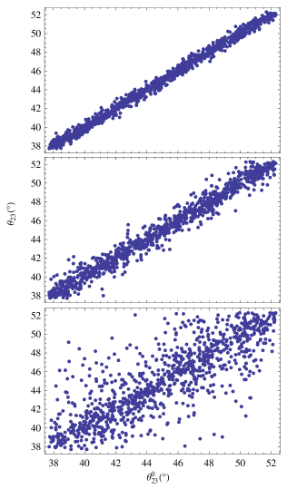
Figure 1: Correlation of $\theta_{23}$ (after perturbation) with $\theta_{23}^{0}$ (before perturbation). The lightest neutrino mass is (top to bottom) 0.001, 0.04 and 0.1 eV.

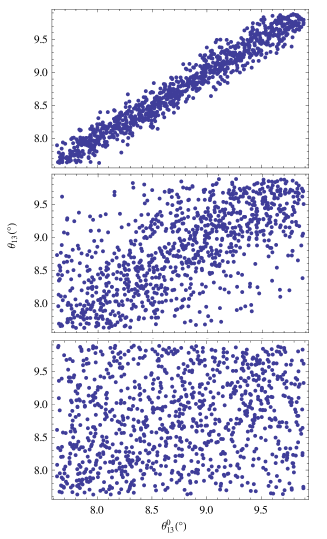
Figure 2: Correlation of $\theta_{13}$ (after perturbation) with $\theta_{13}^{0}$ (before perturbation). The lightest neutrino mass is (top to bottom) 0.001, 0.04 and 0.1 eV.

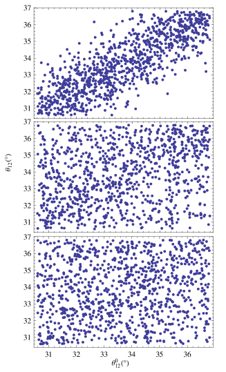
Figure 3: Correlation of $\theta_{12}$ (after perturbation) with $\theta_{12}^{0}$ (before perturbation). The lightest neutrino mass is (top to bottom) 0.001, 0.04 and 0.1 eV.

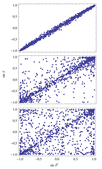
Figure 4: Correlation of $\sin\delta$ (after perturbation) with $\sin\delta^{0}$ (before perturbation). The lightest neutrino mass is (top to bottom) 0.001, 0.04 and 0.1 eV.

After these preliminaries, we evaluate now the percentages of the perturbed mass matrices that change the octant of $\theta_{23}$, the sign of $\sin\delta$ or the mass ordering (we do not consider Majorana phases, as their experimental determination is questionable). The results are shown in Figs. 5, 6 and 7. In the plots we indicate two interesting mass scales $\sqrt{\delta m^{2}}\simeq 0.008\textrm{ eV}$ and $\sqrt{\Delta m^{2}}\simeq 0.05\textrm{ eV}$, which will be discussed in detail later. We also plot the rather strong 95 % C.L. limit on neutrino masses (combining various cosmological data sets) as given by Planck Ade et al. (2014), $\sum m_{i}<0.23\textrm{ eV}$.

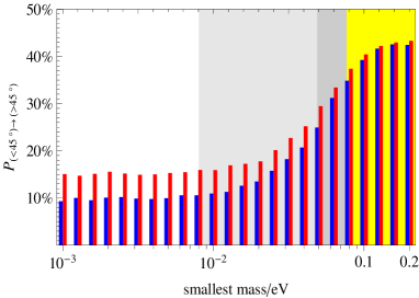
Figure 5: Percentage of perturbed mass matrices that give $\theta_{23}$ in the second octant when the unperturbed mass matrices give $\theta_{23}$ in the first octant (blue for normal mass ordering, red for inverted). The light-gray and gray regions start at $\sqrt{\delta m^{2}}\simeq 0.008\textrm{ eV}$ and $\sqrt{\Delta m^{2}}\simeq 0.05\textrm{ eV}$, respectively, while the yellow region represents the strongest cosmology constraint on neutrino masses Ade et al. (2014).

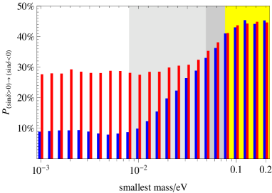
Figure 6: Percentage of perturbed mass matrices that give negative $\sin\delta$ when the unperturbed mass matrices give positive $\sin\delta$ (blue for normal mass ordering and red for inverted). For other details, see Fig. 5.

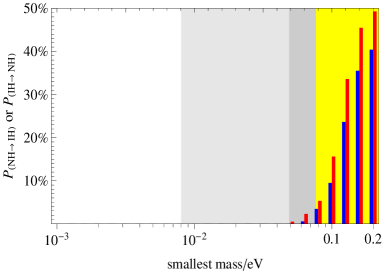
Figure 7: Percentage of perturbed mass matrices that give the inverted or normal mass ordering when the unperturbed mass matrices correspond to the normal (blue) or inverted (red) mass ordering, respectively. For other details, see Fig. 5.

II.3 Discussion

Very simple arguments are enough to understand the features of the results.

In Figs. 5, 6 7 we have indicated two relevant neutrino mass scales, $\sqrt{\delta m^{2}}\simeq 0.008\textrm{ eV}$ and $\sqrt{\Delta m^{2}}\simeq 0.05\textrm{ eV}$. Let us consider the normal mass ordering. Below the mass scale $\sqrt{\delta m^{2}}\simeq 0.008\textrm{ eV}$, all three mixing angles and the CP phase should be rather stable: neither $\delta m^{2}/(m_{1}^{2}+m_{2}^{2})$, associated to 12-mixing, nor $\Delta m^{2}/(m_{2}^{2}+m_{3}^{2})$, associated to 13- and 23-mixing, are small. However, when the smallest mass increases, first $\delta m^{2}/(m_{1}^{2}+m_{2}^{2})$ and then $\Delta m^{2}/(m_{2}^{2}+m_{3}^{2})$ decrease and become small. Consequently first $\theta_{12}$ and then $\theta_{13,23}$ will become unstable. Increasing the smallest mass further, corresponding to more and more quasi-degenerate masses, leads to all mixing angles becoming very unstable under perturbations.

From Fig. 3 we can see that for a smallest mass of $0.04\textrm{ eV}$, $\theta_{12}$ is unstable (since $\delta m^{2}/(m_{1}^{2}+m_{2}^{2})$ is small) as there is no significant correlation between $\theta_{12}$ and $\theta_{12}^{0}$. In contrast to $\theta_{12}$, $\theta_{13}$ and $\theta_{23}$ are more stable, as shown in Figs. 1 and 2. Increasing the smallest mass, $\theta_{23}$ and $\theta_{13}$ become unstable when $\Delta m^{2}/(m_{1}^{2}+m_{3}^{2})$ becomes small, which happens when the smallest mass goes beyond $\sqrt{\Delta m^{2}}\simeq 0.05\textrm{ eV}$.

More quantitative is Fig. 5. The probability of changing the octant is about 10 % for small masses and remains constant until the mass scale $\sqrt{\Delta m^{2}}\simeq 0.05\textrm{ eV}$ is reached. Approaching quasi-degenerate masses gives a probability of almost 50 % to change the octant, i.e. the octant is random and maximally unstable.

The predictions are more stable for the normal mass ordering than for the inverted one. This conclusion comes from the comparison of the relevant percentages in Figs. 5 and 6. Note that for a vanishing smallest mass we have $(m_{1}^{2},m_{2}^{2},m_{3}^{2})\approx(0,\delta m^{2},\Delta m^{2})$ for a normal ordering whereas for the inverted case we have $(m_{1}^{2},m_{2}^{2},m_{3}^{2})\approx(\Delta m^{2},\Delta m^{2}+\delta m^{2},0)$. Therefore, $\delta m^{2}/(m_{1}^{2}+m_{2}^{2})$ is small from the beginning and of order $\delta m^{2}/\Delta m^{2}\approx 0.03$. Indeed the probability to change the octant starts with about 15 % and increases when $\Delta m^{2}/(m_{1}^{2}+m_{3}^{2})$ becomes small for smallest masses of 0.05 eV and larger. Obviously for quasi-degenerate neutrino masses there will be no difference between the mass orderings.

Comparing Fig. 5 and 6, we can see that between $0.01\textrm{ eV}$ to $0.1\textrm{ eV}$, the probability of $\sin\delta$ changing its sign is larger than the probability of $\theta_{23}$ changing its octant. This is caused by the fact that phases of eigenvectors in a diagonalization procedure are always more sensitive to perturbation than their absolute values. One might also argue that $\delta$ is related to the Jarlskog invariant $J=$ Im$\left(U_{e1}\,U_{\mu 2}\,U_{e2}^{\ast}\,U_{\mu 1}^{\ast}\right)$ which is proportional to $\sin\delta\,\sin\theta_{12}\,\sin\theta_{13}\,\sin\theta_{23}$, which means that (for normal ordering) the probability of $\sin\delta$ changing its sign should be similar to the probability of $\theta_{23}$ changing the octant. That is indeed what Figs. 5 and 6 show. Note also that $J$ is proportional to the imaginary part of $h_{12}\,h_{23}\,h_{13}$, where $h=MM^{\dagger}$ Branco et al. (2003). For a negligible smallest mass $h$ has a dominating $23$-block in the normal mass ordering, whereas for the inverted ordering it has a democratic structure. Taking into account that predictions in the inverted ordering are in general less robust motivates to assume that the probability of $\sin\delta\rightarrow-\sin\delta$ is initially much larger than for the case of normal ordering. Indeed, see Fig. 6, one starts with almost 30 % for small masses. Again, for quasi-degenerate masses the sign is essentially random.

Interestingly, it is possible to change the mass ordering when perturbations are applied. This requires obviously quasi-degenerate neutrino masses, and Fig. 7 shows that for values around 0.1 eV the ordering can change, quickly reaching a probability of almost 50 %. For an inverted ordering the probability is larger and starts for smaller neutrino masses. This can be traced to the larger fine-tuning of neutrino masses in the inverted ordering: for a smallest neutrino mass of 0.2 eV, we have $(m_{1},m_{2},m_{3})=(0.2,0.200187,0.206004)$ eV in the normal ordering, but $(m_{3},m_{2},m_{1})=(0.2,0.205822,0.206004)$ eV in the inverted one (choosing the best-values of the mass-squared differences). Therefore, the heaviest and next-to-heaviest masses are much closer together in the inverted ordering. After adding a perturbation, switching from inverted to normal is thus more likely than the other way around.

III Perturbations on an $A_{4}$ model

In this section we will see how realistic our findings from the general case treated so far are. We apply corrections to a specific flavor symmetry model.

III.1 The model

We consider a model based on the discrete group $A_{4}$, as developed in Ma (2004); Altarelli and Feruglio (2005); Barry and Rodejohann (2010). In the unperturbed limit, the charged leptons are diagonal and the neutrino mass matrix is

$$M_{0}=\left(\begin{array}[]{ccc}\frac{2d}{3}&b-\frac{d}{3}&c-\frac{d}{3}\\ b-\frac{d}{3}&c+\frac{2d}{3}&-\frac{d}{3}\\ c-\frac{d}{3}&-\frac{d}{3}&b+\frac{2d}{3}\end{array}\right).$$ (3)

The mass-dimension parameters $b$ and $c$ are related to vacuum expectation values (VEVs) of $A_{4}$ singlets $\xi^{\prime\prime}$ and $\xi^{\prime}$, respectively. An $A_{4}$ triplet field $\varphi^{\prime}$ acquires VEVs in the $(1,1,1)$ direction and governs the parameter $d$:

$$\langle\xi^{\prime\prime}\rangle=u_{b}\,,\leavevmode\nobreak\ \thinspace\langle\xi^{\prime}\rangle=u_{c}\,,\leavevmode\nobreak\ \langle\varphi^{\prime}\rangle=v^{\prime}(1,1,1)\,,$$ (4)

with $b=u_{b}x_{b},c=u_{c}x_{c},d=v^{\prime}x_{d}$, and $x_{b,c,d}$ are dimensionless parameters.

Taking $b$, $c$ and $d$ as free parameters, the zeroth order mass matrix Eq. (3) can fit current neutrino data very well. To obtain the required parameters and to facilitate the perturbation, we minimize the following $\chi^{2}$-function:

$$\chi^{2}(b,c,d)\equiv\left(\frac{\theta_{23}-\theta_{23}^{0}}{\sigma_{23}}\right)^{2}+\left(\frac{\theta_{12}-\theta_{12}^{0}}{\sigma_{12}}\right)^{2}$$

$$+\left(\frac{\theta_{13}-\theta_{23}^{0}}{\sigma_{13}}\right)^{2}+\left(\frac{\delta m^{2}-\delta m_{0}^{2}}{\sigma_{\delta m^{2}}}\right)^{2}+\left(\frac{\Delta m^{2}-\Delta m_{0}^{2}}{\sigma_{\Delta m^{2}}}\right)^{2}$$

$$+\left(\frac{m-m_{\rm sm}}{\sigma_{m_{\rm sm}}\rightarrow 0}\right)^{2},$$ (5)

where the last term is added to fix the smallest mass, $m_{\rm sm}$, which is implemented by taking $\sigma_{m_{\rm sm}}\rightarrow 0$. In practice, we take $\sigma_{m_{\rm sm}}=m_{\rm sm}/1000$. The parameters $b$, $c$ and $d$ are, in general, complex numbers. We can remove an overall phase so only five degrees of freedom remain. The above mass matrix (3) is (partly) form-invariant, the eigenvector to the eigenvalue $b+c$ is always $(1,1,1)^{T}$, hence $|U_{e2}|^{2}=\frac{1}{3}$, independent of the magnitude of the mass matrix entries. Corrections will destroy this feature.

As usual in models of this kind, the parameters $b$, $c$ and $d$ have to be somewhat tuned to get the experimental values of $\delta m^{2}$ and $\Delta m^{2}$, which makes it technically difficult to find the minimum of the $\chi^{2}$-function. The $\chi^{2}$-fit gives the following conclusions:

1. The minimal value is non-zero, $\chi_{\rm min}^{2}=3.7$ which implies reasonable agreement with current data. The global minima are not unique but discrete, we find that there are four degenerate minima with $\chi_{\rm min}^{2}=3.7$;

2. The reason why we cannot have arbitrarily small $\chi^{2}$ is because of $|U_{e2}|^{2}=\frac{1}{3}$, which forces $\sin^{2}\theta_{12}$ to values larger than $\frac{1}{3}$ ($\sin^{2}\theta_{12}=0.341$, to be precise), while the $1\sigma$-range from global fits is below $\frac{1}{3}$. The other oscillation parameters can be reproduced to their best-fit values at the $\chi^{2}$-minimum, in particular we have Capozzi et al. (2014) $\sin^{2}\theta_{23}=0.437$. Due to the constraint $|U_{\alpha 2}|^{2}=\frac{1}{3}$, one has $\sqrt{2}\,|U_{e3}|\cos\delta\simeq 1/\tan 2\theta_{23}$, leading to $\delta=\pm 55.3^{\circ}$;

3. The degeneracy between the four minima corresponds to $(\delta,-\alpha_{1,2})\leftrightarrow(\delta,\alpha_{1,2})\leftrightarrow-(\delta,\alpha_{1,2})\leftrightarrow(-\delta,\alpha_{1,2})$. Here $\delta$ is the Dirac phase and $\alpha_{1,2}$ are Majorana phases. For $(\delta,\alpha_{1,2})\leftrightarrow-(\delta,\alpha_{1,2})$ the degeneracy is obvious since it means conjugating $M_{0}$. Henceforth, we name the four solutions $(+,+)$, $(+,-)$, $(-,+)$ and $(-,-)$ if the signs of $(\sin\delta,\sin\alpha_{1})$ are $(+,+)$, $(+,-)$, $(-,+)$ and $(-,-)$, respectively. The four discrete minima imply that for a fixed smallest mass, the model predicts definite CP phases, both Dirac and Majorana. Two of the four solutions have positive $\sin\delta$ and two negative;

4. We do not need to perturb these four zeroth order mass matrices separately, as the $(+,+)$ case is identical to the $(-,-)$ case, and the $(+,-)$ case identical to $(-,+)$;

5. For $m_{\rm sm}\mathrel{\hbox to0.0pt{\raise 2.20013pt\hbox{$<$}\hss}{\lower 2.20013pt\hbox{$\sim$}}}0.03$ eV (normal ordering) or $0.02$ eV (inverted ordering), there is no solution as $\chi_{\rm min}^{2}$ increases rapidly and soon gets out of the $5\sigma$ range. For values below, $\chi_{\rm min}^{2}$ is always $3.7$. The reason for this is the neutrino mass sum-rule $\tilde{m}_{3}-\tilde{m}_{1}=\tilde{m}_{2}$ (here $\tilde{m}_{i}$ are complex masses, thus including the Majorana phases), which implies Barry and Rodejohann (2011) the relations $m_{1}\mathrel{\hbox to0.0pt{\raise 2.20013pt\hbox{$>$}\hss}{\lower 2.20013pt\hbox{$\sim$}}}\sqrt{\Delta m^{2}}/\sqrt{3}$ and $m_{3}\mathrel{\hbox to0.0pt{\raise 2.20013pt\hbox{$>$}\hss}{\lower 2.20013pt\hbox{$\sim$}}}\sqrt{\Delta m^{2}}/2$, respectively.

III.2 Perturbation

For simplicity we study the following simple VEV misalignment:

$$\langle\xi^{\prime\prime}\rangle=u_{b}(1+\epsilon_{1})\,,\thinspace\langle\xi^{\prime}\rangle=u_{c}(1+\epsilon_{2})\,,$$ (6)

$$\langle\varphi^{\prime}\rangle=v^{\prime}(1+\epsilon_{3},1+\epsilon_{4},1+\epsilon_{5})\,.$$ (7)

As a result, the mass matrix is

$$M=\left(\begin{array}[]{ccc}\frac{2}{3}d\left(1+\epsilon_{3}\right)&b\left(1+\epsilon_{1}\right)-\frac{1}{3}d\left(1+\epsilon_{5}\right)&c\left(1+\epsilon_{2}\right)-\frac{1}{3}d\left(1+\epsilon_{4}\right)\\ b\left(1+\epsilon_{1}\right)-\frac{1}{3}d\left(1+\epsilon_{5}\right)&c\left(1+\epsilon_{2}\right)+\frac{2}{3}d\left(1+\epsilon_{4}\right)&-\frac{1}{3}d\left(1+\epsilon_{3}\right)\\ c\left(1+\epsilon_{2}\right)-\frac{1}{3}d\left(1+\epsilon_{4}\right)&-\frac{1}{3}d\left(1+\epsilon_{3}\right)&b\left(1+\epsilon_{1}\right)+\frac{2}{3}d\left(1+\epsilon_{5}\right)\end{array}\right).$$ (8)

Recall that the original $b,c,d$ are fixed by our initial $\chi^{2}$ minimization, so the various $\epsilon_{i}$ parameters are indeed required. Similar to our study of general perturbations, we randomly generate the $\epsilon$ and study the robustness of the mass matrix, i.e. the stability of the octant of $\theta_{23}$, the sign of $\sin\delta$ and the mass ordering. Figs. 8, 9 and 10 show the result. To illustrate our findings, we use $\sum|\epsilon_{i}|<0.04$ for Fig. 8 and Fig. 9, but $\sum|\epsilon_{i}|<0.2$ for Fig. 10; in addition we do not give results for all zeroth order solutions corresponding to the signs of the phases.

As one would expect from the general analysis in Section II, all percentages in the figures increase for increasing smallest mass. The normal mass ordering is somewhat more tuned than the inverted one, as the neutrino mass sum-rule $\tilde{m}_{3}-\tilde{m}_{1}=\tilde{m}_{2}$, which holds also after perturbation to good precision, requires more tuned Majorana phases in the normal ordering Barry and Rodejohann (2011). Therefore, the difference between normal and inverted ordering is not as large as in the general case, but the overall structure of the plots in Figs. 8, 9 and 10 is the same as in the general case.

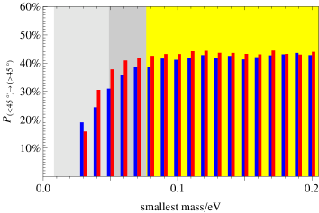
Figure 8: Change of octant: same as Fig. 5 for the $A_{4}$ model with VEV misalignment. Blue is the normal mass ordering, red inverted. The perturbation is made on the discrete solutions $(+,+)$ and $(-,-)$.

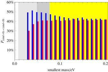
Figure 9: Change of the sign of $\sin\delta$: same as Fig. 6 for the $A_{4}$ model with VEV misalignment. Blue is the normal mass ordering, red inverted. The perturbation is made on the discrete solutions $(+,-)$ and $(-,+)$.

Figure 10: Change of mass ordering: same as Fig. 7 for the $A_{4}$ model with VEV misalignment. Blue is the normal mass ordering, red the inverted. The perturbation is made on the discrete solutions $(+,-)$ and $(-,+)$.

IV Conclusion

We have studied the robustness of neutrino mass matrix predictions in the general case and within a specific flavor symmetry model. We illustrate the need to include corrections to a mass matrix by showing that the octant of $\theta_{23}$, the sign of $\sin\delta$, or even the mass ordering can change when perturbations are added. Most of the results are intuitively clear: $\theta_{12}$ and $\delta$ are more unstable than $\theta_{13}$ and $\theta_{23}$, thus putting doubt on the discriminating power of the solar neutrino mixing angle and the CP phase when corrections are ignored. Predictions from an inverted mass ordering are more unstable than the normal one. The larger neutrino masses are, the more unstable are the predictions. Going beyond 0.1 eV can even change the mass ordering from normal to inverted, quickly reaching a probability of 50 %.

We have made here conservative assumptions about the perturbation parameters, namely multiplicative corrections. Additive corrections are expected to give qualitatively similar perturbations, but at least as sizable as the multiplicative ones under study here, as they influence small entries of the mass matrix more significantly. We have also not considered often and extensively studied charged lepton corrections, which are model-dependent and only influence the mixing matrix, independent of neutrino mass and mass ordering. At the current stage, we feel that our results already illustrate potential issues with the discriminative power of mass matrix predictions when perturbations are ignored, but at least illustrate quantitatively the potential impact they can have.