Inhomogeneous condensation in effective models for QCD using the finite-mode approach

Abstract

We use a numerical method, the finite-mode approach, to study inhomogeneous condensation in effective models for QCD in a general framework. Former limitations of considering a specific ansatz for the spatial dependence of the condensate are overcome. Different error sources are analyzed and strategies to minimize or eliminate them are outlined. The analytically known results for $1+1$ dimensional models (such as the Gross-Neveu model and extensions of it) are correctly reproduced using the finite-mode approach. Moreover, the NJL model in $3+1$ dimensions is investigated and its phase diagram is determined with particular focus on the inhomogeneous phase at high density.

I Introduction

Quantum Chromodynamics (QCD) cannot be solved analytically at low energies. However, several aspects of QCD can be understood by using effective models which exhibit the same symmetries as QCD, most notably chiral symmetry. Some models utilize exclusively hadronic degrees of freedom [such as chiral $\sigma$ models Meissner:1987ge ; Ko:1994en ; Urban:2001ru ; Gallas:2009qp ; Parganlija:2012fy ], while others feature constituent quarks [such as the Nambu–Jona-Lasinio (NJL) model Nambu:1961tp ; Nambu:1961fr ; Klevansky:1992qe ; Vogl:1991qt ; Hatsuda:1994pi ; Buballa:2003qv and the Gross-Neveu (GN) model Gross:1974jv ]. A model with both hadronic and quark degrees of freedom has also been discussed vanBeveren:2002mc ; Schaefer:2007pw .

All these effective descriptions of QCD include the spontaneous breaking of chiral symmetry, which implies the emergence of a chiral condensate at low temperatures and densities denoted as $\sigma$. This quantity is represented by a nonzero expectation value of a scalar-isoscalar mesonic field in hadronic chiral models or, equivalently, by the quark-antiquark expectation value $\langle\bar{\psi}\psi\rangle$ in quark-based models.

The chiral condensate is, in general, a function of space, $\sigma=\sigma(\vec{x})$. In principle, the determination of $\sigma(\vec{x})$ is straightforward: one has to find the field configuration which minimizes the effective action at a given temperature and density. In practice, this task is, however, very difficult. This is why $\sigma$ is often assumed to be spatially constant. This assumption is usually valid in the vacuum and at low densities, but not anymore at high densities. One of the simplest non-constant field configurations is the so-called chiral density wave (CDW) which, in chiral hadronic models, corresponds to a one-dimensional condensate of the form $\sigma(x_{3})=\phi\cos(px_{3})$ together with pion condensation, $\pi^{0}(x_{3})=\phi\sin(px_{3})$. Various studies have found that the CDW is favorable compared to a constant condensate at sufficiently high densities Baym:1973zk ; Sawyer:1973fv ; Campbell:1974qt ; Campbell:1974qu ; Dashen:1974ff ; Baym:1975tm ; Migdal:1978az ; Baym:1980jx ; Dickhoff:1981wk ; Kolehmainen:1982jn ; Baym:1982ca ; Akmal:1997ft . Interestingly, a CDW has recently also been obtained within the extended Linear Sigma Model Heinz:2013hza , which is a general chiral hadronic model with (axial-)vector degrees of freedom Gallas:2009qp ; Parganlija:2012fy . Moreover, inhomogeneous phases were also investigated in Refs. Broniowski:1989tw ; Sadzikowski:2000ap ; Casalbuoni:2005zp ; Nickel:2009wj ; Partyka:2010gk ; Broniowski:2011ef ; Carignano:2012sx ; Ma:2013vga ; Buballa:2014tba ; Kojo:2009ha ; Kojo:2011cn ; Harada:2015lma ; Carignano:2010ac ; Muller:2013tya in the framework of the NJL model as well as in the quark-meson model and the skyrmion model.

A general method to determine space-dependent condensates at non-zero temperature and density has not yet been established. There are a few exploratory studies of such methods in the context of the $1+1$ dimensional GN model, using either a lattice regularization deForcrand:2006zz of the effective action or an expansion in terms of plane waves or hat-like localized basis functions Wagner:2007he ; Wagner:2007av , but quite often one uses a specific Ansatz Nickel:2009wj ; Abuki:2011pf . More evolved models including three spatial dimensions and two-dimensional variations of the condensates and corresponding general methods, which are also based on expansions of fermionic fields and condensates in terms of plane waves, have been discussed theoretically in Refs. Nickel:2008ng ; Carignano:2012sx ; Cao:2015rea . In practice, however, due to limited computational resources, investigations have again been limited to specific Ansätze, where only a selected set of Fourier modes is considered, e.g. variations in only a single spatial dimension. In this respect models for which analytic inhomogeneous solutions are known are extremely interesting. This is the case for the $1+1$ dimensional GN model Thies:2003kk ; Basar:2009fg ; Ebert:2014woa ; Kojo:2014fxa ; Braun:2014fga , where a soliton-like solution for the spatial dependence of the condensate is found, which is mathematically represented by a Jacobi elliptic function Thies:2003kk ; Basar:2009fg . Further interesting $1+1$ dimensional models for which inhomogeneous phases have analytically been determined are extensions of the GN model: the chiral Gross-Neveu ($\chi$GN) model Salcedo:1990rw ; Dashen:1975xh , which has a continuous chiral symmetry, and the two-flavor NJL₂ model Ebert:2009mr . These $1+1$ dimensional models are relevant, because at high densities QCD effectively reduces from $3+1$ to $1+1$ dimensions McLerran:2007qj ; McLerran:2008ua ; Kojo:2009ha .

Thus, while the existence of inhomogeneous phases has been verified by several different approaches, it is highly desirable to develop a general and reliable numerical method to study inhomogeneous condensation, which does not require a specific ansatz for the spatial dependence of the condensate. This is the aim of the present work. We adapt and extend techniques introduced and explored in Refs. Wagner:2007he ; Wagner:2007av . We first test the validity and reliability of the resulting method, the finite-mode approach, by applying it to $1+1$ dimensional models, the GN, the $\chi$GN, and the NJL₂ model. We correctly reproduce both soliton-like and CDW modulations without supplying any specific ansatz.

Then we apply the finite-mode approach to study the phase structure of the $3+1$ dimensional NJL model. Recent findings Nickel:2009wj concerning one-dimensional modulations are confirmed. In addition, we determine the shape of the so-called inhomogeneous “continent” at high density Carignano:2011gr ; Carignano:2014jla : in agreement with these works, the phase boundary between chirally restored and inhomogeneous phase first increases with temperature. However, for larger chemical potential $\mu$ it decreases. Thus, the inhomogeneous phase exhibits a shape which is surprisingly similar to that of the crystal phase of the GN model.

The paper is organized as follows. In Sec. II quark-based effective models for QCD in $1+1$ and $3+1$ dimensions are introduced. In Sec. III, Sec. IV, Sec. V, and Sec. VI the phase diagrams of these models are investigated numerically using the finite-mode approach, with particular focus on inhomogeneous condensation. Finally, we present conclusions and an outlook in Sec. VII.

II Quark-based effective models

In this section we introduce the Lagrangians of the models that we use to investigate inhomogeneous condensation. We start with $1+1$ dimensional models and then turn to the $3+1$ dimensional NJL model.

II.1 $1+1$ dimensions: the GN model and its extensions

GN model

The GN model Gross:1974jv ; Wolff:1985av ; Thies:2003kk ; Basar:2009fg is a fermionic model that contains only a single quark flavor. In the large-$N$ limit (where $N$ is the number of colors) it exhibits QCD-like features such as asymptotic freedom, dynamical chiral symmetry breaking and its restoration, dimensional transmutation, and meson and baryon bound states tHooft:1973jz ; Witten:1979kh ; Lebed:1998st ; Schnetz:2005ih . The Lagrangian of the GN model in Euclidean space is

$$\mathcal{L}_{\text{GN}}=\sum_{j=1}^{N}\bar{\psi}_{j}\Big{(}\gamma_{\mu}\partial_{\mu}+m_{0}\Big{)}\psi_{j}-\frac{g^{2}}{2}\bigg{(}\sum_{j=1}^{N}\bar{\psi}_{j}\psi_{j}\bigg{)}^{2}\;,$$ (1)

with $\gamma_{0}=\sigma_{1}$ and $\gamma_{1}=\sigma_{3}$ implying $\gamma_{\mu}=\gamma_{\mu}^{\dagger}=\gamma_{\mu}^{\ast}$ and $\{\gamma_{\mu},\gamma_{\nu}\}=2\delta_{\mu\nu}$. Chiral symmetry is realized in a discrete way, $\psi_{j}\rightarrow\gamma_{5}\psi_{j}$. The term proportional to $m_{0}$ breaks chiral symmetry explicitly (it is analogous to a quark mass term). Therefore, in this work it is always set to zero, $m_{0}=0$ (similar choices are also implemented for the other models studied by us).

Spontaneous symmetry breaking is only realized in the limit $N\rightarrow\infty$ Gross:1974jv , since for any finite $N$ spontaneous symmetry breaking is excluded in $1+1$ dimensions Mermin:1966fe ; Coleman:1973ci . The chiral condensate arises upon condensation of the scalar-isoscalar field combination $\bar{\psi}_{j}\psi_{j}$, i.e., $\sigma=\langle\bar{\psi}_{j}\psi_{j}\rangle$ (where a sum over $j$ is implied).

In the limit $N\rightarrow\infty$ analytic solutions for thermodynamical quantities including inhomogeneous condensation have been found Schnetz:2005ih (see also the discussion in Sec. III).

$\chi$GN model

A straightforward extension of the GN model is obtained by adding a pseudoscalar term. The Lagrangian of the $\chi$GN model is

$$\mathcal{L}_{\chi\text{GN}}=\sum_{j=1}^{N}\bar{\psi}_{j}\gamma_{\mu}\partial_{\mu}\psi_{j}-\frac{g^{2}}{2}\bigg{[}\bigg{(}\sum_{j=1}^{N}\bar{\psi}_{j}\psi_{j}\bigg{)}^{2}+\bigg{(}\sum_{j=1}^{N}\bar{\psi}_{j}\imath\gamma_{5}\psi_{j}\bigg{)}^{2}\bigg{]}\;.$$ (2)

This model contains a scalar field combination $\bar{\psi}_{j}\psi_{j}$, which corresponds to a $\sigma$-like particle, and a pseudoscalar field combination $\bar{\psi}_{j}\imath\gamma_{5}\psi_{j}$, which corresponds to an $\eta$-like particle. It is invariant under continuous $U_{A}(1)$ chiral symmetry transformations, $\psi_{j}\rightarrow e^{\imath\theta\gamma_{5}}\psi_{j}$, and has certain similarities to one-flavor QCD (when the chiral anomaly is excluded).

The $\chi$GN model is particularly interesting, because both the scalar and the pseudoscalar field configurations condense, when the temperature exceeds a critical value. The ground state is then a CDW Schon:2000he ; Schon:2000qy .

NJL₂ model

A further extension of the GN model is obtained by considering, in addition to the scalar-isoscalar field combination, three pion-like field combinations. In this respect the model is similar to two-flavor QCD. The Lagrangian of this so-called NJL₂ model is

$$\mathcal{L}_{\text{NJL}_{2}}=\sum_{f=1}^{2}\sum_{j=1}^{N}\bar{\psi}_{j,f}\gamma_{\mu}\partial_{\mu}\psi_{j,f}-\frac{g^{2}}{2}\sum_{f=1}^{2}\bigg{[}\bigg{(}\sum_{j=1}^{N}\bar{\psi}_{j,f}\psi_{j,f}\bigg{)}^{2}+\bigg{(}\sum_{j=1}^{N}\bar{\psi}_{j,f}\vec{\tau}\imath\gamma_{5}\psi_{j,f}\bigg{)}^{2}\bigg{]}\;,$$ (3)

where $f=1,2$ is the flavor index. The model is invariant under chiral symmetry transformations $SU_{L}(2)\times SU_{R}(2)$,

$$\psi_{j,L}\rightarrow U_{L}\psi_{j,L}\quad,\quad\psi_{j,R}\rightarrow U_{R}\psi_{j,R}\;,$$ (4)

with

$$\psi_{j}=\left(\begin{array}[c]{c}\psi_{j,1}\\ \psi_{j,2}\end{array}\right)\quad,\quad\psi_{j,L}=P_{L}\psi_{j}\quad,\quad\psi_{j,R}=P_{R}\psi_{j}\;,$$ (5)

and $P_{L}$ and $P_{R}$ are projectors onto left- and right-handed components, respectively.

In contrast to the $\chi$GN model the ground state is not a CDW. Using the finite-mode approach we find that the phase diagram coincides with that of the GN model (cf. Sec. V).

II.2 $3+1$ dimensions: the NJL model

The NJL model in $3+1$ dimensions is one of the most famous effective chiral approaches to QCD. It has been extensively used in the vacuum and at non-zero temperature and density to study the spontaneous breaking of chiral symmetry and its restoration [cf. e.g. Refs. Bringoltz:2005rr ; Panero:2009tv ]. The Lagrangian (in the chiral limit for $N$ colors and two flavors) is Hatsuda:1994pi ; Klevansky:1992qe

$$\mathcal{L}_{\text{NJL}}=\sum_{f=1}^{2}\sum_{j=1}^{N}\bar{\psi}_{j,f}\gamma_{\mu}\partial_{\mu}\psi_{j,f}-\frac{3G}{N}\sum_{f=1}^{2}\bigg{[}\bigg{(}\sum_{j=1}^{N}\bar{\psi}_{j,f}\psi_{j,f}\bigg{)}^{2}+\bigg{(}\sum_{j=1}^{N}\bar{\psi}_{j,f}\vec{\tau}\imath\gamma_{5}\psi_{j,f}\bigg{)}^{2}\bigg{]}\;.$$ (6)

Chiral symmetry is realized in the same way as in the NJL₂ model [cf. Eqs. (4) and (5)].

In the vacuum, the quark field obtains an effective mass, if the coupling constant $G$ exceeds a critical value,

$$m_{0}^{\ast}=-\frac{6G}{N}\sum_{f=1}^{2}\sum_{j=1}^{N}\langle\bar{\psi}_{j,f}\psi_{j,f}\rangle>0\;.$$ (7)

This effective mass is proportional to the chiral condensate in the vacuum, i.e., $\sigma_{0}=-(N/6\sqrt{2}G)m_{0}^{\ast}$ Hatsuda:1994pi ; Klevansky:1992qe , where the chiral condensate is defined according to

$$\sigma=\frac{1}{\sqrt{2}}\sum_{f=1}^{2}\sum_{j=1}^{N}\langle\bar{\psi}_{j,f}\psi_{j,f}\rangle\;.$$ (8)

In other words, the field combination which gives rise to a non-zero condensate is again $\bar{\psi}_{j,f}\psi_{j,f}$. When restricting this condensate to be constant, chiral symmetry restoration at high densities occurs via a first-order phase transition Glendenning:2000wn ; Mishustin:1993ub ; Papazoglou:1997uw ; Papazoglou:1998vr ; Bonanno:2007kh . However, when allowing for an inhomogeneous condensate, the latter occurs at slightly smaller chemical potentials than the first-order phase transition. This is in agreement with the extended Linear Sigma Model results of Ref. Heinz:2013hza .

Contrary to the $1+1$ dimensional models of Sec. II.1, the NJL model is not renormalizable. The equation for $\sigma$ takes the form

$$\sigma_{0}=-2\sqrt{2}Nm_{0}^{\ast}\,I\quad\text{ with }\quad I=i\int\frac{d^{4}p}{(2\pi)^{4}}\frac{2}{p^{2}-m_{0}^{\ast 2}}=\int\frac{d^{3}p}{(2\pi)^{3}}\frac{1}{\sqrt{\vec{p}^{2}+m_{0}^{\ast 2}}}\;,$$ (9)

where the integral $I$ corresponds to a closed quark loop, i.e., to a tadpole diagram arising from the quartic NJL interaction of Eq. (6), which affects the quark propagator at the resummed one-loop level in the Hartree-Fock approximation [see Refs. Klevansky:1992qe ; Hatsuda:1994pi ; Vogl:1991qt for a detailed derivation].

The integral $I$ is, however, quadratically divergent. Indeed, the NJL model is properly defined only after a regularization scheme has been chosen and a corresponding high-energy scale enters as a new parameter. Strictly speaking, each choice of regularization corresponds to a different version of the NJL model. Once the regularization has been fixed, the quantity $m_{0}^{\ast}$ in Eq. (7) and, as a consequence, all the relevant thermodynamical quantities, are finite.

Especially in studies of the NJL model at nonzero density it is common to implement a three-dimensional cutoff [see e.g. Ref. Buballa:2003qv ] according to which

$$I\rightarrow I_{\Lambda}=\int_{0}^{\Lambda}\frac{d\left|\vec{p}\right|}{2\pi^{2}}\frac{\vec{p}^{2}}{\sqrt{\vec{p}^{2}+m_{0}^{\ast 2}}}\;.$$ (10)

Note that the use of a four-dimensional covariant cutoff is possible for studies of the vacuum Klevansky:1992qe ; Hatsuda:1994pi , but it is not easy to implement at nonzero temperatures and densities.

However, a three-dimensional cutoff strongly suppresses the appearance of inhomogeneous phases. Namely, in an inhomogeneous phase such as a CDW the quark propagator is not diagonal and the ingoing and outgoing momenta can differ by a full wavelength. This hardly takes place when the momentum $\left|\vec{p}\right|$ is limited by the cutoff $\Lambda$ Buballa:pri . Hence, in order to realize a CDW, other regularization approaches must be used, such as the Pauli-Villars scheme Carignano:2014jla or the proper-time regularization scheme Vogl:1991qt ; Hatsuda:1994pi ; Nakano:2004cd .

In this work we use the Pauli-Villars approach, which is a Lorentz (and gauge) invariant regularization procedure Klevansky:1992qe ; Itzykson:2006wn . It amounts to introduce $N_{\text{PV}}$ additional fictitious heavy fermions with mass $M_{k}$ in such a way that the tadpole integral of Eq. (9) is modified according to

$$I\rightarrow I_{\text{PV}}=\int\frac{\vec{p}^{2}d\left|\vec{p}\right|}{2\pi^{2}}\bigg{(}\frac{1}{\sqrt{\vec{p}^{2}+m_{0}^{\ast 2}}}+\sum_{k=1}^{N_{PV}}\frac{C_{k}}{\sqrt{\vec{p}^{2}+M_{k}^{2}}}\bigg{)}\;,$$ (11)

with the masses given by

$$M_{k}^{2}=m_{0}^{\ast 2}+\alpha_{k}\Lambda_{\text{PV}}^{2}\;,$$ (12)

where $\Lambda_{\text{PV}}$ is the so-called Pauli-Villars high-energy scale. The constants $C_{k}$ and $\alpha_{k}$ are real dimensionless numbers, which are chosen in such a way that $I_{PV}$ is finite. Let us show this explicitly for the case $N_{\text{PV}}=2$. For large values of $\vec{p}^{2}$ the quantity in parentheses in Eq. (11) can be approximated by a Taylor expansion,

$$(\ldots)=\frac{1}{\left|\vec{p}\right|}\bigg{[}1+C_{1}+C_{2}-\frac{1}{2}\frac{m_{0}^{\ast 2}(1+C_{1}+C_{2})+\Lambda^{2}_{\mathrm{PV}}(\alpha_{1}C_{1}+\alpha_{2}C_{2})}{\left|\vec{p}\right|^{2}}+\mathcal{O}(\left|\vec{p}\right|^{-4})\bigg{]}\;.$$ (13)

Then, by requiring

$$1+C_{1}+C_{2}=0\quad\text{ and }\quad\alpha_{1}C_{1}+\alpha_{2}C_{2}=0$$ (14)

the integrand of Eq. (11) falls off as $\left|\vec{p}\right|^{-3}$ and is, therefore, convergent (although it explicitly depends on the scale $\Lambda_{\text{PV}}$). Once $I_{\text{PV}}$ is finite, the quark condensate, the quark mass, as well as all other relevant quantities are also finite. The conditions in Eq. (14) are met for $\alpha_{1}=2$ and $\alpha_{2}=1$ with $C_{1}=1$ and $C_{2}=-2$.

The procedure can be easily generalized to an arbitrary number of heavy fermions $N_{\mathrm{PV}}$,

$$1+\sum_{k=1}^{N_{\mathrm{PV}}}C_{k}=0\quad,\quad\sum_{k=1}^{N_{\mathrm{PV}}}\alpha_{k}C_{k}=0\;.$$ (15)

For the case $N_{\mathrm{PV}}=3$ the previous equations are fulfilled by $\alpha_{1}=1$, $\alpha_{2}=2$, $\alpha_{3}=3$ and $C_{1}=-3$, $C_{2}=3$ , $C_{3}=-1$. In Sec. VI we will compute the phase diagram of the NJL model with inhomogeneous condensation using the Pauli-Villars regularization with two and three heavy fermions.

III Finite-mode regularization of the $1+1$ dimensional GN model

In the following we discuss the finite-mode approach in detail, in particular its technical aspects, in the context of the $1+1$ dimensional GN model in the large-$N$ limit [cf. also Refs. Andrianov:1982sn ; Andrianov:1983fg ; Andrianov:1983qj ; Wagner:2007he ; Wagner:2007av ]. We reproduce the analytically known phase diagram, which exhibits an inhomogeneous crystal phase.

III.1 Partition function and Euclidean action

The partition function of the 1+1 dimensional GN model (1) in Euclidean spacetime is

$$Z=\int\bigg{(}\prod_{j=1}^{N}D\bar{\psi}_{j}D\psi_{j}\bigg{)}e^{-S_{E}[\psi_{j},\bar{\psi}_{j}]}\;,$$ (16)

with the action

$$S_{E}[\bar{\psi}_{j},\psi_{i}]=\int d^{2}x\,\bigg{[}\sum_{j=1}^{N}\bar{\psi}_{j}\Big{(}\gamma_{\mu}\partial_{\mu}+\gamma_{0}\mu\Big{)}\psi_{j}-\frac{g^{2}}{2}\bigg{(}\sum_{j=1}^{N}\bar{\psi}_{j}\psi_{j}\bigg{)}^{2}\bigg{]}\;,$$ (17)

where $\mu$ is the chemical potential. One can get rid of the four-fermion term by introducing a real scalar field $\sigma$,

$$Z=\int D\sigma\,\bigg{(}\prod_{j=1}^{N}D\bar{\psi}_{j}D\psi_{j}\bigg{)}\exp\bigg{[}-\int d^{2}x\,\bigg{(}\frac{1}{2g^{2}}\sigma^{2}+\sum_{j=1}^{N}\bar{\psi}_{j}Q\psi_{j}\bigg{)}\bigg{]}\;,$$ (18)

with the Dirac operator

$$Q=\gamma_{\mu}\partial_{\mu}+\gamma_{0}\mu+\sigma\;.$$ (19)

Performing the integration over the fermionic fields results in

$$Z=\int D\sigma\,(\det Q)^{N}\exp\bigg{(}-\frac{1}{2g^{2}}\sigma^{2}\bigg{)}\;.$$ (20)

Since $\det Q$ is real fn , $(\det Q)^{2}=\det(Q^{\dagger}Q)\geq 0$. Consequently, for even $N$

$$Z=\int D\sigma\,e^{-S_{E,\text{eff}}[\sigma]}\quad,\quad S_{E,\text{eff}}[\sigma]=N\int d^{2}x\,\bigg{\{}\frac{1}{2\lambda}\sigma^{2}-\frac{1}{2}\ln[\det(Q^{\dagger}Q)]\bigg{\}}\;,$$ (21)

where $\lambda=Ng^{2}$. Due to numerical reasons discussed in detail in Ref. Wagner:2007he , when using the finite-mode approach it is highly advantageous to regularize the effective action expressed in terms of $\det(Q^{\dagger}Q)$ instead of the mathematically equivalent expression containing $\det Q$.

III.2 Finite-mode regularization, homogeneous condensate $\sigma=\text{constant}$

For numerical calculations it is convenient to work exclusively with dimensionless quantities. Therefore, we express all dimensionful quantities in units of $\sigma_{0}$ which is the non-vanishing value of the constant condensate $\sigma$ at temperature $T=0$ and chemical potential $\mu=0$. The resulting dimensionless quantities are denoted by a hat $\hat{\phantom{x}}$, e.g. $\hat{x}_{\mu}=x_{\mu}\sigma_{0}$, $\hat{T}=T/\sigma_{0}$, $\hat{\mu}=\mu/\sigma_{0}$, $\hat{\sigma}=\sigma/\sigma_{0}$, etc.

We consider a finite spacetime volume with temporal extension $\hat{L}_{0}=L_{0}\sigma_{0}$ (corresponding to the inverse temperature $1/\hat{T}=\hat{L}_{0}$) and spatial extension $\hat{L}_{1}=L_{1}\sigma_{0}$. The fermionic fields are expressed as superpositions of plane waves with periodic boundary conditions in spatial direction and antiperiodic boundary conditions in temporal direction,

$$\hat{\psi}_{j}(\hat{x}_{0},\hat{x}_{1}) =\frac{\psi_{j}(x_{0},x_{1})}{\sqrt{\sigma_{0}}}=\sum_{n_{0},n_{1}}\eta_{j,n_{0},n_{1}}\frac{e^{-\imath(\hat{k}_{0}\hat{x}_{0}+\hat{k}_{1}\hat{x}_{1})}}{\sqrt{\hat{L}_{0}\hat{L}_{1}}}\;,$$ (22)

$$\hat{\bar{\psi}}_{j}(\hat{x}_{0},\hat{x}_{1}) =\frac{\bar{\psi}_{j}(x_{0},x_{1})}{\sqrt{\sigma_{0}}}=\sum_{n_{0},n_{1}}\bar{\eta}_{j,n_{0},n_{1}}\frac{e^{+\imath(\hat{k}_{0}\hat{x}_{0}+\hat{k}_{1}\hat{x}_{1})}}{\sqrt{\hat{L}_{0}\hat{L}_{1}}}\;,$$ (23)

with discrete momenta

$$\hat{k}_{0}=\frac{2\pi}{\hat{L}_{0}}\left(n_{0}-\frac{1}{2}\right)\quad,\quad\hat{k}_{1}=\frac{2\pi}{\hat{L}_{1}}n_{1}\quad,\quad n_{0},n_{1}\in\mathbb{N}\;,$$

where $\eta_{j,n_{0},n_{1}}$ and $\bar{\eta}_{j,n_{0},n_{1}}$ are dimensionless Grassmann variables.

For a homogeneous condensate $\sigma=\text{constant}$, $\ln[\det(\hat{Q}^{\dagger}\hat{Q})]$ can be expressed as a product over the modes $(\hat{k}_{0},\hat{k}_{1})$,

$$\ln[\det(\hat{Q}^{\dagger}\hat{Q})]=\ln\bigg{\{}\prod_{\hat{k}_{0},\hat{k}_{1}}\det\Big{[}\Big{(}+\imath\gamma_{\mu}\hat{k}_{\mu}-\gamma_{0}\hat{\mu}+\hat{\sigma}\Big{)}\Big{(}-\imath\gamma_{\mu}\hat{k}_{\mu}+\gamma_{0}\hat{\mu}+\hat{\sigma}\Big{)}\Big{]}\bigg{\}}$$

$$\hskip 14.22636pt=\ln\bigg{\{}\prod_{\hat{k}_{0},\hat{k}_{1}}\Big{[}(\hat{k}_{0}^{2}+\hat{k}_{1}^{2}+\hat{\sigma}^{2}-\hat{\mu}^{2})^{2}+(2\hat{\mu}\hat{k}_{0})^{2}\Big{]}\bigg{\}}\;.$$ (24)

Considering only a finite number of modes $n_{0}=-N_{0}+1,-N_{0}+2,\ldots,N_{0}-1,N_{0}$ and $n_{1}=-N_{1},-N_{1}+1,\ldots,N_{1}-1,N_{1}$, i.e., introducing momentum cutoffs

$$\hat{k}_{0}^{\text{cut}}=\frac{2\pi}{\hat{L}_{0}}N_{0}\quad,\quad\hat{k}_{1}^{\text{cut}}=\frac{2\pi}{\hat{L}_{1}}\left(N_{1}+\frac{1}{2}\right)\;,$$ (25)

(chosen to be $\pi/\hat{L}_{0,1}$ larger than the largest momenta considered) yields the finite-mode regularized effective action,

$$\frac{S_{E,\text{eff}}(\hat{\sigma})}{N}=\frac{\hat{L}_{0}\hat{L}_{1}\hat{\sigma}^{2}}{2\lambda}$$

$$\hskip 28.45274pt-\frac{1}{2}\sum_{n_{0}=-N_{0}+1}^{N_{0}}\sum_{n_{1}=-N_{1}}^{N_{1}}\ln\bigg{(}\bigg{\{}\bigg{[}\frac{2\pi}{\hat{L}_{0}}\left(n_{0}-\frac{1}{2}\right)\bigg{]}^{2}+\bigg{(}\frac{2\pi}{\hat{L}_{1}}n_{1}\bigg{)}^{2}+\hat{\sigma}^{2}-\hat{\mu}^{2}\bigg{\}}^{2}+\bigg{[}2\hat{\mu}\frac{2\pi}{\hat{L}_{0}}\left(n_{0}-\frac{1}{2}\right)\bigg{]}^{2}\bigg{)}$$

$$\hskip 14.22636pt=\frac{2\pi^{2}N_{0}(N_{1}+1/2)\hat{\sigma}^{2}}{\lambda\hat{k}_{0}^{\text{cut}}\hat{k}_{1}^{\text{cut}}}$$

$$\hskip 28.45274pt-\sum_{n_{0}=1}^{N_{0}}\sum_{n_{1}=-N_{1}}^{N_{1}}\ln\bigg{\{}\bigg{[}\bigg{(}\hat{k}_{0}^{\text{cut}}\frac{n_{0}-1/2}{N_{0}}\bigg{)}^{2}+\bigg{(}\hat{k}_{1}^{\text{cut}}\frac{n_{1}}{N_{1}+1/2}\bigg{)}^{2}+\hat{\sigma}^{2}-\hat{\mu}^{2}\bigg{]}^{2}+\bigg{(}2\hat{\mu}\hat{k}_{0}^{\text{cut}}\frac{n_{0}-1/2}{N_{0}}\bigg{)}^{2}\bigg{\}}\;,$$ (26)

which is suitable for numerical evaluation. Minimizing this effective action with respect to $\hat{\sigma}$ for various $\hat{\mu}$ and $\hat{T}$ yields $\hat{\sigma}(\hat{\mu},\hat{T})$, i.e., the “homogeneous phase diagram of the GN model” Wolff:1985av .

Infinite-volume continuum results are obtained in the limit $\hat{L}_{1}\rightarrow\infty$, $\hat{k}_{0}^{\text{cut}}\rightarrow\infty$, and $\hat{k}_{1}^{\text{cut}}\rightarrow\infty$, which implies an infinite number of modes. Numerically one is, of course, restricted to a finite number of modes. In the following we discuss how to determine the parameters $\lambda$, $N_{0}$, $N_{1}$, $\hat{k}_{0}^{\text{cut}}$, and $\hat{k}_{1}^{\text{cut}}$ [$\hat{L}_{0}$ and $\hat{L}_{1}$ are then given by Eq. (25)] in an optimal way, i.e., how to obtain numerical results with a finite and rather limited number of modes, which are nevertheless very close to infinite-volume continuum results.

III.3 Choosing and determining suitable parameters $\lambda$, $N_{0}$, $N_{1}$, $\hat{k}_{0}^{\text{cut}}$, and $\hat{k}_{1}^{\text{cut}}$

The condensate $\hat{\sigma}$ minimizes the effective action (III.2). For $\mu=0$ it is the solution of

$$0=\frac{d}{d\hat{\sigma}}\frac{S_{E,\text{eff}}(\hat{\sigma})}{N}=2\hat{\sigma}\bigg{\{}\frac{2\pi^{2}N_{0}(N_{1}+1/2)}{\lambda\hat{k}_{0}^{\text{cut}}\hat{k}_{1}^{\text{cut}}}-2\sum_{n_{0}=1}^{N_{0}}\sum_{n_{1}=-N_{1}}^{N_{1}}\bigg{[}\bigg{(}\hat{k}_{0}^{\text{cut}}\frac{n_{0}-1/2}{N_{0}}\bigg{)}^{2}+\bigg{(}\hat{k}_{1}^{\text{cut}}\frac{n_{1}}{N_{1}+1/2}\bigg{)}^{2}+\hat{\sigma}^{2}\bigg{]}^{-1}\bigg{\}}\;.$$ (27)

An obvious solution is $\hat{\sigma}=0$. It corresponds to a minimum for $T>T_{c}$ and to a maximum for $T\leq T_{c}$. For the latter case there are two additional solutions (corresponding to minima), which can be obtained from

$$0=\frac{2\pi^{2}N_{0}(N_{1}+1/2)}{\lambda\hat{k}_{0}^{\text{cut}}\hat{k}_{1}^{\text{cut}}}-2\sum_{n_{0}=1}^{N_{0}}\sum_{n_{1}=-N_{1}}^{N_{1}}\bigg{[}\bigg{(}\hat{k}_{0}^{\text{cut}}\frac{n_{0}-1/2}{N_{0}}\bigg{)}^{2}+\bigg{(}\hat{k}_{1}^{\text{cut}}\frac{n_{1}}{N_{1}+1/2}\bigg{)}^{2}+\hat{\sigma}^{2}\bigg{]}^{-1}\;.$$ (28)

To appropriately determine the parameters $\lambda$, $N_{0}$, $N_{1}$, $\hat{k}_{0}^{\text{cut}}$, and $\hat{k}_{1}^{\text{cut}}$, we consider and relate computations at $\mu=0$ and a low temperature $T\approx 0$, where $\sigma(T)\approx\sigma_{0}$, and at $\mu=0$ and the critical temperature $T=T_{c}$, where $\sigma$ just vanishes, i.e., $\sigma(T-\epsilon)>0$ and $\sigma(T)=0$. The parameters $\lambda$, $N_{1}$, $\hat{k}_{0}^{\text{cut}}$, and $\hat{k}_{1}^{\text{cut}}$ are the same for both simulations, while $N_{0}=N_{00}$ for $T\approx 0$ and $N_{0}=N_{0c}\ll N_{00}$ for $T=T_{c}$.

The parameters $N_{0c}$, $N_{00}$, $N_{1}$, and $\hat{k}_{1}^{\text{cut}}$ can be chosen independently. The maximum number of modes $\propto N_{00}N_{1}$ is, of course, limited by the available computer resources. Strategies for choosing these four parameters in an optimal way, i.e., where systematic errors due to the finite spatial extension and the finite number of modes are minimized, are discussed in Secs. III.3.1, III.3.2, and III.3.3 below.

In contrast to that, $\hat{k}_{0}^{\text{cut}}$ and $\lambda$ cannot be chosen independently: $\hat{k}_{0}^{\text{cut}}=2\pi N_{0c}\hat{T}_{c}$ [which follows from Eq. (25)], i.e., $\hat{k}_{0}^{\text{cut}}$ is related to $N_{0c}$. Since $\hat{T}_{c}$ is a priori unknown, setting $\hat{k}_{0}^{\text{cut}}$ to an appropriate value is a non-trivial task. Similarly, $\lambda$ depends on $N_{0c}$, $N_{1}$, $\hat{k}_{0}^{\text{cut}}$, and $\hat{k}_{1}^{\text{cut}}$ via Eq. (28) at $T=T_{c}$, where $\hat{\sigma}=0$,

$$\frac{\pi^{2}(N_{1}+1/2)}{\lambda\hat{k}_{0}^{\text{cut}}\hat{k}_{1}^{\text{cut}}}=\frac{1}{N_{0c}}\sum_{n_{0}=1}^{N_{0c}}\sum_{n_{1}=-N_{1}}^{N_{1}}\bigg{[}\bigg{(}\hat{k}_{0}^{\text{cut}}\frac{n_{0}-1/2}{N_{0c}}\bigg{)}^{2}+\bigg{(}\hat{k}_{1}^{\text{cut}}\frac{n_{1}}{N_{1}+1/2}\bigg{)}^{2}\bigg{]}^{-1}\;.$$ (29)

To determine $\hat{k}_{0}^{\text{cut}}$ (without knowing $\hat{T}_{c}$), we consider Eq. (28) also for $T\approx 0$, where $\hat{\sigma}\approx 1$, i.e.,

$$\frac{\pi^{2}(N_{1}+1/2)}{\lambda\hat{k}_{0}^{\text{cut}}\hat{k}_{1}^{\text{cut}}}=\frac{1}{N_{00}}\sum_{n_{0}=1}^{N_{00}}\sum_{n_{1}=-N_{1}}^{N_{1}}\bigg{[}\bigg{(}\hat{k}_{0}^{\text{cut}}\frac{n_{0}-1/2}{N_{00}}\bigg{)}^{2}+\bigg{(}\hat{k}_{1}^{\text{cut}}\frac{n_{1}}{N_{1}+1/2}\bigg{)}^{2}+1\bigg{]}^{-1}\;.$$ (30)

Since the left-hand sides of Eqs. (29) and (30) are identical, we can equate their right-hand sides and eliminate $\lambda$,

$$\sum_{n_{1}=-N_{1}}^{N_{1}}\bigg{\{}\frac{1}{N_{0c}}\sum_{n_{0}=1}^{N_{0c}}\bigg{[}\bigg{(}\hat{k}_{0}^{\text{cut}}\frac{n_{0}-1/2}{N_{0c}}\bigg{)}^{2}+\bigg{(}\hat{k}_{1}^{\text{cut}}\frac{n_{1}}{N_{1}+1/2}\bigg{)}^{2}\bigg{]}^{-1}$$

$$\hskip 28.45274pt-\frac{1}{N_{00}}\sum_{n_{0}=1}^{N_{00}}\bigg{[}\bigg{(}\hat{k}_{0}^{\text{cut}}\frac{n_{0}-1/2}{N_{00}}\bigg{)}^{2}+\bigg{(}\hat{k}_{1}^{\text{cut}}\frac{n_{1}}{N_{1}+1/2}\bigg{)}^{2}+1\bigg{]}^{-1}\bigg{\}}=0\;.$$ (31)

For given $N_{0c}$, $N_{00}$, $N_{1}$, and $\hat{k}_{1}^{\text{cut}}$ one has to solve this equation to obtain $\hat{k}_{0}^{\text{cut}}$. Then, $\lambda$ can be calculated using either Eq. (29) or (30).

III.3.1 Optimizing $N_{0c}$

The numerically obtained critical temperature $\hat{T}_{c}=\hat{k}_{0}^{\text{cut}}/2\pi N_{0c}$ should be insensitive with respect to variations of $N_{0c}$, when keeping the other parameters fixed, in particular $N_{00}$. The corresponding optimal $N_{0c}^{\text{opt}}$ is, therefore, defined as the value of $N_{0c}$ which minimizes

$$\bigg{|}\frac{\partial}{\partial N_{0c}}\hat{T}_{c}\bigg{|}$$ (32)

(since $N_{0c}\in\mathbb{N}$, the derivative $\partial/\partial N_{0c}$ has to be understood as a finite difference).

To study this optimization of $N_{0c}$ independently of any error due to the finite spatial momentum cutoff $\hat{k}_{1}^{\text{cut}}$ and the finite spatial extension $\hat{L}_{1}=2\pi(N_{1}+1/2)/\hat{k}_{1}^{\text{cut}}$, we consider for a moment the limit $\hat{k}_{1}^{\text{cut}}\rightarrow\infty$ and $\hat{L}_{1}\rightarrow\infty$ (implying $N_{1}\rightarrow\infty$). In this limit

$$\hat{k}_{1}^{\text{cut}}\frac{n_{1}}{N_{1}+1/2}\rightarrow\hat{k}_{1}\quad,\quad\frac{\hat{k}_{1}^{\text{cut}}}{N_{1}+1/2}\rightarrow d\hat{k}_{1}\quad,\quad\frac{N_{1}}{\hat{k}_{1}^{\text{cut}}}\sum_{n_{1}=-N_{1}}^{N_{1}}\frac{\hat{k}_{1}^{\text{cut}}}{N_{1}+1/2}\rightarrow\frac{N_{1}+1/2}{\hat{k}_{1}^{\text{cut}}}\int d\hat{k}_{1}\;.$$ (33)

Inserting these relations into Eq. (III.3) and solving the integral results in

$$\frac{1}{N_{0c}}\sum_{n_{0}=1}^{N_{0c}}\bigg{(}\hat{k}_{0}^{\text{cut}}\frac{n_{0}-1/2}{N_{0c}}\bigg{)}^{-1}-\frac{1}{N_{00}}\sum_{n_{0}=1}^{N_{00}}\bigg{[}\bigg{(}\hat{k}_{0}^{\text{cut}}\frac{n_{0}-1/2}{N_{00}}\bigg{)}^{2}+1\bigg{]}^{-1/2}=0\;.$$ (34)

As previously Eq. (III.3) this equation has to be solved to obtain $\hat{k}_{0}^{\text{cut}}$, which now only depends on $N_{0c}$ and $N_{00}$.

In FIG. 1 we study the corresponding $\hat{T}_{c}=\hat{k}_{0}^{\text{cut}}/2\pi N_{0c}$ as a function of $N_{0c}$ (left panel) and $N_{0c}/N_{00}$ (right panel) for $N_{00}\in\{64,128,256\}$:

• For sufficiently large $N_{00}$ and a suitably chosen $N_{0c}$ the resulting $\hat{T}_{c}$ should be close to the analytically known infinite-volume continuum result $\hat{T}_{c}=e^{C}/\pi\approx 0.566$ (where $C$ denotes Euler’s constant) Wolff:1985av . One can clearly see that there are plateau-like regions, where this is the case.

• For a small number of temporal modes $N_{0c}$ there are strong deviations, because the temporal momentum cutoff is rather small, $\hat{k}_{0}^{\text{cut}}=2\pi N_{0c}\hat{T}_{c}$ (for small $N_{0c}$, curves obtained with different $N_{00}$ fall on top of each other when plotted versus $N_{0c}\propto\hat{k}_{0}^{\text{cut}}$).

• For $N_{0c}/N_{00}\raisebox{-2.15277pt}{$\,\stackrel{{\scriptstyle>}}{{\scriptstyle\sim}}\,$}0.2$ there are also strong deviations, because the temperature corresponding to $N_{00}$ temporal modes, $\hat{T}_{0}=\hat{T}_{c}N_{0c}/N_{00}$, is a poor approximation of zero temperature (for $N_{0c}/N_{00}\raisebox{-2.15277pt}{$\,\stackrel{{\scriptstyle>}}{{\scriptstyle\sim}}\,$}0.2$, curves obtained with different $N_{00}$ fall on top of each other when plotted versus $N_{0c}/N_{00}=\hat{T}_{0}/\hat{T}_{c}$).

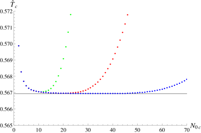
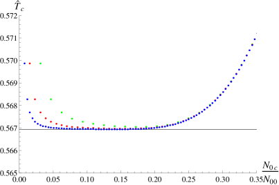
Figure 1: $\hat{T}_{c}$ as a function of $N_{0c}$ (left panel) and $N_{0c}/N_{00}$ (right panel) for $N_{00}=64$ (green dots), $N_{00}=128$ (red dots), and $N_{00}=256$ (blue dots) obtained from Eq. (34) (the black lines indicate the infinite-volume continuum result $\hat{T}_{c}=e^{C}/\pi$).

In other words, to obtain accurate results, $1\ll N_{0c}\ll N_{00}$ has to be fulfilled, which is only possible, if a sufficiently large number of temporal modes $N_{00}$ are used. According to the definition (32) the optimal $N_{0c}$ for given $N_{00}$ is the minimum of the corresponding curves in FIG. 1.

In TABLE 1 one can see the accuracy $1-\hat{T}_{c}/(e^{C}/\pi)$ of the numerically obtained $\hat{T}_{c}$, for various values of $N_{00}$. Note that even with a comparatively small number of $N_{00}=32$ temporal modes, the error is less than $0.1\%$. Also listed in TABLE 1 are $N_{0c}^{\text{opt}}$, the corresponding temporal momentum cutoff $\hat{k}_{0}^{\text{cut,opt}}=2\pi N_{0c}^{\text{opt}}\hat{T}_{c}$, and the corresponding temporal extension $\hat{L}_{00}^{\text{opt}}=N_{00}/\hat{T}_{c}N_{0c}^{\text{opt}}$ approximating $T=0$. When increasing $N_{00}$, there is a similar increase in the temporal momentum cutoff $\hat{k}_{0}^{\text{cut,opt}}$, but only a slight increase in the temporal extension $\hat{L}_{00}^{\text{opt}}$. This is typical for lattice calculations, where cutoff effects are only polynomially suppressed, while finite-volume effects are exponentially suppressed.

$N_{00}$	$1-\hat{T}_{c}/(e^{C}/\pi)$	$N_{0c}^{\text{opt}}$	$\hat{k}_{0}^{\text{cut,opt}}$	$\hat{L}_{00}^{\text{opt}}$
$32$	$-6.320\cdot 10^{-4}$	$6$	$2.139\cdot 10^{1}$	$9.401$
$64$	$-1.981\cdot 10^{-4}$	$11$	$3.919\cdot 10^{1}$	$10.26$
$128$	$-6.158\cdot 10^{-5}$	$20$	$7.125\cdot 10^{1}$	$11.29$
$256$	$-1.881\cdot 10^{-5}$	$36$	$1.282\cdot 10^{2}$	$12.54$
$512$	$-5.650\cdot 10^{-6}$	$66$	$2.350\cdot 10^{2}$	$13.68$
$1024$	$-1.672\cdot 10^{-6}$	$120$	$4.275\cdot 10^{2}$	$15.05$
$2048$	$-4.886\cdot 10^{-7}$	$222$	$7.908\cdot 10^{2}$	$16.27$
$4096$	$-1.413\cdot 10^{-7}$	$412$	$1.468\cdot 10^{3}$	$17.53$

Table 1: Accuracy of the numerically obtained $\hat{T}_{c}$ for various values of $N_{00}$.

III.3.2 Optimizing $\hat{k}_{1}^{\text{cut}}$

In the following we investigate the error associated with a finite spatial momentum cutoff $\hat{k}_{1}^{\text{cut}}$, i.e., instead of Eq. (34) we return to Eq. (III.3) and solve this equation to obtain $\hat{k}_{0}^{\text{cut}}$ for given $N_{0c}$, $N_{00}$, $N_{1}$, and $\hat{k}_{1}^{\text{cut}}$. Similarly to Sec. III.3.1 we define the optimal $\hat{k}_{1}^{\text{cut},\text{opt}}$ as the value of $\hat{k}_{1}^{\text{cut}}$ which minimizes

$$\bigg{|}\frac{\partial}{\partial\hat{k}_{1}^{\text{cut}}}\hat{T}_{c}\bigg{|}$$ (35)

for given $N_{0c}$, $N_{00}$, and $N_{1}$.

We choose $N_{00}=256$, the corresponding optimal $N_{0c}=36$ (cf. TABLE 1) and various numbers of spatial modes $N_{1}$. In FIG. 2 we study $\hat{T}_{c}=\hat{k}_{0}^{\text{cut}}/2\pi N_{0c}$ as a function of $\hat{k}_{1}^{\text{cut}}$ (left panel) and $\hat{k}_{1}^{\text{cut}}/(N_{1}+1/2)$ (right panel) obtained from Eq. (III.3) for $N_{1}\in\{64,128,256\}$:

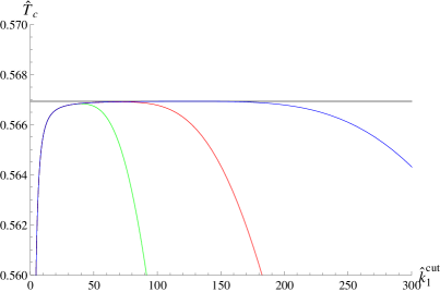
Figure 2: $\hat{T}_{c}$ as a function of $\hat{k}_{1}^{\text{cut}}$ (left panel) and $\hat{k}_{1}^{\text{cut}}/(N_{1}+1/2)$ (right panel) for $N_{1}=64$ (green curve), $N_{1}=128$ (red curve), and $N_{1}=256$ (blue curve) obtained from (III.3) with $N_{00}=256$ and $N_{0c}=36$ (the black lines indicate the infinite-volume continuum result $\hat{T}_{c}=e^{C}/\pi$).

• For sufficiently large $N_{1}$ and a suitably chosen $\hat{k}_{1}^{\text{cut}}$ the resulting $\hat{T}_{c}$ should be close to the analytically known infinite-volume continuum result $\hat{T}_{c}=e^{C}/\pi\approx 0.566$. Again one can observe plateau-like regions, where this is the case.

• For a small spatial momentum cutoff $\hat{k}_{1}^{\text{cut}}$ there are strong deviations (for small $\hat{k}_{1}^{\text{cut}}$, curves obtained with different $N_{1}$ fall on top of each other, when plotted versus $\hat{k}_{1}^{\text{cut}}$).

• For $\hat{k}_{1}^{\text{cut}}/(N_{1}+1/2)\raisebox{-2.15277pt}{$\,\stackrel{{\scriptstyle>}}{{\scriptstyle\sim}}\,$}1.0$ there are also strong deviations, because the extent of the periodic spatial dimension $\hat{L}_{1}=2\pi(N_{1}+1/2)/\hat{k}_{1}^{\text{cut}}$ is quite small and, therefore, a poor approximation for infinitely extended space (for $\hat{k}_{1}^{\text{cut}}/(N_{1}+1/2)\raisebox{-2.15277pt}{$\,\stackrel{{\scriptstyle>}}{{\scriptstyle\sim}}\,$}1.0$, curves obtained with different $N_{1}$ fall on top of each other, when plotted versus $\hat{k}_{1}^{\text{cut}}/(N_{1}+1/2)\propto 1/\hat{L}_{1}$).

In other words, to obtain accurate results, $1\ll\hat{k}_{1}^{\text{cut}}\ll N_{1}$ has to be fulfilled, which is only possible, if a sufficiently large number of spatial modes $N_{1}$ is used. According to the definition (35) the optimal $\hat{k}_{1}^{\text{cut}}$ for given $N_{1}$ is the maximum of the corresponding curves in FIG. 2.

In TABLE 2 one can see the accuracy $1-\hat{T}_{c}/(e^{C}/\pi)$ of the numerically obtained $\hat{T}_{c}$ for various values of $N_{1}$, again for $N_{00}=256$ and the corresponding optimal $N_{0c}=36$. Note that errors due to the finite-mode regularization in temporal direction and in spatial direction have opposite sign (cf. FIG. 1 and FIG. 2). Consequently, one obtains the most accurate result for $\hat{T}_{c}$ not for $N_{1}\rightarrow\infty$, but when both errors almost cancel each other. This is the case for $N_{1}=249$, i.e., for $N_{1}$ similar to $N_{00}$ (for a more detailed discussion cf. Sec. III.3.3). Also listed in TABLE 2 are the spatial momentum cutoff $\hat{k}_{1}^{\text{cut,opt}}$ and the corresponding spatial extension $\hat{L}_{1}^{\text{opt}}=2\pi(N_{1}+1/2)/\hat{k}_{1}^{\text{cut,opt}}$. Again, when increasing $N_{1}$, there is a similar increase in the spatial momentum cutoff $\hat{k}_{1}^{\text{cut,opt}}$, but only a slight increase in the spatial extension $\hat{L}_{1}^{\text{opt}}$ approximating infinite volume. As already mentioned this is typical for lattice calculations, where cutoff effects are only polynomially suppressed, while finite-volume effects are exponentially suppressed.

$N_{1}$	$1-\hat{T}_{c}/(e^{C}/\pi)$	$\hat{k}_{1}^{\text{cut,opt}}$	$\hat{L}_{1}^{\text{opt}}$
$32$	$+5.789\cdot 10^{-4}$	$2.273\cdot 10^{1}$	$\phantom{0}8.99$
$64$	$+1.766\cdot 10^{-4}$	$3.991\cdot 10^{1}$	$10.15$
$128$	$+4.324\cdot 10^{-5}$	$7.138\cdot 10^{1}$	$11.31$
$249$	$-2.720\cdot 10^{-8}$	$1.261\cdot 10^{2}$	$12.43$
$256$	$-1.003\cdot 10^{-6}$	$1.291\cdot 10^{2}$	$12.48$
$512$	$-1.460\cdot 10^{-5}$	$2.329\cdot 10^{2}$	$13.83$
$1024$	$-1.798\cdot 10^{-5}$	$4.179\cdot 10^{2}$	$15.41$
$2048$	$-1.871\cdot 10^{-5}$	$7.616\cdot 10^{2}$	$16.90$
$4096$	$-1.882\cdot 10^{-5}$	$1.403\cdot 10^{3}$	$18.35$

Table 2: Accuracy of the numerically obtained $\hat{T}_{c}$ for $N_{00}=256$, $N_{0c}=36$, and various values of $N_{1}$.

III.3.3 Optimizing the ratio of $N_{00}$ and $N_{1}$

As already mentioned the maximum number of modes $\propto N_{00}N_{1}$ is limited by the available computer resources. In the previous subsection it has been observed that for $N_{00}=256$ and $N_{1}=249$ the errors in $\hat{T}_{c}$ due to the finite-mode regularization almost cancel. Also for other choices of $N_{00}$ such a nearly perfect cancellation is present for $N_{1}\approx N_{00}$, as collected in TABLE 3. Moreover, note that the temporal momentum cutoff $\hat{k}_{0}^{\text{cut,opt}}$ and the spatial momentum cutoff $\hat{k}_{1}^{\text{cut,opt}}$ are close to each other.

Similarly, in FIG. 3 we compare the numerically obtained $\hat{T}_{c}$ for various $N_{00}$ and $N_{1}$ with the infinite-volume continuum result $\hat{T}_{c}=e^{C}/\pi$. The figure suggests choosing $N_{00}=N_{1}$ as a simple rule, which obviously leads to very accurate numerical results (the black filled circles in FIG. 3). Unless mentioned otherwise, we will use $N_{00}=N_{1}$ in the following. Of course, such a cancellation of errors might not occur for quantities other than $\hat{T}_{c}$. Moreover, when considering also the possibility of an inhomogeneous condensate, as we will do in Sec. III.4, it could be necessary to have a finer resolution or a larger extent of the spatial dimension, which might require a rather large $N_{1}\gg N_{00}$.

$N_{00}$	$N_{1}$	$N_{0c}^{\text{opt}}$	$\hat{k}_{0}^{\text{cut,opt}}$	$\hat{k}_{1}^{\text{cut,opt}}$
$32$	$30$	$6$	$2.137\cdot 10^{1}$	$2.190\cdot 10^{1}$
$64$	$62$	$11$	$3.919\cdot 10^{1}$	$3.932\cdot 10^{1}$
$128$	$125$	$20$	$7.124\cdot 10^{1}$	$7.034\cdot 10^{1}$
$256$	$249$	$36$	$1.282\cdot 10^{2}$	$1.261\cdot 10^{2}$
$512$	$497$	$66$	$2.351\cdot 10^{2}$	$2.287\cdot 10^{2}$
$1024$	$994$	$121$	$4.310\cdot 10^{2}$	$4.188\cdot 10^{2}$
$2048$	$1985$	$223$	$7.844\cdot 10^{2}$	$7.710\cdot 10^{2}$
$4096$	$3966$	$414$	$1.475\cdot 10^{3}$	$1.428\cdot 10^{3}$

Table 3: Pairs $N_{00}$ and $N_{1}$, where the errors due to the finite-mode regularization for $\hat{T}_{c}$ almost cancel, and the corresponding $N_{0c}^{\text{opt}}$, $\hat{k}_{0}^{\text{cut,opt}}$, and $\hat{k}_{1}^{\text{cut,opt}}$.

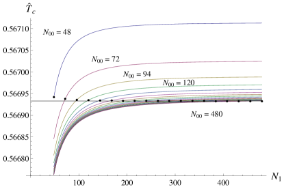
Figure 3: $\hat{T}_{c}$ as a function of $N_{1}$ for several $N_{00}$ (filled black circles indicate symmetric choices $N_{00}=N_{1}$, the black line is the infinite-volume continuum result $\hat{T}_{c}=e^{C}/\pi$).

III.3.4 Summary

Based on these investigations we propose and adopt the following strategy to determine the parameters $N_{0c}$, $N_{1}$, $\hat{k}_{0}^{\text{cut}}$, $\hat{k}_{1}^{\text{cut}}$, and $\lambda$:

• Use $N_{00}=N_{1}$ as large as possible (limited by the available computer resources).

• Determine the corresponding optimal $N_{0c}$ from a computation in the limit $N_{1}\rightarrow\infty$ and $\hat{k}_{1}^{\text{cut}}\rightarrow\infty$ as described in Sec. III.3.1 (cf. also TABLE 1, third column). This computation also provides a value for $\hat{k}_{0}^{\text{cut}}$ (TABLE 1, fifth column), which is a good approximation for $\hat{k}_{0}^{\text{cut}}$ at finite, but large $N_{1}$ and $\hat{k}_{1}^{\text{cut}}$. Assign this value to $\hat{k}_{1}^{\text{cut}}$ (cf. Sec. III.3.3).

• Solve Eq. (III.3) to determine $\hat{k}_{0}^{\text{cut}}$ (now for finite $N_{1}$ and $\hat{k}_{1}^{\text{cut}}$) for the previously chosen $N_{00}$ and $N_{1}$ [step (1)] and $N_{0c}$ and $\hat{k}_{1}^{\text{cut}}$ [step (2)].

• Determine $\lambda$ via Eq. (29) [or equivalently via Eq. (30)].

For all further computations, e.g. when computing the phase diagram for a homogeneous condensate $\sigma=\text{constant}$ or an inhomogeneous condensate $\sigma=\sigma(x_{1})$, the parameters $N_{1}$, $\hat{k}_{0}^{\text{cut}}$, $\hat{k}_{1}^{\text{cut}}$, and $\lambda$ are not changed anymore. The temperature $\hat{T}=1/\hat{L}_{0}=\hat{k}_{0}^{\text{cut}}/2\pi N_{0}$ can be adjusted by using different numbers of temporal modes $N_{0}$. $N_{0c}$ corresponds to the critical temperature $\hat{T}_{c}$.

III.4 Computation of the phase diagram for a homogeneous condensate $\sigma=\text{constant}$

To determine the phase diagram for a homogeneous condensate, i.e., $\sigma$ as a function of the chemical potential $\mu$ and the temperature $T$, one proceeds as in the previous subsection. From

$$0=\frac{d}{d\hat{\sigma}}\frac{S_{E,\text{eff}}(\hat{\sigma})}{N}$$ (36)

one can derive the generalization of Eq. (28) for arbitrary $\mu\geq 0$,

$$0=\frac{2\pi^{2}N_{0}(N_{1}+1/2)}{\lambda\hat{k}_{0}^{\text{cut}}\hat{k}_{1}^{\text{cut}}}-2\sum_{n_{0}=1}^{N_{0}}\sum_{n_{1}=-N_{1}}^{N_{1}}\frac{\bigg{(}\hat{k}_{0}^{\text{cut}}\frac{n_{0}-1/2}{N_{0}}\bigg{)}^{2}+\bigg{(}\hat{k}_{1}^{\text{cut}}\frac{n_{1}}{N_{1}+1/2}\bigg{)}^{2}+\hat{\sigma}^{2}-\hat{\mu}^{2}}{\bigg{[}\bigg{(}\hat{k}_{0}^{\text{cut}}\frac{n_{0}-1/2}{N_{0}}\bigg{)}^{2}+\bigg{(}\hat{k}_{1}^{\text{cut}}\frac{n_{1}}{N_{1}+1/2}\bigg{)}^{2}+\hat{\sigma}^{2}-\hat{\mu}^{2}\bigg{]}^{2}+\bigg{(}2\hat{\mu}\hat{k}_{0}^{\text{cut}}\frac{n_{0}-1/2}{N_{0}}\bigg{)}^{2}}\;.$$ (37)

If this equation has a solution $\hat{\sigma}^{2}=A>0$ for given $(\hat{\mu},\hat{T})$, and if $S_{E,\text{eff}}(\sqrt{A})<S_{E,\text{eff}}(0)$, this solution is the value of the chiral condensate, i.e., $\hat{\sigma}=\pm\sqrt{A}$, and $(\hat{\mu},\hat{T})$ is inside the chirally broken phase. If there is no such solution, or if $S_{E,\text{eff}}(\sqrt{A})\geq S_{E,\text{eff}}(0)$, then $\hat{\sigma}=0$ and $(\hat{\mu},\hat{T})$ is a point inside the chirally symmetric phase or on the phase boundary.

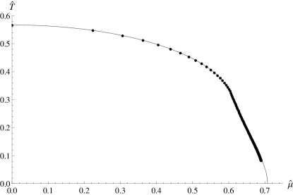
Figure 4: Phase diagram of the GN model for a homogeneous condensate $\sigma=\text{constant}$ for $N_{00}=N_{1}=192$ [the light gray curve is the infinite-volume continuum result Wolff:1985av ].

The phase diagram for a homogeneous condensate obtained with $N_{00}=N_{1}=192$ (with corresponding $N_{0c}=28$, $\hat{k}_{0}^{\text{cut}}=9.974\cdot 10^{1}$, $\hat{k}_{1}^{\text{cut}}=1.011\cdot 10^{2}$ and $\lambda=0.3328$) is shown in FIG. 4. It is in excellent agreement with the infinite-volume continuum result Wolff:1985av .

III.5 Finite-mode regularization, spatially inhomogeneous condensate $\sigma=\sigma(x_{1})$

To study the possibility of a spatially inhomogeneous condensate, $\hat{\sigma}$ is written as a superposition of a finite number of plane waves,

$$\hat{\sigma}(\hat{x}_{1})=\frac{\sigma(x_{1})}{\sigma_{0}}=\sum_{m=-M}^{M}c_{m}\frac{e^{-\imath\hat{p}\hat{x}_{1}}}{\sqrt{\hat{L}_{1}}}\quad,\quad\hat{p}=\frac{2\pi}{\hat{L}_{1}}m\quad,\quad c_{+m}=(c_{-m})^{\ast},$$ (38)

as done in Eqs. (22) and (23) for the fermionic fields $\hat{\psi}_{j}$. The resolution of $\hat{\sigma}$ should be coarser than the resolution of $\hat{\psi}_{j}$, i.e., $M\ll N_{1}$, to obtain stable and meaningful numerical results [cf. Ref. Wagner:2007he for a detailed discussion].

In the case of a spatially inhomogeneous condensate plane waves are no longer eigenfunctions of the Dirac operator $Q$. Consequently, $\ln[\det(\hat{Q}^{\dagger}\hat{Q})]$ cannot be expressed as a product over modes as done in Eq. (III.2). One has to represent $\hat{Q}^{\dagger}\hat{Q}$ as a matrix, where the rows and columns correspond to the plane-wave basis functions of the fermionic fields $e^{\mp\imath(\hat{k}_{0}\hat{x}_{0}+\hat{k}_{1}\hat{x}_{1})}/\sqrt{\hat{L}_{0}\hat{L}_{1}}$ [cf. Eqs. (22) and (23)],

$$\langle\hat{k}_{0},\hat{k}_{1}|\hat{Q}^{\dagger}\hat{Q}|\hat{k}_{0}^{\prime},\hat{k}_{1}^{\prime}\rangle=$$

$$\hskip 14.22636pt=\frac{1}{\hat{L}_{0}\hat{L}_{1}}\int_{0}^{\hat{L}_{0}}d\hat{x}_{0}\,\int_{0}^{\hat{L}_{1}}d\hat{x}_{1}\,e^{+\imath(\hat{k}_{0}\hat{x}_{0}+\hat{k}_{1}\hat{x}_{1})}\bigg{(}-\gamma_{\mu}\hat{\partial}_{\mu}+\gamma_{0}\hat{\mu}+\sum_{m=-M}^{+M}c_{m}\frac{e^{-\imath\hat{p}\hat{x}_{1}}}{\sqrt{\hat{L}_{1}}}\bigg{)}$$

$$\hskip 28.45274pt\times\bigg{(}+\gamma_{\mu}\hat{\partial}_{\mu}+\gamma_{0}\hat{\mu}+\sum_{m^{\prime}=-M}^{+M}c_{m^{\prime}}\frac{e^{-\imath\hat{p}^{\prime}\hat{x}_{1}}}{\sqrt{\hat{L}_{1}}}\bigg{)}e^{-\imath(\hat{k}_{0}^{\prime}\hat{x}_{0}+\hat{k}_{1}^{\prime}\hat{x}_{1})}$$

$$\hskip 14.22636pt=\frac{\delta_{\hat{k}_{0},\hat{k}_{0}^{\prime}}}{\hat{L}_{1}}\int_{0}^{\hat{L}_{1}}d\hat{x}_{1}\,e^{+\imath\hat{k}_{1}\hat{x}_{1}}\bigg{(}+\imath\gamma_{0}\hat{k}_{0}+\imath\gamma_{1}\hat{k}_{1}+\gamma_{0}\hat{\mu}+\sum_{m=-M}^{+M}c_{m}\frac{e^{-\imath\hat{p}\hat{x}_{1}}}{\sqrt{\hat{L}_{1}}}\bigg{)}$$

$$\hskip 28.45274pt\times\bigg{(}-\imath\gamma_{0}\hat{k}_{0}^{\prime}-\imath\gamma_{1}\hat{k}_{1}^{\prime}+\gamma_{0}\hat{\mu}+\sum_{m^{\prime}=-M}^{+M}c_{m^{\prime}}\frac{e^{-\imath\hat{p}^{\prime}\hat{x}_{1}}}{\sqrt{\hat{L}_{1}}}\bigg{)}e^{-\imath\hat{k}_{1}^{\prime}\hat{x}_{1}}$$ (39)

with $\hat{p}=2\pi m/\hat{L}_{1}$ and $\hat{p}^{\prime}=2\pi m^{\prime}/\hat{L}_{1}$. These matrix elements can be calculated analytically. Note that this matrix representation of $\det(\hat{Q}^{\dagger}\hat{Q})$ has a block-diagonal structure with $2N_{0}$ blocks of size $2(2N_{1}+1)$ (the blocks are labeled by $\hat{k}_{0}=\hat{k}_{0}^{\prime}$; the rows and columns of each block correspond to the spatial momenta $\hat{k}_{1}$ and $\hat{k}_{1}^{\prime}$ and the two spin components). $\ln[\det(\hat{Q}^{\dagger}\hat{Q})]$ is then the sum over $\ln[\det(\ldots)]$ of the blocks, where each term of that sum can be evaluated numerically e.g. by means of an LU decomposition.

III.6 Computation of the phase diagram for an inhomogeneous condensate $\sigma=\sigma(x_{1})$

When allowing for a spatially inhomogeneous condensate $\sigma=\sigma(x_{1})$, there are three phases:

• For small chemical potential $\hat{\mu}$ and low temperature $\hat{T}$ chiral symmetry is broken by a homogeneous condensate $\hat{\sigma}=\text{constant}\neq 0$ [corresponding to $c_{0}\neq 0$, $c_{m}=0$ for $m\neq 0$ in Eq. (38)].

• For high temperature $\hat{T}$ chiral symmetry is intact and $\hat{\sigma}=0$ [corresponding to $c_{m}=0$ for all $m$ in Eq. (38)].

• For large chemical potential $\hat{\mu}$ and low temperature $\hat{T}$ there is a spatially inhomogeneous condensate $\hat{\sigma}=\hat{\sigma}(\hat{x}_{1})$ [corresponding to $c_{m}\neq 0$ for at least one $m\neq 0$ in Eq. (38)].

The phase diagram for a spatially inhomogeneous condensate obtained with $N_{00}=N_{1}=192$ and $M=10$ (with corresponding $N_{0c}=28$, $\hat{k}_{0}^{\text{cut}}=9.974\cdot 10^{1}$, $\hat{k}_{1}^{\text{cut}}=1.011\cdot 10^{2}$ and $\lambda=0.3328$) is shown in FIG. 5. It is in excellent agreement with the infinite-volume continuum result Thies:2003kk ; Schnetz:2004vr .

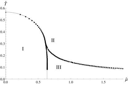
Figure 5: Phase diagram of the GN model for a spatially inhomogeneous condensate $\sigma=\sigma(x_{1})$ for $N_{00}=N_{1}=192$ and $M=10$ [the light gray curve is the infinite-volume continuum result Thies:2003kk ; Schnetz:2004vr ].

The numerical determination of the phase boundaries is discussed in detail in Ref. Wagner:2007he and, therefore, only summarized briefly in the following.

• Phase boundary I-II:
  The phase boundary between $\hat{\sigma}=\text{constant}\neq 0$ (phase I) and $\hat{\sigma}=0$ (phase II) can be determined as explained in Sec. III.4 for the phase diagram for a homogeneous condensate.

• Phase boundary I-III:
  To determine the phase boundary between $\hat{\sigma}=\text{constant}\neq 0$ (phase I) and the inhomogeneous crystal phase (phase III), one again has to find the minimum of $S_{E,\text{eff}}/N$ with respect to $\hat{\sigma}$ as a function of $(\hat{\mu},\hat{T})$. This time, however, $\hat{\sigma}$ is not a constant, but a superposition of plane waves [cf. Eq. (38)]. The minimization has to be done with respect to the coefficients $c_{n}$.

• Phase boundary II-III:
  To determine the phase boundary between $\hat{\sigma}=0$ (phase II) and the inhomogeneous crystal phase (phase III), one can in principle proceed as for the phase boundary I-III. Note, however, that inside the crystal phase in the vicinity of the phase boundary I-III the constant $\hat{\sigma}$ of the phase diagram for a homogeneous condensate is a local minimum (the corresponding phase transition is of first order), while in the vicinity of the phase boundary II-III it is a saddle point (the corresponding phase transition is of second order). Therefore, a computationally simpler and cheaper way to determine the phase boundary II-III is to study the smallest eigenvalue of the Hessian matrix

  $$H_{mm^{\prime}}=\frac{\partial}{\partial C_{m}}\frac{\partial}{\partial C_{m^{\prime}}}\frac{S_{E,\text{eff}}(\hat{\sigma})}{N}\bigg{|}_{\hat{\sigma}=0}\quad,\quad C_{2m}=\text{Re}(c_{m})\quad,\quad C_{2m+1}=\text{Im}(c_{m})\;,$$ (40)

  with $0<m,m^{\prime}\leq M$. A negative eigenvalue amounts to a direction of negative curvature and, therefore, indicates the existence of an inhomogeneous condensate.

Since the finite-mode approach allows to determine the condensate $\sigma$ at given temperature $T$ for arbitrary chemical potential $\mu$, it is straightforward to study and reproduce the order of the transition along the phase boundaries I-II, I-III, and II-III.

IV Phase diagram of the $1+1$ dimensional $\chi$GN model

We proceed in the same way as explained in detail in the previous section for the GN model. After introducing two real scalar fields $\sigma$ and $\eta$, the partition function of the $\chi$GN model can be written as

$$Z=\int D\sigma\,D\eta\,e^{-S_{E,\text{eff}}[\sigma,\eta]}\quad,\quad S_{E,\text{eff}}[\sigma,\eta]=N\int d^{2}x\,\bigg{\{}\frac{1}{2\lambda}\Big{(}\sigma^{2}+\eta^{2}\Big{)}-\frac{1}{2}\ln[\det(Q^{\dagger}Q)]\bigg{\}}\;,$$ (41)

where

$$Q=\gamma_{\mu}\partial_{\mu}+\gamma_{0}\mu+\sigma+\eta\imath\gamma_{5}.$$

We then apply the finite-mode regularization, i.e., in analogy to Eq. (38) the scalar fields $\sigma$ and $\eta$ (the condensates) are represented as a sum over a finite number of modes,

$$\hat{\sigma}(\hat{x}_{1})=\frac{\sigma(x_{1})}{\Sigma_{0}}=\sum_{m=-M}^{M}c_{m}\frac{e^{-\imath\hat{p}\hat{x}_{1}}}{\sqrt{\hat{L}_{1}}}\quad,\quad c_{+m}=(c_{-m})^{\ast}\quad,$$ (42)

$$\hat{\eta}(\hat{x}_{1})=\frac{\eta(x_{1})}{\Sigma_{0}}=\sum_{m=-M}^{M}d_{m}\frac{e^{-\imath\hat{p}\hat{x}_{1}}}{\sqrt{\hat{L}_{1}}}\quad,\quad d_{+m}=(d_{-m})^{\ast}\quad,\quad\hat{p}=\frac{2\pi}{\hat{L}_{1}}m\;.$$ (43)

Similary, $Q^{\dagger}Q$ is written as a matrix, where the rows and columns correspond to plane-wave basis functions $e^{\mp\imath(\hat{k}_{0}\hat{x}_{0}+\hat{k}_{1}\hat{x}_{1})}/\sqrt{\hat{L}_{0}\hat{L}_{1}}$, [cf. Sec. III.5 and Eqs. (22) and (23) for details]. Since $S_{E,\text{eff}}$ is invariant under the transformation $(\sigma,\eta)\rightarrow R(\sigma,\eta)$ with $R\in\text{O(2)}$, dimensionful quantities are expressed in units of $\Sigma_{0}$, where

$$\Sigma_{0}=\Sigma\Big{|}_{T=0,\mu=0}\quad,\quad\Sigma=\Big{(}\sigma^{2}+\eta^{2}\Big{)}^{1/2}\;,$$ (44)

and denoted by a hat $\hat{\phantom{x}}$.

We have studied the phase diagram of the $\chi$GN model using $M=10$ modes for the condensates and $N_{00}=N_{1}=96$ modes for the fermionic determinant.

For temperatures $\hat{T}>\hat{T}_{c}=e^{C}/\pi$ and arbitrary chemical potential $\mu$ chiral symmetry is restored, i.e., the effective action (41) is minimized for $c_{j}=d_{j}=0$, which corresponds to vanishing condensates $\sigma=\eta=0$.

For $T<T_{c}$ we find several local minima of $S_{E,\text{eff}}$, which are given by $c_{m}=\pm id_{m}\neq 0$ for a single mode $m$, while $c_{j}=d_{j}=0$ for all other modes, i.e., $j\neq m$. The condensates $\sigma$ and $\eta$ are harmonic functions, i.e., CDWs, with the same amplitude, but with a relative phase shift $\pm\pi/2$, implying $\Sigma=\text{constant}$ [cf. Eq. (44)]. The minimal values of $S_{E,\text{eff}}$ are plotted in FIG. 6 as functions of the chemical potential $\mu$ for $m=0,1,2,3$ and two different temperatures $\hat{T}=0.378,0.189$ ($N_{0}=24,48$, while $N_{00}=N_{1}=96$ and $M=10$). For $\mu=0$ the absolute minimum of $S_{E,\text{eff}}$ corresponds to $m=0$, i.e., $\sigma,\eta=\text{const}$. The wavelength is proportional to $\mu$, i.e., for increasing $\mu$ the absolute minimum of $S_{E,\text{eff}}$ corresponds to larger and larger $m>0$. Two examples of the resulting CDWs ($\hat{T}=0.095<\hat{T}_{c}$ [$N_{0}=96$] and $\hat{\mu}=0.295,0.875$) are shown in FIG. 7.

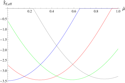
Figure 6: $\chi$GN model. Local minimal values of $S_{E,\text{eff}}$ as functions of the chemical potential $\mu$ for $m=0$ (blue), $m=1$ (red), $m=2$ (green) and $m=3$ (gray) and two different temperatures $\hat{T}=0.378$ ($N_{0}=24$, left panel) and $\hat{T}=0.189$ ($N_{0}=48$, right panel).

Figure 7: $\chi$GN model. Resulting chiral CDWs for $\hat{T}=0.095<\hat{T}_{c}$ ($N_{0}=96$) and $\hat{\mu}=0.295$ (left panel) and $\hat{\mu}=0.875$ (right panel).

The resulting phase diagram is, therefore, quite different from the phase diagram of the GN model: there are only two phases, for $T<T_{c}$ a CDW, and for $T>T_{c}$ chiral symmetry is restored. This is in agreement with analytically known results Schon:2000he ; Basar:2009fg .

V Phase diagram of the NJL₂ model

Again the technical steps needed to compute the phase diagram closely parallel those discussed for the GN model and the $\chi$GN model. This time four real scalar fields $\sigma$ and $\pi_{j}$, $j=1,2,3$ are required, where

$$Z=\int D\sigma\bigg{(}\prod_{j=1}^{3}D\pi_{j}\bigg{)}e^{-S_{E,\text{eff}}[\sigma,\pi_{j}]}\quad,\quad S_{E,\text{eff}}[\sigma,\pi_{j}]=N\int d^{2}x\,\bigg{\{}\frac{1}{2\lambda}\bigg{(}\sigma^{2}+\sum_{j=1}^{3}\pi_{j}^{2}\bigg{)}-\frac{1}{2}\ln[\det(Q^{\dagger}Q)]\bigg{\}}\;,$$ (45)

with

$$Q=\gamma_{\mu}\partial_{\mu}+\gamma_{0}\mu+\sigma+\imath\gamma_{5}\sum_{j=1}^{3}\tau_{j}\pi_{j}\;.$$ (46)

$\sigma$ and $\pi_{j}$ as well as $\det(Q^{\dagger}Q)$ are then finite-mode regularized as done in Eqs. (38), (42), and (43) and Sec. III.5, respectively. Due to the invariance of $S_{E,\text{eff}}$ with respect to $(\sigma,\pi_{1},\pi_{2},\pi_{3})\rightarrow R(\sigma,\pi_{1},\pi_{2},\pi_{3})$ with $R\in\text{O(4)}$, dimensionful quantities are expressed in units of

$$\Sigma_{0}=\Sigma\Big{|}_{T=0,\mu=0}\quad,\quad\Sigma=\bigg{(}\sigma^{2}+\sum_{j=1}^{3}\pi_{j}^{2}\bigg{)}^{1/2}\;,$$ (47)

and denoted by a hat $\hat{\phantom{x}}$.

We have studied the phase diagram of the NJL₂ model using $M=4$ modes for the condensates and $N_{00}=N_{1}=72$ modes for the fermionic determinant. For any temperature and chemical potential the four condensates are proportional to each other, i.e., $\sigma\propto\pi_{1}\propto\pi_{2}\propto\pi_{3}\propto\Sigma$ and also proportional to the chiral condensate $\sigma$ of the GN model. Consequently, we obtain exactly the same phase diagram for the NJL₂ model as for the GN model, which is shown in FIG. 5. These findings extend existing results, where only a CDW [$\sigma(x)\propto\cos(2bx)$ and $\pi_{3}(x)\propto\sin(2bx)$] has been considered Ebert:2011rg . Our results show that an inhomogeneous phase is indeed present at larger $\mu$ and not too large $T$. However, this inhomogeneous phase exhibits solitonic structures and not a CDW. This result is similar to those found for the NJL model in $3+1$ dimensions, as discussed e.g. in Sec. VI or Ref. Carignano:2011gr .

VI Phase diagram of the NJL model

We investigate the phase diagram of the NJL model at nonzero temperature and density under the assumption that only the chiral condensate $\sigma$ defined in Eq. (8) condenses. Thus, we do not take into account condensation of the pion-like field combinations $\bar{\psi}_{j,f}\vec{\tau}\imath\gamma_{5}\psi_{j,f}$ appearing e.g. in Eq. (6). The chiral condensate $\sigma$ is, in general, a function of the three spatial coordinates $\vec{x}=(x_{1},x_{2},x_{3})$, i.e., $\sigma=\sigma(\vec{x})$. However, previous investigations based on special ansätze have shown that modulations in more than one dimension are not favoured energetically Carignano:2014jla ; Buballa:2014tba . Thus, for the sake of simplicity in the following we assume that $\sigma$ depends only on one of the three spatial coordinates, e.g. $x_{3}$, i.e.,

$$\hat{\sigma}=\hat{\sigma}(\hat{x}_{3})=\frac{\sigma(x_{3})}{\sigma_{0}}=\sum_{m=-M}^{M}c_{m}\frac{e^{-\imath\hat{p}\hat{x}_{3}}}{\sqrt{\hat{L}_{3}}}\quad,\quad c_{+m}=(c_{-m})^{\ast}\quad,\quad\hat{p}=\frac{2\pi}{\hat{L}_{3}}m\;.$$ (48)

Of course, a study of the NJL model in the context of the finite-mode approach without this assumption is an interesting topic which we plan to investigate in the future.

Proceeding as in Sec. III.1 for the GN model we obtain the partition function of the NJL model in $3+1$ dimensions,

$$Z=\int D\sigma\,e^{-S_{E,\text{eff}}[\sigma]}\quad,\quad S_{E,\text{eff}}[\sigma]=N\int d^{4}x\,\bigg{\{}\frac{6G}{N^{2}}\sigma^{2}-\ln[\det(Q^{\dagger}Q)]\bigg{\}}\;,$$ (49)

where $Q=\gamma_{\mu}\partial_{\mu}+\gamma_{0}\mu+m_{0}^{\ast}$. The Pauli-Villars regularization can be implemented by adding heavy fermions as explained in Sec. II.2,

$$S_{E,\text{eff,PV}}[\sigma]=S_{E,\text{eff}}[\sigma]-N\int d^{4}x\,\sum_{k=1}^{N_{\mathrm{PV}}}C_{k}\ln[\det(\tilde{Q}_{k}^{\dagger}\tilde{Q}_{k})]\;,$$ (50)

with $\tilde{Q}_{k}=\gamma_{\mu}\partial_{\mu}+\gamma_{0}\mu+M_{k}.$

For a convenient comparison with the existing literature on the NJL model (and in contrast to the previous sections, where we discussed 1+1 dimensional models) we express our results in the following in units of GeV. To this end, the two parameters of the NJL model, the coupling constant $G$ and the Pauli-Villars energy scale $\Lambda_{\text{PV}}$, are fixed by requiring that a certain effective mass $m_{0}^{\ast}$ is realized (we perform computations for three different choices, $m_{0}^{\ast}\in\{250\,\text{MeV}\,,\,300\,\text{MeV}\,,\,350\,\text{MeV}\}$) and that the pion decay constant reproduces the correct value in the chiral limit, $f_{\pi}=88\,\text{MeV}$ Carignano:2011gr ; Nickel:2009wj . [For the evaluation of the pion decay constant in the framework of the NJL model, we refer to Ref. Klevansky:1992qe .]

The resulting phase diagrams for $N_{\text{PV}}=2$ additional heavy fermions, effective quark masses $m_{0}^{\ast}\in\{250\,\text{MeV}\,,\,300\,\text{MeV}\,,\,350\,\text{MeV}\}$ and $M=5$ and $N_{00}=N_{1}=120$ modes are shown in FIG. 8. The corresponding Pauli-Villars cutoffs are $\Lambda_{PV}\equiv\{736.8\,$MeV$,\,647.4\,$MeV$,\,608.7\,$MeV$\}$, the maximum momentum used in the expansion of the chiral condensate is approximately $(M/N)\hat{k}_{1}^{\text{cut}}\approx 650\,\text{MeV}$, where $\hat{k}_{1}^{\text{cut}}$ denotes the maximum momentum in the expansion of the fermionic fields, see Eq. (25).

Let us discuss the role of the two energy scales $\Lambda_{PV}$ and $\hat{k}_{1}^{\text{cut}}$ in somewhat greater detail. As mentioned already in Sec. II.B, the NJL model is non-renormalizable. As a consequence, the NJL model is only defined once the regularization has been fixed. Moreover, the corresponding energy scale (the Pauli-Villars cutoff $\Lambda_{PV}$ in our implementation of the NJL model) should be regarded as a physical parameter of the NJL model, with crucial impact on all physical quantities. On the other hand, our numerical approach contains also a cutoff due to the lattice regularization in momentum space, i.e., due to using a finite number of modes, see Eq. (25). The cutoff $\hat{k}_{1}^{\text{cut}}$ is purely technical and should be taken as large as possible. In particular, $\hat{k}_{1}^{\text{cut}}$ should be much larger than $\Lambda_{PV}.$ In the numerical calculations leading to Fig. 8 we have that $\hat{k}_{1}^{\text{cut}}/\Lambda_{PV}=25.4,$ thus $\hat{k}_{1}^{\text{cut}}$ is about $16$ GeV. This is indeed a very large value that assures that for all practical purposes the results do not depend on $\hat{k}_{1}^{\text{cut}}$. Such a high value also assures that the continent of Fig. 8 is not an artifact of our numerical calculation. We have also verified that relevant quantities, such as the critical temperature, do not depend on $\hat{k}_{1}^{\text{cut}}$ once it is chosen sufficiently large.

Quite remarkably, these phase diagrams are similar to that obtained for the 1+1 dimensional GN model (cf. FIG. 5). This result suggests that the 3+1 dimensional NJL model, which represents a non-renormalizable, but in many aspects realistic chiral model of QCD, generates a phase diagram whose most salient features can be understood in a simpler 1+1 dimensional field theory. However, it should also be stressed that this result is obtained in the specific case of the Pauli-Villars regularization and that the existence of an inhomogeneous condensate depends on the chosen regularization scheme.

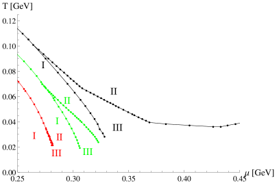
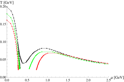
Figure 8: Phase diagram of the NJL model for a spatially inhomogeneous condensate $\sigma=\sigma(x_{3})$ for $N_{\text{PV}}=2$, $M=5$, $N_{00}=N_{1}=120$ and three different effective quark masses $m_{0}^{\ast}=250$ (red), $m_{0}^{\ast}=300$ (green) and $m_{0}^{\ast}=350\,\text{MeV}$ (black). There are three phases: (I) a homogeneous chirally broken phase $\sigma=\text{constant}\neq 0$, (II) a chirally restored phase $\sigma=0$, (III) an inhomogeneous phase (the left panel is a zoomed version of the right panel).

Independent of the concrete choice of the effective quark mass $m_{0}^{\ast}$ there is an inhomogeneous phase for large chemical potential $\mu$ and small temperature $T$, termed “continent” in Ref. Carignano:2011gr . However, at smaller $\mu$ the detailed shape of the phase diagram depends on the value of the effective quark mass. While at small $m_{0}^{\ast}$ an inhomogeneous “island” may be separated from the “continent”, at larger $m_{0}^{\ast}$ the island and the continent merge. Note that our results in the region $\mu<0.4\,\text{GeV}$ are in agreement with the findings of Ref. Nickel:2009wj . At somewhat larger $\mu$ they agree with the results of Ref. Carignano:2011gr , although the outlines of the continent were not traced to very large $\mu$ in that work. We find that, at even larger values of $\mu$, the transition temperature between the chirally restored and the inhomogeneous phase decreases with $\mu$, which is similar to the GN model.

We have repeated the study of the phase diagram of the NJL model for different volumes and verified that the results are very stable upon changing the volume. In particular, the form of the continent remains practically unchanged when $N_{00}$ is modified. We have checked the cases $N_{00}=N_{1}=48,$ $72,$ $96,120$ and already for $N_{00}=N_{1}=48$ the curves look just as in Figs. 8 and 9. We have then selected for the plots the highest number of modes ($N_{00}=N_{1}=120$) with which we could perform our numerical study in a reasonable computational time.

We have also compared regularizations using $N_{\text{PV}}=2$ and $N_{\text{PV}}=3$ additional heavy fermions (cf. FIG. 9). The effect of $N_{\text{PV}}$ on the shape of the phase diagram is rather mild: at intermediate chemical potential $\mu$ and temperature $T$ the inhomogeneous continent becomes somewhat larger when using a larger number of regulators.

Although a detailed study of the order of phase transitions at the phase boundaries is in principle straightforward, it would require a substantial numerical effort, especially in the case of a second-order phase transition, as expected for instance at the II-III boundary. We have, however, verified that $\left\langle\hat{\sigma}^{2}\right\rangle$ smoothly approaches zero at the II-III boundary. On the other hand, for small and constant temperature, $\left\langle\hat{\sigma}^{2}\right\rangle$ is a slowly decreasing function of the chemical potential $\mu.$

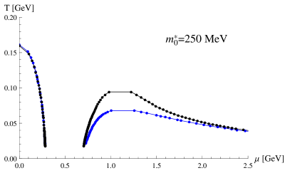
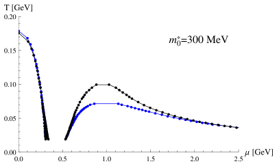
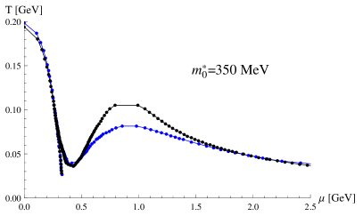
Figure 9: Phase diagram of the NJL model for a spatially inhomogeneous condensate for $N_{\text{PV}}=2$ (blue) and $N_{\text{PV}}=3$ (black) (further parameters chosen as in FIG. 8).

VII Summary and outlook

In this work we have used the finite-mode approach to investigate numerically the emergence of inhomogeneous chiral condensation in effective quark models in $1+1$ and $3+1$ dimensions. The main aim has been the determination of inhomogeneous condensation in QCD-inspired models without using a specific ansatz.

We have shown that our method accurately reproduces well-known analytical results concerning the phase diagram and the inhomogeneous condensation of $1+1$ dimensional models, in particular the Gross-Neveu and chiral Gross-Neveu model. By applying the approach to the NJL model in $3+1$ dimensions we could reproduce previous results based on specific ansätze for small chemical potential. In addition to that we were able to show that the inhomogeneous continent of Ref. Carignano:2011gr extends to very high densities, but not to arbitrarily large temperatures. Due to the fact that our results for the NJL phase diagram differ from previous ones at high density, it would be an interesting task for future studies to confirm or to falsify the presence of the continent using different approaches.

It is interesting to note that the GN model and the NJL₂ model have the same phase diagram, which in turn is also very similar to the NJL model in 1+3 dimensions. On the contrary, the phase diagram of the $\chi$GN model is completely different, showing that a different flavor structure has an impact on the phase diagram.

Our approach following Refs. Wagner:2007he ; Wagner:2007av is based on expanding fermionic fields and condensates in terms of plane waves. In this respect it is quite similar to existing general methods to compute inhomogeneous condensates Nickel:2008ng ; Carignano:2012sx ; Cao:2015rea . In other aspects it is, however, quite different. For example our method is based on a minimization of the effective action, not the Hamiltonian. A detailed and direct comparison regarding the computational efficiency of our method and those discussed in Refs. Nickel:2008ng ; Carignano:2012sx ; Cao:2015rea is difficult and would require computations of the same quantities within the same model using both types of methods. Since the basic idea of expanding in terms of plane waves is the same, we expect both types of methods to perform on a quantitatively similar level. Therefore, further studies would be necessary to clarify why the shape of the “continent” (see Fig. 9) looks different in the two methods.

Note that within our approach it is straightforward to replace the plane waves by another set of basis functions, as discussed and numerically demonstrated in Refs. Wagner:2007he ; Wagner:2007av . A first and straightforward step would be to still use a plane-wave expansion for the condensate, but to focus exclusively on higher modes in regions where the condensate is expected to exhibit strong oscillations (typically in inhomogeneous regions at large chemical potential $\mu$). Using a small number of modes with suitably chosen wave number might allow to explore the phase diagram quite extensively at rather moderate computational cost. The choice of the wave numbers could even be automated, i.e., included in the minimization procedure for the effective action. Another possibility within our numerical framework is to study specific ansätze to identify a small set of highly relevant degrees of freedom. This could not only provide certain physical insights, but also reduce the computing time significantly. The latter might be of particular importance, when studying two- or three-dimensional variations of the condensates.

In the future one could also apply the finite-mode approach to study the phase diagram of purely hadronic theories such as the extended Linear Sigma Model Parganlija:2012fy ; Gallas:2009qp . This approach is capable to correctly describe the vacuum phenomenology as well as the nuclear matter ground state properties Gallas:2011qp . As already shown in Ref. Heinz:2013hza , an inhomogeneous condensate in the form of a chiral density wave is favored with respect to a constant condensate at high density ($\gtrsim 2\rho_{0}$, where $\rho_{0}$ is the nuclear saturation density). It is an open question whether other structures minimize the effective potential even further. More generally, one could also apply the finite-mode approach to quark-based sigma models, e.g. Refs. Kovacs:2015vva ; Tawfik:2014gga .

Other interesting projects are the study of higher-dimensional modulations beyond the ansatz used in Ref. Carignano:2012sx and, since there is also no limitation in the number of inhomogeneous fields in the finite-mode approach, the study of interweaving chiral spirals Kojo:2011cn . Further effects at high densities such as inhomogeneous diquark condensation in $1+1$ as well as $3+1$ dimensions can also be taken into account Ebert:2014woa . Moreover, the models that we have studied were investigated in the chiral limit only. Future work could thus include a non-zero bare quark mass into the effective approaches.

References

- (1) U. G. Meissner, Phys. Rept. 161, 213 (1988).
- (2) P. Ko and S. Rudaz, Phys. Rev. D 50, 6877 (1994).
- (3) M. Urban, M. Buballa and J. Wambach, Nucl. Phys. A 697, 338 (2002) [hep-ph/0102260].
- (4) S. Gallas, F. Giacosa and D. H. Rischke, Phys. Rev. D 82 (2010) 014004 [arXiv:0907.5084 [hep-ph]]; S. Gallas and F. Giacosa, Int. J. Mod. Phys. A 29, no. 17, 1450098 (2014) [arXiv:1308.4817 [hep-ph]].
- (5) D. Parganlija, P. Kovacs, G. Wolf, F. Giacosa and D. H. Rischke, Phys. Rev. D 87, no. 1, 014011 (2013) [arXiv:1208.0585 [hep-ph]]; D. Parganlija, F. Giacosa and D. H. Rischke, Phys. Rev. D 82 (2010) 054024 [arXiv:1003.4934 [hep-ph]]; S. Janowski, F. Giacosa and D. H. Rischke, Phys. Rev. D 90 (2014) 11, 114005 [arXiv:1408.4921 [hep-ph]].
- (6) Y. Nambu and G. Jona-Lasinio, Phys. Rev. 122, 345 (1961).
- (7) Y. Nambu and G. Jona-Lasinio, Phys. Rev. 124, 246 (1961).
- (8) S. P. Klevansky, Rev. Mod. Phys. 64, 649 (1992).
- (9) U. Vogl and W. Weise, Prog. Part. Nucl. Phys. 27, 195 (1991).
- (10) T. Hatsuda and T. Kunihiro, Phys. Rept. 247, 221 (1994) [hep-ph/9401310].
- (11) M. Buballa, Phys. Rept. 407, 205 (2005) [hep-ph/0402234].
- (12) D. J. Gross and A. Neveu, Phys. Rev. D 10, 3235 (1974).
- (13) E. van Beveren, F. Kleefeld, G. Rupp and M. D. Scadron, , Mod. Phys. Lett. A 17, 1673 (2002) [hep-ph/0204139].
- (14) B. J. Schaefer, J. M. Pawlowski and J. Wambach, Phys. Rev. D 76, 074023 (2007) [arXiv:0704.3234 [hep-ph]].
- (15) G. Baym, Phys. Rev. Lett. 30, 1340 (1973).
- (16) R. F. Sawyer and D. J. Scalapino, Phys. Rev. D 7, 953 (1973).
- (17) D. K. Campbell, R. F. Dashen and J. T. Manassah, Phys. Rev. D 12, 979 (1975).
- (18) D. K. Campbell, R. F. Dashen and J. T. Manassah, Phys. Rev. D 12, 1010 (1975).
- (19) R. F. Dashen and J. T. Manassah, Phys. Lett. B 50, 460 (1974).
- (20) G. Baym, D. Campbell, R. F. Dashen and J. Manassah, Phys. Lett. B 58, 304 (1975).
- (21) A. B. Migdal, Rev. Mod. Phys. 50, 107 (1978).
- (22) G. Baym, Nucl. Phys. A 352, 355 (1981).
- (23) W. H. Dickhoff, A. Faessler, H. Muther and J. Meyer-Ter-Vehn, Nucl. Phys. A 368 (1981) 445.
- (24) K. Kolehmainen and G. Baym, Nucl. Phys. A 382, 528 (1982).
- (25) G. Baym, B. L. Friman and G. Grinstein, Nucl. Phys. B 210, 193 (1982).
- (26) A. Akmal and V. R. Pandharipande, Phys. Rev. C 56, 2261 (1997) [nucl-th/9705013].
- (27) A. Heinz, F. Giacosa and D. H. Rischke, Nucl. Phys. A 933, 34 (2015) [arXiv:1312.3244 [nucl-th]].
- (28) W. Broniowski and M. Kutschera, Phys. Lett. B 234, 449 (1990).
- (29) M. Sadzikowski and W. Broniowski, Phys. Lett. B 488, 63 (2000) [hep-ph/0003282].
- (30) R. Casalbuoni, R. Gatto, N. Ippolito, G. Nardulli and M. Ruggieri, Phys. Lett. B 627, 89 (2005) [Erratum-ibid. B 634, 565 (2006)] [hep-ph/0507247].
- (31) D. Nickel, Phys. Rev. D 80, 074025 (2009) [arXiv:0906.5295 [hep-ph]].
- (32) T. L. Partyka, Mod. Phys. Lett. A 26, 543 (2011) [arXiv:1005.2667 [hep-ph]].
- (33) W. Broniowski, Acta Phys. Polon. Supp. 5, 631 (2012) [arXiv:1110.4063 [nucl-th]].
- (34) S. Carignano and M. Buballa, Phys. Rev. D 86, 074018 (2012) [arXiv:1203.5343 [hep-ph]].
- (35) Y. -L. Ma, M. Harada, H. K. Lee, Y. Oh and M. Rho, Int. J. Mod. Phys. Conf. Ser. 29, 1460238 (2014) [arXiv:1312.2290 [hep-ph]].
- (36) M. Buballa and S. Carignano, Prog. Part. Nucl. Phys. 81 (2015) 39 [arXiv:1406.1367 [hep-ph]]. .
- (37) T. Kojo, Y. Hidaka, L. McLerran and R. D. Pisarski, Nucl. Phys. A 843, 37 (2010) [arXiv:0912.3800 [hep-ph]].
- (38) T. Kojo, Y. Hidaka, K. Fukushima, L. D. McLerran and R. D. Pisarski, Nucl. Phys. A 875, 94 (2012) [arXiv:1107.2124 [hep-ph]].
- (39) M. Harada, H. K. Lee, Y. L. Ma and M. Rho, arXiv:1502.02508 [hep-ph].
- (40) S. Carignano, D. Nickel and M. Buballa, Phys. Rev. D 82 (2010) 054009 [arXiv:1007.1397 [hep-ph]].
- (41) D. Müller, M. Buballa and J. Wambach, Phys. Lett. B 727 (2013) 240 [arXiv:1308.4303 [hep-ph]].
- (42) P. de Forcrand and U. Wenger, PoS LATTICE2006, 152 (2006) [hep-lat/0610117].
- (43) M. Wagner, Phys. Rev. D 76, 076002 (2007) [arXiv:0704.3023 [hep-lat]].
- (44) M. Wagner, PoS Lattice2007 339 (2007) [arXiv:0708.2359 [hep-lat]].
- (45) H. Abuki, D. Ishibashi and K. Suzuki, Phys. Rev. D 85, 074002 (2012) [arXiv:1109.1615 [hep-ph]].
- (46) D. Nickel and M. Buballa, Phys. Rev. D 79, 054009 (2009) [arXiv:0811.2400 [hep-ph]].
- (47) G. Cao, L. He and P. Zhuang, Phys. Rev. D 91, no. 11, 114021 (2015) [arXiv:1502.03392 [nucl-th]].
- (48) M. Thies and K. Urlichs, Phys. Rev. D 67, 125015 (2003) [hep-th/0302092].
- (49) G. Basar, G. V. Dunne and M. Thies, Phys. Rev. D 79, 105012 (2009) [arXiv:0903.1868 [hep-th]].
- (50) D. Ebert, T. G. Khunjua, K. G. Klimenko and V. C. .Zhukovsky, Phys. Rev. D 90, no. 4, 045021 (2014) [arXiv:1405.3789 [hep-th]].
- (51) T. Kojo, Phys. Rev. D 90, no. 6, 065030 (2014) [arXiv:1406.4630 [hep-ph]].
- (52) J. Braun, S. Finkbeiner, F. Karbstein and D. Roscher, arXiv:1410.8181 [hep-ph].
- (53) L. L. Salcedo, S. Levit and J. W. Negele, Nucl. Phys. B 361, 585 (1991).
- (54) R. F. Dashen, B. Hasslacher and A. Neveu, Phys. Rev. D 12, 2443 (1975).
- (55) D. Ebert and K. G. Klimenko, arXiv:0902.1861 [hep-ph].
- (56) L. McLerran and R. D. Pisarski, Nucl. Phys. A 796, 83 (2007) [arXiv:0706.2191 [hep-ph]].
- (57) L. McLerran, K. Redlich and C. Sasaki, Nucl. Phys. A 824, 86 (2009) [arXiv:0812.3585 [hep-ph]].
- (58) S. Carignano and M. Buballa, Acta Phys. Polon. Supp. 5, 641 (2012) [arXiv:1111.4400 [hep-ph]].
- (59) S. Carignano, M. Buballa and B. J. Schaefer, Phys. Rev. D 90 (2014) 1, 014033 [arXiv:1404.0057 [hep-ph]].
- (60) U. Wolff, Phys. Lett. B 157, 303 (1985).
- (61) G. ’t Hooft, Nucl. Phys. B 72, 461 (1974).
- (62) E. Witten, Nucl. Phys. B 160, 57 (1979).
- (63) R. F. Lebed, Czech. J. Phys. 49, 1273 (1999) [nucl-th/9810080].
- (64) O. Schnetz, M. Thies and K. Urlichs, Annals Phys. 321, 2604 (2006) [hep-th/0511206].
- (65) N. D. Mermin and H. Wagner, , Phys. Rev. Lett. 17, 1133 (1966).
- (66) S. R. Coleman, Commun. Math. Phys. 31 (1973) 259.
- (67) V. Schon and M. Thies, Phys. Rev. D 62, 096002 (2000) [hep-th/0003195].
- (68) V. Schon and M. Thies, In *Shifman, M. (ed.): At the frontier of particle physics, vol. 3* 1945-2032 [hep-th/0008175].
- (69) B. Bringoltz and M. Teper, Phys. Lett. B 628, 113 (2005) [hep-lat/0506034].
- (70) M. Panero, Phys. Rev. Lett. 103, 232001 (2009) [arXiv:0907.3719 [hep-lat]].
- (71) N. K. Glendenning, New York, USA: Springer 2nd ed. (2000) 492 p
- (72) I. Mishustin, J. Bondorf and M. Rho, Nucl. Phys. A 555, 215 (1993).
- (73) P. Papazoglou, S. Schramm, J. Schaffner-Bielich, H. Stoecker and W. Greiner, Phys. Rev. C 57, 2576 (1998) [nucl-th/9706024].
- (74) P. Papazoglou, D. Zschiesche, S. Schramm, J. Schaffner-Bielich, H. Stoecker and W. Greiner, Phys. Rev. C 59, 411 (1999) [nucl-th/9806087].
- (75) L. Bonanno, A. Drago and A. Lavagno, Phys. Rev. Lett. 99, 242301 (2007) [arXiv:0704.3707 [hep-ph]].
- (76) M. Buballa, private communication.
- (77) E. Nakano and T. Tatsumi, Phys. Rev. D 71 (2005) 114006 [hep-ph/0411350].
- (78) C. Itzykson and J.-B. Zuber, McGraw Hill 1980, Dover Publications (2006) 752 p.
- (79) A. A. Andrianov, L. Bonora and R. Gamboa-Saravi, Phys. Rev. D 26, 2821 (1982).
- (80) A. A. Andrianov and L. Bonora, Nucl. Phys. B 233, 232 (1984).
- (81) A. A. Andrianov and L. Bonora, Nucl. Phys. B 233, 247 (1984).
- (82) O. Schnetz, M. Thies and K. Urlichs, Annals Phys. 314, 425 (2004) [hep-th/0402014].
- (83) D. Ebert, N. V. Gubina, K. G. Klimenko, S. G. Kurbanov and V. C. Zhukovsky, Phys. Rev. D 84, 025004 (2011) [arXiv:1102.4079 [hep-ph]].
- (84) S. Gallas, F. Giacosa and G. Pagliara, Nucl. Phys. A 872 (2011) 13 [arXiv:1105.5003 [hep-ph]].
- (85) P. Kovács, Z. Szép and G. Wolf, J. Phys. Conf. Ser. 599 (2015) 1, 012010 [arXiv:1501.06426 [hep-ph]].
- (86) A. N. Tawfik and A. M. Diab, Phys. Rev. C 91 (2015) 1, 015204 [arXiv:1412.2395 [hep-ph]].
- (87) Let be an eigenfunction and be the corresponding eigenvalue of , i.e., . Then , i.e., the eigenvalues are either real or form complex conjugate pairs. Therefore, is real.