Collective excitations in Na₂IrO₃

Abstract

We study the collective excitations of Na₂IrO₃ in an itinerant electron approach. We consider a multi-orbital tight-binding model with the electron transfer between the Ir $5d$ states mediated via oxygen $2p$ states and the direct $d$-$d$ transfer on a honeycomb lattice. The one-electron energy as well as the ground state energy are investigated within the Hartree-Fock approximation. When the direct $d$-$d$ transfer is weak, we obtain nearly flat energy bands due to the formation of quasimolecular orbitals, and the ground state exhibits the zigzag spin order. The evaluation of the density-density correlation function within the random phase approximation shows that the collective excitations emerge as bound states. For an appropriate value of the direct $d$-$d$ transfer, some of them are concentrated in the energy region $\omega<$ 50 meV (magnetic excitations) while the others lie in the energy region $\omega>$ 350 meV (excitonic excitations). This behaviour is consistent with the resonant inelastic x-ray scattering spectra. We also show that the larger values of the direct $d$-$d$ transfer are unfavourable in order to explain the observed aspects of Na₂IrO₃ such as the ordering pattern of the ground state and the excitation spectrum. These findings may indicate that the direct $d$-$d$ transfer is suppressed by the structural distortions in the view of excitation spectroscopy, as having been pointed out in the ab initio calculation.

I Introduction

The physics of $5d$-based iridates has recently attracted much attention, since the competition between the large spin-orbit interaction (SOI) and the Coulomb interaction makes their physical properties quite different from those of the $3d$ transition metal compounds. Novel phases such as the topological insulator, the Weyl semimetal, and spin liquid have been explored extensively in these materials Witczak-Krempa et al. (2014); Rau . In particular, these research activities may have been accelerated by the waves of new discovery supplied by some representative materials.

One such example is Sr₂IrO₄, which shows the antiferromagnetism with the spin-orbit coupled isospin $j_{\rm eff}=1/2$. The low-lying excitations have been detected by resonant inelastic x-ray scattering (RIXS), where the magnon peak exists at $\omega<0.2$ eV and the exciton peaks emerge around $\omega\sim 0.5$ eV with substantial weights as a function of energy loss $\omega$ Ishii et al. (2011); Kim et al. (2012a); Crawford et al. (1994); Cao et al. (1998); Moon et al. (2006). On the localized electron picture, the Heisenberg-type spin Hamiltonian has been derived by the strong-coupling theoryJackeli and Khaliullin (2009); Kim et al. (2012b); Katukuri et al. (2012). The spin Hamiltonian seems to provide a good description for the observed magnetic excitations. Recently it has been predicted that the magnon is split into two modes due to the interplay between Hund’s coupling and the SOI Igarashi and Nagao (2013a, 2014a); Vladimirov et al. (2014, 2015). Such band splitting has now been confirmed by the magnetic critical scattering experiment Vale et al. (2015) and RIXS Kim et al. (2014a).

As regards the itinerant electron picture, the band structure calculation has been carried out within the density functional theory (DFT) Kim et al. (2008). It provides an insulating antiferromagnetic ground state. Recently the collective excitations have been investigated by introducing a multi-orbital tight-binding model by present authorsIgarashi and Nagao (2014a, b); Com (a). The density-density correlation function has been investigated within the random phase approximation (RPA). Several bound states have emerged in the correlation function, which correspond well to the magnons and excitons in the RIXS experiment. Thus the weak-coupling theory based on the itinerant electron picture could provide a good explanation of the excitation spectra, although there remains an issue whether the system really behaves like the Mott insulator or the band insulator Arita et al. (2012); Moser et al. (2014).

Another fascinating example is Na₂IrO₃, which we will study in this paper. It crystallizes in the space group $C2/m$ Choi et al. (2012); Ye et al. (2012); Lovesey and Dobrynin (2012), where Ir⁴⁺ ions constitute approximately honeycomb layer with a Na ion located at its centre as shown in figure 1. It is an insulator with a temperature independent optical gap $\sim 350$ meV Comin et al. (2012). Although the exotic spin liquid ground state had been expected originally, it is found the magnetic order sets in below $T_{\textrm{N}}=15$ K Singh and Gegenwart (2010). The type of the magnetic order is determined as a zigzag spin alignment shown in figure 2(c) Choi et al. (2012); Ye et al. (2012); Comin et al. (2012); Liu et al. (2011). The low-lying excitations have been detected by inelastic neutron scattering (INS) Choi et al. (2012) and RIXS Gretarsson et al. (2013a, b), in which the magnetic and excitonic excitations are assigned.

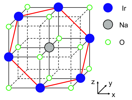
Figure 1: Crystal structure of Na₂IrO₃ in the cubic setting.

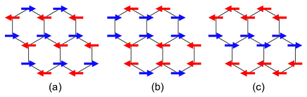
Figure 2: Possible magnetic orders in the honeycomb lattice; (a)the Néel order, (b)the stripy order, and (c)the zigzag order, respectively.

Several theoretical studies have already been carried out to explain those characteristics. The Kitaev-Heisenberg spin model Kitaev (2006); Chaloupka et al. (2010); Kimchi and You (2011); Chaloupka et al. (2013); Sizyuk et al. (2014) and a generic spin model Katukuri et al. (2014); Rau et al. (2014) have been derived by the strong coupling expansion based on the localized electron picture and the phase diagram has been examined in a wide range of parameter space. The zigzag alignment, unfortunately, seems to be realized only in rather extreme parameter values. Recently a spin model containing spin-spin anisotropic exchange couplings has been derived from the ab initio calculation, having led to the zigzag order in the ground state Yamaji et al. (2014). As for the itinerant electron picture, the band calculations based on the DFT have been carried out Mazin et al. (2012); Foyevtsova et al. (2013); Kim et al. (2014b). It is found that quasimolecular orbitals are formed within a hexagon of six Ir ions, resulting in the insulating ground state. Recently the self-interaction correction (SIC) has been done to the DFT Kim et al. (2014b), and makes the zigzag spin order stabilize in the ground state. Accordingly the itinerant electron picture may provide a good starting point.

When we turn our attention to the collective excitation, three characters of the intensity of the excitation spectrum are identified by the experiment Choi et al. (2012); Gretarsson et al. (2013a, b) :magnetic excitation for $\omega<40$ meV, excitonic excitation around $\omega\sim$ 450 meV, and contribution from the continuum part 600 meV $<\omega$. Note that the last contribution is regarded as the transfer between $j_{\textrm{eff}}=\frac{3}{2}$ and $\frac{1}{2}$ in the localized electron picture. Despite intensive theoretical effort, collective excitations of Na₂IrO₃ have not been studied yet on the itinerant electron picture. In this paper, we investigate the collective excitations with the weak-coupling theory based on the itinerant picture to address the excitation spectra. To this end, we utilize a rather simple tight-binding model instead of ab initio calculation to clarify the underlying mechanism of the low-energy excitations. Employing the Hartree-Fock approximation (HFA) to the tight-binding model, we first calculate the one-electron energy as well as the ground-state energy. Then, we evaluate the density-density correlation function within the RPA with the help of the two-particle Green’s function in order to investigate the excitation spectra.

We consider the electron transfer mediated through O $2p$ orbitals and the direct $d$-$d$ transfer between Ir ions. When the direct $d$-$d$ transfer is weak, nearly flat and doubly degenerate bands come out due to the formation of quasimolecular orbitals as pointed out in previous studies Mazin et al. (2012); Foyevtsova et al. (2013); Kim et al. (2014b). Since one hole occupies in the $t_{2g}$ states per Ir ion and two Ir atoms are contained in the unit cell of the honeycomb lattice, the uppermost band is fully empty, thereby resulting in the energy gap between the occupied and unoccupied energy bands. The Coulomb interaction and magnetic order have minor influence on the formation of the energy gap, and hence the system may be called a band insulator. The zigzag magnetic order is found the most stable when the direct $d$-$d$ transfer is weaker than a certain value. However, the energy differences between the zigzag spin state and others such as the stripy, the Néel states are as small as several meV’s per Ir ion. Then, we calculate the density-density correlation function within the RPA on the zigzag order in ground state. In our calculation, the collective excitations come out as bound states as well as quasi-bound states with modifying the individual excitations of the electron-hole pair creation. With an appropriate value of the direct $d$-$d$ transfer, we find several bound states with the excitation energy concentrated on $\omega<50$ meV, which may be assigned as magnetic excitations. Other several bound states emerge in the energy region between $\omega\sim 350$ meV and the bottom of the energy continuum, which may be assigned as excitonic excitations. These features of excitation spectra semi-quantitatively capture the characteristic of the observed results mentioned above.

With increasing magnitude of the direct $d$-$d$ transfer between Ir ions, the nearly flat bands get dispersive, but the system remains still insulating state even for the sizable direct transfer. Within the HFA, the most stable magnetic order is, however, changed from the zigzag order to the Néel order when the direct $d$-$d$ transfer exceeds a certain value. In such a situation when the direct $d$-$d$ transfer is substantial, within the RPA on the Néel order, we have the bound states in the density-density correlation function, which are distributed in rather wide range of energy. Since this behavior is quite different from the experiment, the large direct $d$-$d$ transfer is unfavourable in real materials. Actually a recent analysis of the tight-binding parameters by the ab initio calculation has claimed that the structural distortions of all types suppress the direct $d$-$d$ transfer Foyevtsova et al. (2013).

The present paper is organized as follows. In §II, we introduce a multi-orbital tight-binding model. In §III, the electronic structure is evaluated within the HFA. In §IV, we calculate the density-density correlation function within the RPA. The excitation spectra are evaluated at the special k spots. Section V is devoted to the concluding remarks.

II Model Hamiltonian

Similar to the case of Sr₂IrO₄, each Ir ion in Na₂IrO₃ resides around the centre of oxygen octahedra. Due to the crystal electric field of IrO₆, the energy level of the $e_{g}$ orbitals of Ir atom is about 2-3 eV higher than that of the $t_{2g}$ orbitals. We take account of only $t_{2g}$ orbitals, and ignore the small lift of degeneracy arising from the distortion of IrO₆ octahedra in a first step. Thereby, as a minimal model, the Hamiltonian of a multi-orbital Hubbard model is defined on a honeycomb lattice,

$$H=H_{\rm SO}+H_{\rm I}+H_{\rm kin},$$ (1)

with

$$H_{\rm SO} = \zeta_{\rm SO}\sum_{i}\sum_{nn^{\prime}\sigma\sigma^{\prime}}d_{in\sigma}^{\dagger}({\bf L})_{nn^{\prime}}\cdot({\bf S})_{\sigma\sigma^{\prime}}d_{in^{\prime}\sigma^{\prime}},$$ (2)

$$H_{\rm I} = U\sum_{i,n}n_{in\uparrow}n_{in\downarrow}$$

$$+ \sum_{i,n<n^{\prime}\sigma}[U^{\prime}n_{in\sigma}n_{in^{\prime}-\sigma}+(U^{\prime}-J)n_{in\sigma}n_{in^{\prime}\sigma}]$$

$$+ J\sum_{i,n\neq n^{\prime}}(d_{in\uparrow}^{\dagger}d_{in^{\prime}\downarrow}^{\dagger}d_{in\downarrow}d_{in^{\prime}\uparrow}+d_{in\uparrow}^{\dagger}d_{in\downarrow}^{\dagger}d_{in^{\prime}\downarrow}d_{in^{\prime}\uparrow}),$$

$$H_{\rm kin} = \sum_{\left\langle i,i^{\prime}\right\rangle}\sum_{n,n^{\prime}\sigma}[\hat{T}_{i,i^{\prime}}]_{n,n^{\prime}}d_{in\sigma}^{\dagger}d_{i^{\prime}n^{\prime}\sigma}+{\rm H.c.},$$ (4)

where $H_{\rm SO}$, $H_{\rm I}$, and $H_{\rm kin}$ are described by the annihilation ($d_{in\sigma}$) and creation ($d_{in\sigma}^{\dagger}$) operators of $5d$ electron with orbital $n$ ($=yz,zx,xy$) and spin $\sigma$ at the Ir site $i$. The $\langle i,i^{\prime}\rangle$ indicates the nearest neighbour sum, and $n_{in\sigma}\equiv d_{in\sigma}^{\dagger}d_{in\sigma}$.

The $H_{\rm SO}$ describes the SOI of $5d$ electrons where ${\bf L}$ and ${\bf S}$ denote the orbital and spin angular momentum operators, respectively. We use the value $\zeta_{\rm SO}=0.4$ eV in the following calculation. The $H_{\rm I}$ represents the Coulomb interaction between the $t_{2g}$ electrons. Parameters satisfy $U=U^{\prime}+2J$ Kanamori (1963). We use the values $U=1.4$ eV, and $J/U=0.15$ in the following calculation. These parameter values for Ir atom have been utilized also in Sr₂IrO₄ Igarashi and Nagao (2013b, a).

The $H_{\rm kin}$ stands for the kinetic energy described by the hopping matrix $\hat{T}_{i,i^{\prime}}$. For simplicity, only transfers between the nearest neighbour Ir ions are taken into account. There are three types of bond between the nearest neighbour Ir ions, and we call them as bond 1, 2, and 3 as illustrated in figure 3 (a). Then, two kinds of electron transfer may contribute to $\hat{T}_{i,i^{\prime}}$ between the adjacent Ir-Ir pair. The one is indirect transfer via oxygen $2p$-orbitals ($\hat{T}_{i,i^{\prime}}^{(pd)}$), and the other is direct transfer between the Ir $5d$ orbitals ($\hat{T}_{i,i^{\prime}}^{(dd)}$). The former could take place only between the different $5d$ orbitals. It may be expressed in a matrix form with the bases $n=yz$, $zx$, $xy$ in order:

$$\hat{T}_{i,i^{\prime}}^{(pd)}=\left(\begin{array}[]{ccc}0&0&-t_{p}\\ 0&0&0\\ -t_{p}&0&0\end{array}\right),\left(\begin{array}[]{ccc}0&0&0\\ 0&0&t_{p}\\ 0&t_{p}&0\end{array}\right),\left(\begin{array}[]{ccc}0&t_{p}&0\\ t_{p}&0&0\\ 0&0&0\end{array}\right),$$ (5)

for $\langle i,i^{\prime}\rangle$ belonging to bonds 1, 2, and 3, respectively. Here $t_{p}$ may be evaluated by

$$t_{p}=V_{pd\pi}^{2}/E_{pd},$$ (6)

where $V_{pd\pi}$($=V_{pd\sigma}/\sqrt{3}$) stands for the Slater-Koster mixing parameter Slater and Koster (1954) between the O $2p$ and Ir $5d$ orbitals, and $E_{pd}$ denotes the charge-transfer energy from Ir $5d$ orbitals to O $2p$ orbitals. According to Harrison’s procedure Har , $V_{pd\sigma}$ and $E_{pd}$ may be estimated as $-1.8$ eV and $3$ eV, respectively, and hence $t_{p}$ is estimated as $0.375$ eV. As regards the direct $d$-$d$ transfer, the matrix $\hat{T}_{i,i^{\prime}}^{(dd)}$ may be expressed by means of the conventional Slater-Koster parameters $V_{dd\sigma}$, $V_{dd\pi}$ ($=-2V_{dd\sigma}/3$), and $V_{dd\delta}$ ($=V_{dd\sigma}/6$). Notice that it has non-zero matrix elements between the same $5d$ orbitals as well as between the different $5d$ orbitals. With the help of Harrison’s procedure, $V_{dd\sigma}$ is estimated as $-0.51$ eV. Since there exist several complications in real crystals, these values of transfer are regarded as providing only order of magnitude.

III Electronic structure within the Hartree-Fock Approximation

Before going to the HFA, it is instructive to investigate the situation with no Coulomb interaction working. Without magnetic orders, we can define a unit cell containing Ir ions A and B shown in figure 3(a). The corresponding first Brillouin zone (BZ) is illustrated as a smaller hexagon in figure 3(b). The one-electron energy is evaluated by diagonalizing $H_{\rm kin}+H_{\rm SO}$ for momenta in the BZ.

Figure 4 shows the one-electron energy with momenta along symmetry lines. The origin of the energy is set at the top of the valence band. Each line is doubly degenerated. In the absence of the direct $d$-$d$ transfer, the dispersion is flat or nearly flat for $\zeta_{SO}=0$ or $\zeta_{SO}=0.4$ eV, respectively (left top or bottom panel of figure 4). It indicates the formation of molecular orbitals within the Ir hexagon. Since one hole exists per Ir site and two Ir ions are contained in a unit cell, the uppermost band should be empty, indicating a non-magnetic insulating ground state. Then, introduction of the direct $d$-$d$ transfer changes the situation. As shown in the right panels of figure 4, it makes the bands dispersive, but the system is narrowly insulating. This situation contrasts with that of Sr₂IrO₄, where the so-called “$j_{\rm eff}=1/2$” band, which is doubly degenerated when ignoring the Coulomb interaction, is half occupied, indicating that the system is a metal in the absence of the Coulomb interaction.

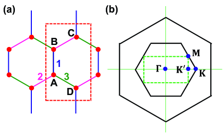
Figure 3: (a) Honeycomb lattice. Three types of bond represented by blue, magenta, and green lines are labeled as 1, 2, and 3, respectively. The unit cell consists of ions A and B. In the magnetic ordering phases, Ir atoms A, B, C, and D form a unit cell, which is enclosed by a broken line. (b)Reciprocal lattice and corresponding Brillouin zones. The hexagon attached by K and M forms the first Brillouin zone in the absence of magnetic orders, while the rectangle enclosed by a broken line forms the magnetic Brillouin zone. Centre and corners of larger hexagon represent the reciprocal lattice points.

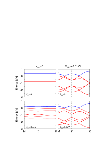
Figure 4: One-electron energy as a function of momenta along symmetry lines, when the Coulomb interaction is disregarded. The origin of energy is set at the top of the valence band. The conduction band is doubly degenerated. The left (right) panels show the results in the absence (presence) of direct $d$-$d$ transfer. The top (bottom) panels illustrate the results in the absence (presence) of the SOI.

Now we consider the situation that the Coulomb interaction turns on, and that a certain magnetic order such as the Néel, the stripy, or the zigzag orders, materializes in the ground state (see figure 2) Liu et al. (2011). To describe these orders, four sublattices A, B, C, and D, as shown in figure 3(a), are introduced. The corresponding first magnetic Brillouin zone (MBZ) is denoted as the rectangle enclosed by the broken line in figure 3(b). With wave vector ${\bf k}$ in the first MBZ, we define the Fourier transform of annihilation operator as

$$d_{\lambda n\sigma}({\bf k})=(4/N)^{\frac{1}{2}}\sum_{j}d_{jn\sigma}\textrm{e}^{-\\ textrm{i}{\bf k}\cdot{\bf r}_{j}},$$ (7)

where $j$ runs over the lattice sites belonging to one of the four sublattices A, B, C, and D specified by $\lambda$, and $N$ is the number of Ir ions.

With this notation, the one-electron energy $H_{0}\equiv H_{\rm kin}+H_{\rm SO}$ is rewritten as

$$H_{0}=\sum_{{\bf k}\xi\xi^{\prime}}d_{\xi}^{\dagger}({\bf k})\left[\hat{H}_{0}({\bf k})\right]_{\xi,\xi^{\prime}}d_{\xi^{\prime}}({\bf k}),$$ (8)

where use has been made of abbreviations $\xi=(\lambda,n,\sigma)$ and $\xi^{\prime}=(\lambda^{\prime},n^{\prime},\sigma^{\prime})$. The $[\hat{H}_{0}({\bf k})]_{\xi,\xi^{\prime}}$ denotes the matrix element of the Fourier transform of $H_{0}$ expressed in the $\xi$ basis.

We carry out the HFA by following the conventional procedure as explained in Igarashi and Nagao (2013b). First, we rewrite the Coulomb interaction as $H_{\rm I}$ $=$ $\frac{1}{2}\sum_{i}\sum_{\nu_{1},\nu_{2},\nu_{3},\nu_{4}}g(\nu_{1}\nu_{2};\nu_{3}\nu_{4})d_{i\nu_{1}}^{\dagger}d_{i\nu_{2}}^{\dagger}d_{i\nu_{4}}d_{i\nu_{3}}$ where $\nu_{m}\equiv(n_{m},\sigma_{m})$ with $m=$ 1, 2, 3, and 4. By comparing this with (LABEL:eq.H_Coulomb), we can determine the content of $g(\nu_{1}\nu_{2};\nu_{3}\nu_{4})$. Then, we replace $H_{\rm I}$ by

$$H_{\rm I}^{\rm HF}=\frac{1}{2}\sum_{j}\sum_{\xi_{1},\xi_{2},\xi_{3},\xi_{4}}\Gamma^{(0)}(\xi_{1}\xi_{2};\xi_{3}\xi_{4})\langle d_{j\xi_{2}}^{\dagger}d_{j\xi_{4}}\rangle d_{j\xi_{1}}^{\dagger}d_{j\xi_{3}},$$ (9)

with

$$\Gamma^{(0)}(\xi_{1}\xi_{2};\xi_{3}\xi_{4})=g(\xi_{1}\xi_{2};\xi_{3}\xi_{4})-g(\xi_{1}\xi_{2};\xi_{4}\xi_{3}),$$ (10)

where $\xi=(\lambda,\nu)$. The $\langle X\rangle$ denotes the ground-state average of operator $X$.

The expectation values of the electron density contained in $H_{\rm I}^{\rm HF}$ has to be self-consistently determined. For this purpose and evaluating the single-particle energy, it is convenient to introduce the single-particle Green’s function in a matrix form with $24\times 24$ dimensions,

$$\left[\hat{G}({\bf k},\omega)\right]_{\xi,\xi^{\prime}}=-\textrm{i}\int\langle T[d_{\xi}({\bf k},t)d_{\xi^{\prime}}^{\dagger}({\bf k},0)]\rangle{\rm e}^{\textrm{i}\omega t}{\rm d}t,$$ (11)

where $T$ is the time ordering operator, and $X(t)\equiv{\rm e}^{\textrm{i}H^{\prime}t}X{\rm e}^{-\textbf{i}H^{\prime}t}$ with $H^{\prime}=H_{0}+H_{\rm I}^{\rm HF}$. The Green’s function can be solved by diagonalizing the Hamiltonian matrix with $24\times 24$ dimensions. Let the $\ell$-th energy eigenvalue for ${\bf k}$ be $E_{\ell}({\bf k})$, and the corresponding wave function be $[\hat{U}({\bf k})]_{\xi,\ell}$. Then the Green’s function may be expressed as

$$[\hat{G}({\bf k},\omega)]_{\xi,\xi^{\prime}}=\sum_{\ell}\frac{[\hat{U}({\bf k})]_{\xi,\ell}[\hat{U}({\bf k})^{-1}]_{\ell,\xi^{\prime}}}{\omega-E_{\ell}({\bf k})\pm\textbf{i}\delta},$$ (12)

where $\delta$ denotes a positive convergent factor, and +(-) is taken when the energy level with $E_{\ell}({\bf k})$ is unoccupied (occupied). Note that

$$\langle d_{j\xi}^{\dagger}d_{j\xi^{\prime}}\rangle=\frac{4}{N}\sum_{{\bf k}}\int[-\textbf{i}\hat{G}({\bf k},\omega)]_{\xi,\xi^{\prime}}{\rm e}^{\textbf{i}\omega 0^{+}}\frac{{\rm d}\omega}{2\pi}.$$ (13)

Once we obtain the stable self-consistent solution, we could calculate the ground-state energy. Noting that

$$\sum_{{\bf k}\ell}E_{\ell}({\bf k})=\langle H_{0}\rangle+2\langle H_{\textrm{I}}^{\textrm{HF}}\rangle,$$ (14)

where the sum over $({\bf k}\ell)$ is restricted within the occupied levels, we express the ground-state energy as

$$\langle H^{\prime}\rangle=\frac{1}{2}\langle H_{0}\rangle+\frac{1}{2}\sum_{{\bf k}\ell}E_{\ell}({\bf k}).$$ (15)

Here $\langle H_{0}\rangle$ is evaluated by using (8) and (12):

$$\langle H_{0}\rangle=\sum_{{\bf k}\ell}\sum_{\xi\xi^{\prime}}[\hat{U}({\bf k})^{-1}]_{\ell,\xi^{\prime}}[H_{0}({\bf k})]_{\xi^{\prime},\xi}[\hat{U}({\bf k})]_{\xi,\ell},$$ (16)

where the sum over $({\bf k}\ell)$ is again restricted within the occupied levels.

III.1 Numerical calculation

Since the staggered magnetic moment is directing along the crystal $a$ axis Ye et al. (2012); Liu et al. (2011), we assume this is the direction of the staggered moment for the Néel, stripy, and zigzag orders in the self-consistent procedure. As already mentioned, the parameter values are set $\zeta_{SO}=0.4$ eV, $U=1.4$ eV, and $J/U=0.15$ in the following. As regards the transfer, we fix the strength of the indirect transfer by setting $V_{pd\sigma}=-1.84$ eV and $E_{pd}=3.01$ eV, or equivalently, $t_{p}=0.375$ eV. With evaluating (16), we carry out the sum over ${\bf k}$ by dividing the MBZ into $120\times 60$ meshes. To achieve the convergence, the iteration of $100\sim 500$ times is necessary for some cases.

For $|V_{dd\sigma}|<0.23$ eV, we find the zigzag order is the most stable one among the zigzag, Néel, and stripy orders, but the energy differences among those states are rather small. For $V_{dd\sigma}=-0.1$ eV, for instance, the energy of the zigzag order is $0.007$ eV per Ir ion lower than that of the Néel order and $0.011$ eV lower than the energy of stripy order. The the orbital and spin moments are found to be parallel to each other with $\langle L_{a}\rangle=\pm 0.265$ and $\langle S_{a}\rangle=\pm 0.085$, hence the magnetic moment $0.435\mu_{\textrm{B}}$. The latter value should be compared with the experimental value $0.22\mu_{\textrm{B}}$. Figure 5(a) shows $E_{\ell}({\bf k})$ as a function of ${\bf k}$ along symmetry lines in the zigzag order for $V_{dd\sigma}=-0.1$ eV. The dispersion curves experience weak dispersion, particularly for the uppermost valence band and the conduction band. The band gap opens with the size of $\sim 0.5-0.8$ eV. Note that it is similar to the one-electron energy shown in the left panels of figure 4. The latter comes out from the non-magnetic state with the Coulomb interaction disregarded, implying that the energy gap between the occupied and unoccupied states is originated not from the Coulomb interaction but from the formation of quasimolecular orbitals on Ir hexagons Mazin et al. (2012); Foyevtsova et al. (2013). This interpretation is different from the one based on the simple localized electron picture, which leads to the Kitaev-Heisenberg spin model in the strong coupling theory. Note that the small dispersions of the conduction band and the uppermost valence band and the sizable band gap are comparable with those of the ab-initio calculation (Figure 4 (b) in Kim et al. (2014b) for example).

For $|V_{dd\sigma}|>0.23$ eV, we find the Néel state is the most stable one. For, $V_{dd\sigma}=-0.51$ eV, which value may be estimated by the Harrison’s procedure, the orbital and spin moments are found parallel to each other with $\langle L_{a}\rangle=\pm 0.095$ and $\langle S_{a}\rangle=\pm 0.012$, and hence the magnetic moment is $0.119\mu_{\textrm{B}}$. Figure 5 (b) shows $E_{\ell}(\textbf{k})$ as a function of k for $V_{dd\sigma}=-0.51$ eV. The dispersion depends considerably on ${\bf k}$ with rather small energy gap. Since the zigzag order is confirmed in the real Na₂IrO₃, the small value of $|V_{dd\sigma}|$ is reasonable in this respect.

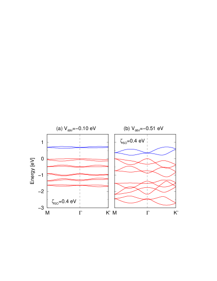
Figure 5: One-electron energy $E_{\ell}({\bf k})$ as a function of ${\bf k}$ along symmetry lines with (a) $V_{dd\sigma}=-0.1$ eV in the zigzag phase and (b) $V_{dd\sigma}=-0.51$ eV in the Neél phase. $U=1.4$ eV and $U^{\prime}/U=0.7$ with $2J+U^{\prime}=U$. Each band is doubly degenerated. The origin of energy is set at the top of the valence band.

IV Electron-hole pair excitations within the RPA

To investigate the elementary excitations, we consider the density-density correlation function defined by

$$\left[\hat{Y}^{+-}({\bf q},\omega)\right]_{\xi_{1}\xi^{\prime}_{1};\xi\xi^{\prime}}=\int_{-\infty}^{\infty}\langle[\rho_{{\bf q}\xi_{1}\xi^{\prime}_{1}}(t)]^{\dagger}\rho_{{\bf q}\xi\xi^{\prime}}(0)\rangle{\rm e}^{\textbf{i}\omega t}{\rm d}t,$$ (17)

with

$$\rho_{{\bf q}\xi\xi^{\prime}}=(4/N)^{\frac{1}{2}}\sum_{\bf k}d_{\xi}^{\dagger}({\bf k+q})d_{\xi^{\prime}}({\bf k}).$$ (18)

When ${\bf k+q}$ lies outside the first MBZ, it is reduced back to the first MBZ by a reciprocal vector ${\bf G}$. Since $\hat{Y}^{+-}({\bf q},\omega)$ is a matrix of $576\times 576$ dimensions, we consider a representative spectral function defined by

$$I({\bf q},\omega)\equiv\sum_{\xi\xi^{\prime}}\left[\hat{Y}^{+-}({\bf q},\omega)\right]_{\xi\xi^{\prime};\xi\xi^{\prime}}.$$ (19)

To evaluate the correlation function, we introduce the time-ordered Green’s function defined by

$$\left[\hat{Y}^{{\rm T}}({\bf q},\omega)\right]_{\xi_{1}\xi^{\prime}_{1};\xi\xi^{\prime}}=-\textbf{i}\int\left\langle T\left\{[\rho_{{\bf q}\xi_{1}\xi^{\prime}_{1}}(t)]^{\dagger}\rho_{{\bf q}\xi\xi^{\prime}}(0)\right\}\right\rangle{\rm e}^{\textbf{i}\omega t}{\rm d}t,$$ (20)

and use the fluctuation-dissipation theorem for $\omega>0$ Igarashi and Nagao (2013b),

$$\left[\hat{Y}^{+-}(q)\right]_{\xi_{1}\xi^{\prime}_{1};\xi\xi^{\prime}}=-\textbf{i}\left\{\left[\hat{Y}^{{\rm T}}(q)\right]^{*}_{\xi\xi^{\prime};\xi_{1}\xi^{\prime}_{1}}-\left[\hat{Y}^{{\rm T}}(q)\right]_{\xi_{1}\xi^{\prime}_{1};\xi\xi^{\prime}}\right\},$$ (21)

where $q\equiv({\bf q},\omega)$. The Green’s function $\hat{Y}^{+-}(q)$ can be evaluated by means of the particle-hole propagator. The derivation is concisely summarized below and the detail is given in Igarashi and Nagao (2013b).

We take account of the multiple scattering between particle-hole pair within the RPA. Then, the Green’s function is expressed as

$$\hat{Y}^{{\rm T}}(q)=\hat{F}(q)[\hat{I}+\hat{\Gamma}\hat{F}(q)]^{-1}=\left[\hat{F}(q)^{-1}+\hat{\Gamma}\right]^{-1},$$ (22)

where $\hat{I}$ is the unit matrix, and

$$[\hat{\Gamma}]_{\xi_{2}\xi^{\prime}_{2};\xi_{1}\xi^{\prime}_{1}}=\Gamma^{(0)}(\xi_{2}\xi^{\prime}_{1};\xi_{1}\xi^{\prime}_{2}).$$ (23)

Here the particle-hole propagator $\hat{F}(q)$ is defined as

$$[\hat{F}(q)]_{\xi_{2}\xi^{\prime}_{2};\xi_{1}\xi^{\prime}_{1}}$$

$$\equiv -\textbf{i}\frac{4}{N}\sum_{{\bf k}}\int\frac{{\rm d}k_{0}}{2\pi}[\hat{G}({\bf k+q},k_{0}+\omega)]_{\xi_{2}\xi_{1}}[\hat{G}({\bf k},k_{0})]_{\xi^{\prime}_{1}\xi^{\prime}_{2}}.$$

By substituting (12) into the single-particle Green’s function, and carrying out the integration over $k_{0}$ in (IV), we have

$$[\hat{F}(q)]_{\xi_{2}\xi^{\prime}_{2};\xi_{1}\xi^{\prime}_{1}} = \frac{4}{N}\sum_{{\bf k}}\sum_{\ell,\ell^{\prime}}U_{\xi_{2}\ell}({\bf k+q})U_{\xi_{1}\ell}^{*}({\bf k+q})U_{\xi^{\prime}_{1}\ell^{\prime}}({\bf k})U_{\xi^{\prime}_{2}\ell^{\prime}}^{*}({\bf k})$$ (25)

$$\times \left[\frac{[1-n_{\ell}({\bf k+q})]n_{\ell^{\prime}}({\bf k})}{\omega-E_{\ell}({\bf k+q})+E_{\ell^{\prime}}({\bf k})+\textbf{i}\delta}-\frac{n_{\ell}({\bf k+q})[1-n_{\ell^{\prime}}({\bf k})]}{\omega-E_{\ell}({\bf k+q})+E_{\ell^{\prime}}({\bf k})-\textbf{i}\delta}\right].$$

Equation (22) contains collective modes, which appear as bound states in the low-energy sector below the energy continuum of individual electron-hole pair excitations. Since $\hat{F}(q)$ is an Hermite matrix, $\hat{F}(q)^{-1}+\hat{\Gamma}$ can be diagonalized by a unitary matrix. If an eigenvalue becomes zero at $\omega=\omega_{\textrm{B}}({\bf q})$, $\omega_{\textrm{B}}({\bf q})$ is regarded as the bound-state energy. Let the corresponding eigenvector be $B_{\xi\xi^{\prime}}({\bf q})$. Then, expanding $[\hat{Y}^{{\rm T}}(q)]_{\xi_{1}\xi^{\prime}_{1};\xi\xi^{\prime}}$ around $\omega=\omega_{\textrm{B}}({\bf q})$, we have

$$\left[\hat{Y}^{{\rm T}}(q)\right]_{\xi_{1}\xi^{\prime}_{1};\xi\xi^{\prime}}=\frac{[\hat{C}({\bf q})]_{\xi_{1}\xi^{\prime}_{1};\xi\xi^{\prime}}}{\omega-\omega_{\textrm{B}}({\bf q})+\textbf{i}\delta},$$ (26)

with

$$[\hat{C}({\bf q})]_{\xi_{1}\xi^{\prime}_{1};\xi\xi^{\prime}}$$

$$= \frac{B_{\xi_{1}\xi^{\prime}_{1}}({\bf q})B_{\xi\xi^{\prime}}^{*}({\bf q})}{\sum_{\xi_{2}\xi^{\prime}_{2}\xi_{3}\xi^{\prime}_{3}}B_{\xi_{3}\xi^{\prime}_{3}}^{*}({\bf q})\frac{\partial[\hat{F}({\bf q},\omega_{\textrm{B}}({\bf q}))^{-1}]_{\xi_{3}\xi^{\prime}_{3};\xi_{2}\xi^{\prime}_{2}}}{\partial\omega}B_{\xi_{2}\xi^{\prime}_{2}}({\bf q})}.$$

Inserting (26) into the right hand side of (21), we have the correlation function,

$$\hat{Y}^{+-}(q)=2\pi\hat{C}({\bf q})\delta(\omega-\omega_{\textrm{B}}({\bf q})).$$ (28)

IV.1 Numerical calculation

We evaluate $\hat{F}(q)$ by summing over ${\bf k}$ in (25) with dividing the first MBZ into $40\times 30$ meshes. The bound states are determined by searching for $\omega$ to give zero eigenvalue in $\hat{F}(q)^{-1}+\hat{\Gamma}$ within the accuracy of 0.001 eV. The corresponding intensities are evaluated from finite difference between $\omega=\omega_{\textrm{B}}({\bf q})$ and $\omega=\omega_{\textrm{B}}({\bf q})+0.001$eV in (IV) in place of the differentiation. When $\omega$ enters into the energy continuum of individual electron-hole pair excitations, we need to evaluate the imaginary part arising from the denominator in (25). To make a rough estimate, we sort each $E_{\ell}({\bf k+q})-E_{\ell^{\prime}}({\bf k})$ inside the energy continuum in (25) into segments with the width of $0.05$ eV for $40\times 30$ ${\bf k}$-points, resulting in the histogram representation. Setting $\omega$ at the centre of each segment, we evaluate (25) and thereby (22).

For $|V_{dd\sigma}|<0.23$ eV, the zigzag order becomes the ground state as already mentionedCom (b). As a typical example in this region, we calculate the spectral function for $V_{dd\sigma}=-0.1$ eV. Top panel in figure 6 shows $I({\bf q},\omega)$ as a function of $\omega$ for ${\bf q}$ at $\Gamma$, $M$, and $K^{\prime}$ points. We have four bound states clustered in the region where $\omega$ is less than 50 meV for all the ${\bf q}$-points. They may be called as magnetic excitations ,which correspond to the hump A₀ in the RIXS spectra. Experimentally, INS detected a magnon mode below 6 meV Choi et al. (2012) while RIXS identified another around 35 meV Gretarsson et al. (2013b), which correspond well to our calculated results. The lowest excitation energy at the $\Gamma$ point is found around 9 meV. These magnetic excitations have quite a different origin from those of the Kitaev-Heisenberg spin model, since the former arise from the insulator based on the formation of quasimolecular orbitals on Ir hexagons, while the latter are brought about from the model based on the localized electron picture in the strong coupling theory. There are no spectral intensities in the region between $0.050$ eV$<\omega<0.340$ eV. In addition, we have found about a dozen of bound states in the region between $\omega=$0.340 eV and at the bottom of the energy continuum of individual electron-pair excitations, which may be called as the excitonic excitations and correspond to the RIXS spectra around the hump A. The continuous spectra start around $\omega=0.55-0.65$ eV, which may correspond to the RIXS spectra around the humps B and C. Accordingly, these capture qualitatively the characteristic of the RIXS spectra shown in the middle panel of figure 6.

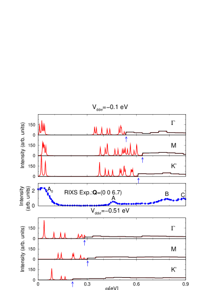
Figure 6: Spectral function $I({\bf q},\omega)$ as a function of $\omega$ for ${\bf q}$ at $\Gamma$, $M$, and $K^{\prime}$ points; the top panel for $V_{dd\sigma}=-0.1$ eV and the bottom panel for $V_{dd\sigma}=-0.51$ eV. The middle panel is the RIXS spectra taken from Gretarsson et al. (2013b) for ${\bf Q}=(0,0,6.7)$ in the $C2/m$ notation. The $\delta$-function peaks for bound states and the histograms for the continuum states are convoluted with the Lorentzian function of the half width half maximum 0.002 eV. The arrows indicate the lower boundary of the continuum spectra.

For $|V_{dd\sigma}|>0.23$ eV, the Néel state becomes the ground state. As a typical example in this region, we calculate the spectra for $V_{dd\sigma}=-0.51$ eV, which is shown in the bottom panel of figure 6. The bound states are distributed over a wide range of energy region below the continuum of electron-hole pair excitations. The number of the bound states are 9, 4, and 6 for ${\bf q}$ at $\Gamma$, $M$, and $K^{\prime}$ points, respectively. The magnetic and the excitonic excitations are not sharply separated. Such spectral distribution is quite different from the RIXS spectra shown on the middle panel in figure 6.

V Concluding remarks

We have studied excitation spectra in Na₂IrO₃ on the basis of the itinerant electron picture. We have employed a multi-orbital tight-binding model with the electron transfer mediated via the O $2p$ orbitals as well as the direct $d$-$d$ transfer, considering only the $t_{2g}$ orbitals for Ir ions on a honeycomb lattice. We have calculated the one-electron energy as well as the ground-state energy within the HFA, and then the density-density correlation function within the RPA. When the direct $d$-$d$ transfer is weak, it is found that the zigzag order becomes the ground state, and that the energy bands have small dispersions, probably due to the formation of quasimolecular orbitals. The energy differences between the zigzag order and other orders have been, however, as small as several meV per Ir ion. We have obtained the collective excitations as bound states in the density-density correlation function. Magnetic excitations have been concentrated in the energy region less than 50 meV, while excitonic excitations exist around $\omega>350$ meV, in qualitative agreement with the RIXS spectra. When the direct $d$-$d$ transfer has exceeded a certain value, on the other hand, the Néel order has become the ground state with the energy bands rather dispersive. The collective excitations have distributed over a wide range of excitation energy, which behavior is at variance with the RIXS spectra.

The $d$-$d$ transfer estimated by Harrison’s procedure is larger than the critical value. The above findings may indicate that, in Na₂IrO₃, the direct $d$-$d$ transfer is suppressed by the structural distortions of all types. This interpretation has been pointed out by a detailed analysis based on the ab initio band calculation Foyevtsova et al. (2013). Our present result lends support to this understanding from the point of view of the excitation spectra. To address this issue in more quantitative way, it may be necessary to calculate the excitation spectra in more realistic models. Finally electron correlations beyond the HFA and RPA may have important effects on the excitation spectra. Studies along these directions are left in future.