Persistent chimera states in nonlocally coupled phase oscillators

Abstract

Chimera states in the systems of nonlocally coupled phase oscillators are considered stable in the continuous limit of spatially distributed oscillators. However, it is reported that in the numerical simulations without taking such limit, chimera states are chaotic transient and finally collapse into the completely synchronous solution. In this Rapid Communication, we numerically study chimera states by using the coupling function different from the previous studies and obtain the result that chimera states can be stable even without taking the continuous limit, which we call the persistent chimera state.

The behavior of coupled oscillator systems can describe various pattern formations in a wide range of scientific fields Kuramoto (1984); Pikovsky et al. (2003). In the systems of nonlocally coupled identical oscillators, there often appears a strange phenomenon called the chimera state, which is characterized by the coexistence of coherent and incoherent domains, where the former domain consists of phase-locked oscillators and the latter domain consists of drifting oscillators with spatially changing frequencies Kuramoto and Battogtokh (2002); Abrams and Strogatz (2004); Shima and Kuramoto (2004); Abrams and Strogatz (2006); Abrams et al. (2008); Ott and Antonsen (2008, 2009); Martens et al. (2010); Omel’chenko et al. (2010); Wolfrum et al. (2011); Wolfrum and Omel’chenko (2011); Omelchenko et al. (2011, 2012); Tinsley et al. (2012); Hagerstrom et al. (2012); Omelchenko et al. (2013); Martens et al. (2013); Schmidt et al. (2014); Zhu et al. (2014); Haugland et al. (2015); Sethia et al. (2008); Maistrenko et al. (2014); Xie et al. (2014); Rosin et al. (2014). This interesting phenomenon was first discovered in the system of nonlocally coupled phase oscillators obeying the evolution equation

$$\frac{\partial}{\partial t}\theta(x,t)=\omega-\int dx^{\prime}G(x-x^{\prime})\,\Gamma(\theta(x,t)-\theta(x^{\prime},t))$$ (1)

with $2\pi$-periodic phases $\theta(x)$ on a finite interval $x\in[0,1]$ under the periodic boundary condition, a smooth $2\pi$-periodic coupling function $\Gamma$, and the kernel $G(y)=(\kappa/2)\exp(-\kappa|y|)$, where a constant $1/\kappa$ denotes the coupling range Kuramoto and Battogtokh (2002). Recently, similar spatiotemporal patterns have been found in various systems using, e.g., the logistic maps Omelchenko et al. (2011, 2012), Rössler systems Omelchenko et al. (2012), and FitzHugh-Nagumo oscillators Omelchenko et al. (2013).

In the study of the chimera state, the system, Eq. (1), with the sine coupling Sakaguchi and Kuramoto (1986)

$$\Gamma(\phi)=-\sin(\phi+\alpha)$$ (2)

is particularly important because of its simplicity and generality. In fact, this coupling function was used also in the first discovery of the chimera state Kuramoto and Battogtokh (2002). For numerical simulations, we usually discretize Eq. (1) into such a form as Eq. (3). In the simulations of such discretized systems, we can confirm that chimera states are surely stable in the continuous limit $N\rightarrow\infty$. However, the stability of chimera states in finitely discretized systems is questioned. In fact, it is reported that when $N$ is finite, chimera states with the sine coupling are chaotic transient and finally collapse into the completely synchronous solution Wolfrum et al. (2011); Wolfrum and Omel’chenko (2011); Rosin et al. (2014).

Recently, Ashwin and Burylko proposed the weak chimera similar to the chimera state, which is defined by the coexistence of frequency-synchronous and -asynchronous oscillators in the systems of coupled indistinguishable phase oscillators but is not necessarily spatially structured as coherent and incoherent domains Ashwin and Burylko (2015). They studied the weak chimera in some types of networks composed of the minimal number of oscillators with the Hansel-Mato-Meunier coupling, Eq. (4), and demonstrated that the weak chimera can be persistent (non transient). In this Rapid Communication, we study chimera states in the systems of nonlocally coupled phase oscillators with the Hansel-Mato-Meunier coupling by numerical simulation, and demonstrate that it is possible for persistent chimera states to appear.

As a model, we consider a ring of $N$ identical nonlocally coupled phase oscillators described as

$${\dot{\theta}}_{j}(t)=\omega+\frac{1}{2R}\sum^{j+R}_{k=j-R}\Gamma(\theta_{j}(t)-\theta_{k}(t))$$ (3)

with $2\pi$-periodic phases $\theta_{j}$ ($j=1,\ldots,N$). This model corresponds to a spatially discretized version of Eq. (1) with a constant kernel within a certain range. The natural frequency $\omega$ of the oscillators can be set to zero without loss of generality, and the nonlocal coupling range $R$ needs to satisfy $1<R<(N-1)/2$. In this Rapid Communication, we fix $R/N\sim 0.35$. As the coupling function $\Gamma(\phi)$, we choose the Hansel-Mato-Meunier coupling Hansel et al. (1993)

$$\Gamma(\phi)=-\sin(\phi+\alpha)+r\sin(2\phi),$$ (4)

where $\alpha$ is the phase lag parameter of the fundamental harmonic component and $r$ is the amplitude ratio of the second harmonic component. For $r=0$, Eq. (4) recovers the sine coupling, Eq. (2). In the systems of globally coupled phase oscillators, it is known that such higher harmonic components in the coupling function are responsible for a rich variety of synchronous patterns excluded by the sine coupling Hansel et al. (1993); Daido (1992); Okuda (1993); Daido (1996); Kori and Kuramoto (2001); Ashwin et al. (2008). Therefore we expect that also in the systems of nonlocally coupled phase oscillators with Eq. (4), we could observe new chimera patterns excluded by the sine coupling.

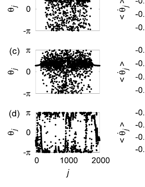
Figure 1: Results of numerical simulation of Eq. (3) with $N=2000$ and $\alpha=1.46$. In each row, the left panel shows the snapshot of phase $\theta_{j}$, and the right panel shows the profile of the average frequency $\langle\dot{\theta}_{j}\rangle$ with $T=5000$ and $t_{\text{rel}}=2000$ in Eq. (6). For (a) $r=0.001$, (b) $r=0.03$, and (c) $r=0.06$, chimera states are observed, while they are not observed for (d) $r=0.12$.

First, we consider the case of sufficiently large $N$ corresponding to the continuous limit. Figure 1 shows the results of numerical simulation of Eq. (3) with Eq. (4) for several $r\geq 0$. For all the simulations of the present Rapid Communication, we used the fourth-order Runge-Kutta method with time interval $\Delta t=0.01$. In Fig. 1, we fix $\alpha=1.46$, for which chimera states are observed in the case of the sine coupling ($r=0$). As initial conditions, we used

$$\theta_{j}(0)=6\exp\left[-30\left(\frac{j}{N}-\frac{1}{2}\right)^{2}\,\right]R_{j},$$ (5)

where $R_{j}\in[-1/2,1/2]$ is a uniform random number, which is so close to a chimera state as to assist its emergence Abrams and Strogatz (2006).

In our simulation, chimera states are observed for $r<0.073$ as shown in Figs. 1(a)-1(c). The phase pattern (left panels) is clearly separated into coherent and incoherent domains, which is characteristic of the chimera state. From the right panels of this figure, we can see that the average frequency

$$\langle\dot{\theta}_{j}\rangle(T)=\frac{1}{T}\int^{t_{\text{rel}}+T}_{t_{\text{rel}}}\dot{\theta}_{j}(t)\,dt$$ (6)

of each oscillator in the coherent domain is almost constant, where $T$ is the measurement time and $t_{\text{rel}}$ is the relaxation time, while the frequency in the incoherent domain varies continuously. For $r\geq 0.073$, chimera states gradually disappear as $r$ increases. In addition, for $r\geq 0.110$, chimera states are not observed, but each oscillator evolves almost independently, where the average frequency seems to converge to a constant value in the limit of $T\rightarrow\infty$, though the frequency in Fig. 1(d) still exhibits some fluctuations due to a finite $T$. The survey of these behaviors is depicted in Fig. 2.

Figure 2: Phase diagram of stable solutions to Eq. (3) with Eq. (4) at $\alpha=1.46$ in the continuous limit ($N=2000$). Horizontal lines denote the stability regions of each solution. We have not clearly determined the transition between the chimera state and almost independent oscillation yet. Note that the stability region of the wave solution with the wave number $k=1$ does not cover $r=0$.

From the linear stability analysis, it is found that the completely synchronous solution $\theta_{1}=\theta_{2}=\cdots=\theta_{N}$ to Eq. (3) with Eq. (4) is stable for $r<(\cos\alpha)/2$ ($\simeq 0.055$ at $\alpha=1.46$). Moreover, chimera states also appear to be stable in this parameter region [see Figs. 1(a) and 1(b)]. However, it is reported that when $N$ is finite, chimera states at $r=0$ are transient and finally collapse into the completely synchronous state Wolfrum and Omel’chenko (2011). We below confirm whether these chimera states, particularly for $r>0$, are transient or really stable even when $N$ is finite.

Figure 3: Average lifetime $\tau$ of the chimera state as varying $r$ at the parameters $N=30$ and $\alpha=1.46$. A point in the figure is the average over $1000$ simulations from different initial conditions obeying Eq. (5).

Figure 4: Log-log plot of the data $(\Delta r,\tau)$ for $r^{\ast}=0.035$ (diamond), $0.039$ (circle), $0.045$ (cross), $0.050$ (square) and $0.055$ (triangle). The data for $r^{\ast}=0.039$ are fitted linearly by the least squares method (black line), where we used only the data $\tau\geq 300000$ to obtain better linearity for this fitting.

Figure 4 shows the average lifetime $\tau$ of the chimera state for $N=30$, as increasing $r$ from $0$ to $(\cos\alpha)/2\simeq 0.055$. Here we regard the lifetime of the chimera state as the time at which the completely synchronous state appears, i.e., the global order parameter

$$Z(t)=\left|\frac{1}{N}\sum_{k=1}^{N}e^{i\,\theta_{k}}\right|$$ (7)

reaches $Z(t)=1$. As for the chimera state in the finite $N$ cases, it should be noted that it is difficult to judge the emergence of the chimera state, because the spatial position of the chimera state does not stay still but fluctuates Omel’chenko et al. (2010), in particular, more violently as $N$ becomes smaller. In fact, in the case of $N=30$, we could not observe the characteristic profile of the average frequency as in the right panels of Figs. 1(a)-1(c). However, we observed that the coherent domain exists in the phase snapshots as in the left panels of Figs. 1(a)-1(c), which convinces us of the emergence of the chimera state.

For Fig. 4, it should be noted that there is a possibility that chimera states collapse into a stable solution other than the completely synchronous state. From the linear stability analysis, we can show that the wave solution $\theta_{i}=\theta_{1}+2\pi k(i-1)/N$ Sethia et al. (2008); Xie et al. (2014) with the wave number $k=1$ is also stable for $r\geq 0.003$ (Fig. 2). This implies that chimera states may collapse into the wave solution. However, we never observed such collapse in our simulations from $1000$ different initial conditions, Eq. (5), at each $r$.

As $r$ is increased, the average lifetime $\tau$ increases monotonically, and appears to diverge to infinity at a certain $r=r^{\ast}$. Assuming some values as $r^{\ast}$, we obtain Fig. 4 by the log-log plot of the data $(\Delta r,\tau)$, where $\Delta r\equiv r^{\ast}-r$. From this figure, we can assume the power law

$$\tau\propto(\Delta r)^{-\zeta}$$ (8)

and we determine $r^{\ast}\simeq 0.039$ from the best linear fitting of the data. Since $r^{\ast}<(\cos\alpha)/2\simeq 0.055$, this implies that there exists a parameter region where the chimera state (with infinite lifetime) and the completely synchronous state are bistable even in the finite $N$ cases. However, we cannot exclude the possibility of $r^{\ast}=(\cos\alpha)/2$, because it is difficult to obtain the exact value of $r^{\ast}$ due to divergent simulation time.

Next, we investigate the chimera state of $N=30$ for $r>(\cos\alpha)/2$, where the completely synchronous state is unstable. The possibility that chimera states appear in the region without the stable completely synchronous state differs from the case of the sine coupling. In this region, chimera states cannot collapse into the completely synchronous state. Though the wave solution with $k=1$ is stable in this region, we never observed that chimera states collapse into the wave solution within our maximum simulation time $t=2\times 10^{8}$. Therefore, the collapse of the chimera state should not occur if other stable non-chimera solutions do not exist. Though we searched for stable non-chimera solutions other than the wave solution by extensive numerical simulations, we could not find any such solutions. From the above results, we conclude that, in a certain range of $r>(\cos\alpha)/2$, the chimera state and the wave solution are bistable, and the chimera state can be persistent (non-transient) even in the finite $N$ cases. This result is consistent with $\tau\rightarrow\infty$ for $r>r^{\ast}$, as seen in Fig. 4.

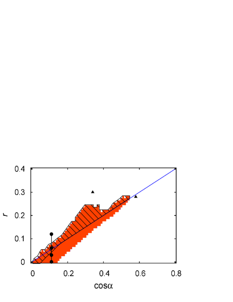
Figure 5: (Color online) Stability region of the chimera state (red) on the $(\cos\alpha,r)$ plane in the continuous limit ($N=2000$). The hatched region corresponds to the persistent chimera state, that is, the stability region of the chimera state in the case of $N=30$. The blue line denotes $r=(\cos\alpha)/2$, and the completely synchronous solution is stable for $r<(\cos\alpha)/2$. Black circles denote the parameter values of Fig. 1. Black triangles denote the parameter values of Fig. 7, where multichimera states appear.

Investigating the chimera states in the $(\cos\alpha,r)$ parameter space, we obtained Fig. 5. The red region corresponding to the chimera state in the continuous limit ($N=2000$) is spread around $r=(\cos\alpha)/2$. In the finite $N$ cases, the chimera state for small $r$ becomes transient, while the chimera state for large $r$ remains persistent, as seen at least for $r>(\cos\alpha)/2$ of the red region. For $\cos\alpha<0.15$, we can see that there exists a region $r^{\ast}<r<(\cos\alpha)/2$ where the chimera state is persistent in the case of $N=30$. Note that the stability region of the persistent chimera state (hatched in Fig. 5) extends to the $r=0$ line, which implies that the chimera state with the sine coupling can be persistent (non-transient) even in the finite $N$ cases. Specifically, the average lifetime $\tau$ of the chimera state increases similarly to Fig. 4 as $\cos\alpha$ is decreased on the $r=0$ line, and diverge at $\cos\alpha^{\ast}\simeq 0.044$. However, this fact does not contradict the previous study that shows the transient chimera state Wolfrum and Omel’chenko (2011), because the parameter $\alpha$ in that study corresponds to the line of black circles in Fig. 5, which has a larger $\cos\alpha$ than our hatched region on the $r=0$ line.

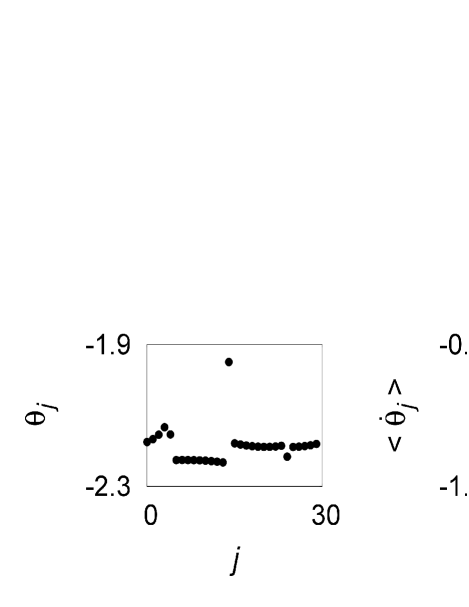
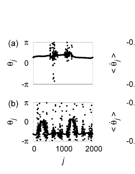
Figure 6: Weak chimera for Eq. (3) with $N=30$, $\alpha=1.46$, and $r=0.032$, which are the parameter values on the line of black circles in Fig. 5. The snapshot of phase $\theta_{j}$ (left) and the profile of the average frequency $\langle\dot{\theta}_{j}\rangle$ (right).

Figure 7: Multichimera states for Eq. (3) with $N=2000$. The left panels show the snapshot of phase $\theta_{j}$, and the right panels show the profile of the average frequency $\langle\dot{\theta}_{j}\rangle$ with $T=5000$ and $t_{\text{rel}}=2000$ in Eq. (6). Parameter values are (a) $\alpha=0.95$ and $r=0.28$, and (b) $\alpha=1.22$ and $r=0.30$, which are plotted in Fig. 5.

In summary, we studied chimera states in the systems of nonlocally coupled phase oscillators, Eq. (3), with the Hansel-Mato-Meunier coupling, Eq. (4), by numerical simulations, motivated by the result that chimera states with the sine coupling, Eq. (2), in finitely discretized systems are chaotic transient and finally collapse into the completely synchronous state Wolfrum and Omel’chenko (2011). The existence of chimera states was examined in the parameter space ($\alpha,r$) in Eq. (4), and the chimera states were observed around $r=(\cos\alpha)/2$ in the continuous limit $N\rightarrow\infty$. For $r<(\cos\alpha)/2$, the chimera state and the completely synchronous state can be bistable. In this region of the finite $N$ cases, the chimera state is transient for $r<r^{\ast}$, but it is persistent for $r^{\ast}<r<(\cos\alpha)/2$. Moreover, even for $r>(\cos\alpha)/2$, it is persistent in the region where the chimera state in $N\rightarrow\infty$ is stable. At first, we expected the chimera state to become persistent due to the destabilization of the completely synchronous state by the effect of $r$, but have obtained the persistent chimera state not only in the unstable region of the completely synchronous state as expected but also in its stable region. As a result, we have discovered that the chimera state in the case of the sine coupling can also be persistent by using appropriate $\alpha$ in the stability region of the completely synchronous state. Though we have numerically found the persistent chimera state in this Rapid Communication, its bifurcation-theoretical understanding is still an open problem.

When we investigated the collapse of chimera states at $\alpha=1.46$, we infrequently observed that a chimera state collapses into a weak chimera characterized by the coexistence of frequency-synchronous and -asynchronous oscillators Ashwin and Burylko (2015); Bick and Ashwin (2015), as shown in Fig. 7. In Ashwin and Burylko (2015), the existence of weak chimeras for Eq. (3) with Eq. (4) is confirmed in the system with a small number of oscillators ($N=4$, $6$, and $10$). In our numerical simulation with a larger number of oscillators ($N=30$), such a weak chimera is stable in a small range of $r<(\cos\alpha)/2$, for example, $0.032\leq r\leq 0.040$ at $\alpha=1.46$.

Moreover, as other solutions, we observed multichimera states, which have two or more incoherent domains Omelchenko et al. (2013); Sethia et al. (2008); Maistrenko et al. (2014); Xie et al. (2014), for Eq. (3) with Eq. (4) in the continuous limit ($N=2000$), as shown in Fig. 7. Other than the black triangles in Fig. 5, we observed multichimera states in a large region of the parameter space, though we do not describe the region in detail because it is beyond the scope of the present Rapid Communication.

References

- Kuramoto (1984) Y. Kuramoto, Chemical Oscillation, Waves, and Turbulence (Springer, Berlin, 1984).
- Pikovsky et al. (2003) A. Pikovsky, M. Rosenblum, and J. Kurths, Synchronization: A Universal Concept in Nonlinear Sciences (Cambridge University Press, Cambridge, 2003).
- Kuramoto and Battogtokh (2002) Y. Kuramoto and D. Battogtokh, Nonlinear Phenom. Complex Syst. 5, 380 (2002).
- Abrams and Strogatz (2004) D. M. Abrams and S. H. Strogatz, Phys. Rev. Lett. 93, 174102 (2004).
- Shima and Kuramoto (2004) S. I. Shima and Y. Kuramoto, Phys. Rev. E 69, 036213 (2004).
- Abrams and Strogatz (2006) D. M. Abrams and S. H. Strogatz, Int. J. Bifurcation Chaos 16, 21 (2006).
- Abrams et al. (2008) D. M. Abrams, R. Mirollo, S. H. Strogatz, and D. A. Wiley, Phys. Rev. Lett. 101, 084103 (2008).
- Ott and Antonsen (2008) E. Ott and T. M. Antonsen, Chaos 18, 037113 (2008).
- Ott and Antonsen (2009) E. Ott and T. M. Antonsen, Chaos 19, 023117 (2009).
- Martens et al. (2010) E. A. Martens, C. R. Laing, and S. H. Strogatz, Phys. Rev. Lett. 104, 044101 (2010).
- Omel’chenko et al. (2010) O. E. Omel’chenko, M. Wolfrum, and Y. L. Maistrenko, Phys. Rev. E 81, 065201(R) (2010).
- Wolfrum et al. (2011) M. Wolfrum, O. E. Omel’chenko, S. Yanchuk, and Y. L. Maistrenko, Chaos 21, 013112 (2011).
- Wolfrum and Omel’chenko (2011) M. Wolfrum and O. E. Omel’chenko, Phys. Rev. E 84, 015201(R) (2011).
- Omelchenko et al. (2011) I. Omelchenko, Y. Maistrenko, P. Hövel, and E. Schöll, Phys. Rev. Lett. 106, 234102 (2011).
- Omelchenko et al. (2012) I. Omelchenko, B. Riemenschneider, P. Hövel, Y. Maistrenko, and E. Schöll, Phys. Rev. E 85, 026212 (2012).
- Tinsley et al. (2012) M. R. Tinsley, S. Nkomo, and K. Showalter, Nat. Phys. 8, 662 (2012).
- Hagerstrom et al. (2012) A. M. Hagerstrom, T. E. Murphy, R. Roy, P. Hövel, I. Omelchenko, and E. Schöll, Nature Phys. 8, 658 (2012).
- Omelchenko et al. (2013) I. Omelchenko, O. E. Omel’chenko, P. Hövel, and E. Schöll, Phys. Rev. Lett. 110, 224101 (2013).
- Martens et al. (2013) E. A. Martens, S. Thutupalli, A. Fourriére, and O. Hallatschek, Proc. Natl. Acad. Sci. U.S.A. 110, 10563 (2013).
- Schmidt et al. (2014) L. Schmidt, K. Schönleber, K. Krischer, and V. García-Morales, Chaos 24, 013102 (2014).
- Zhu et al. (2014) Y. Zhu, Z. Zheng, and J. Yang, Phys. Rev. E 89, 022914 (2014).
- Haugland et al. (2015) S. W. Haugland, L. Schmidt, and K. Krischer, Sci. Rep. 5, 9883 (2015).
- Sethia et al. (2008) G. C. Sethia, A. Sen, and F. M. Atay, Phys. Rev. Lett. 100, 144102 (2008).
- Maistrenko et al. (2014) Y. L. Maistrenko, A. Vasylenko, O. Sudakov, R. Levchenko, and V. L. Maistrenko, Int. J. Bifurcation Chaos 24, 1440014 (2014).
- Xie et al. (2014) J. Xie, E. Knobloch, and H.-C. Kao, Phys. Rev. E 90, 022919 (2014).
- Rosin et al. (2014) D. P. Rosin, D. Rontani, N. D. Haynes, E. Schöll, and D. J. Gauthier, Phys. Rev. E 90, 030902(R) (2014).
- Sakaguchi and Kuramoto (1986) H. Sakaguchi and Y. Kuramoto, Prog. Theor. Phys. 76, 576 (1986).
- Ashwin and Burylko (2015) P. Ashwin and O. Burylko, Chaos 25, 013106 (2015).
- Hansel et al. (1993) D. Hansel, G. Mato, and C. Meunier, Phys. Rev. E 48, 3470 (1993).
- Daido (1992) H. Daido, Prog. Theor. Phys. 88, 1213 (1992).
- Okuda (1993) K. Okuda, Physica D 63, 424 (1993).
- Daido (1996) H. Daido, Physica D 91, 24 (1996).
- Kori and Kuramoto (2001) H. Kori and Y. Kuramoto, Phys. Rev. E 63, 046214 (2001).
- Ashwin et al. (2008) P. Ashwin, O. Burylko, and Y. Maistrenko, Physica D 237, 454–466 (2008).
- Bick and Ashwin (2015) C. Bick and P. Ashwin, arXiv:1509.08824 (2015).