G-factors of hole bound states in spherically symmetric potentials in cubic semiconductors

Abstract

Holes in cubic semiconductors have effective spin 3/2 and very strong spin orbit interaction. Due to these factors properties of hole bound states are highly unusual. We consider a single hole bound by a spherically symmetric potential, this can be an acceptor or a spherically symmetric quantum dot. Linear response to an external magnetic field is characterized by the bound state Lande g-factor. We calculate analytically g-factors of all bound states.

I Introduction

Holes in cubic semiconductors originate from atomic p-orbitals. Therefore, the total angular momentum of a hole can take values $j=3/2$ and $j=1/2$. So the spin orbit split valence band consists of $j=3/2$ and $j=1/2$ subbands. In semiconductors with large fine structure the $j=1/2$ state is very high in energy and therefore is irrelevant. This is the case we consider here. Following tradition in the field, below we call the angular momentum of the hole “the effective spin” and denote it by letter $S$, $j\to S=3/2$. Studies of holes in cubic semiconductors have a long history. Pioneering theoretical work belongs to Luttinger who has applied the $k\cdot p$ method and the group theory analysis for hole quantum states near bottom of the band at the $\Gamma$ point luttinger . Quadratic in momentum Luttinger Hamiltonian depends on Luttinger parameters. The Hamiltonian has a rotationally invariant part which is independent of the lattice orientation and it also contains a small correction which is related to the cubic lattice and which is not rotationally invariant. In the present work we neglect the small rotationally noninvariant correction and consider the rotationally invariant Hamiltonian.

The hole binding in an acceptor level or in a quantum dot is a problem of a tremendous experimental interest. Theoretically shallow acceptor levels have been studied thoroughly, from the spherical approximation baldereschi_sph to accounting the lattice corrections baldereschi_cube , spin orbit split valence band baldereshi_Si_Ge , and so-called central cell correction baldereshi_Si_Ge ; fiorentini ; drachenko . As the acceptor spectrum is quite sensitive to variations of Luttinger parameters, the experimental data have been used to determine the parameters Said . The hole spectrum of the spherically symmetric quantum dot with infinite walls has also been calculated xia .

Zeeman splitting of acceptor levels in an external magnetic field has been also studied theoretically. The most detailed numerical calculation includes the rotationally invariant approximation, cubic lattice correction, and also higher order magnetic field corrections Schmitt . Results of this calculation have been used in analysis of numerous experimental data, see also malyshev . Experimental data on the shallow acceptor spectrum in magnetic field have been obtained predominantly from infrared absorption spectroscopy for different acceptors in GaAs atzmuller ; linnarsson ; lewis_gaas , Ge fisher ; baker ; vickers ; prakabar ; wang , Si ramdas ; kopf ; heijden and other semiconductors.

We already pointed out above that in the present work we disregard the spin-orbit split $j=1/2$-band and limit our analysis by the rotationally invariant approximation in the Luttinger Hamiltonian. This implies that our analysis is applicable for GaAs, InAs, InSb, and on the other hand the approximation is not justified in Si. We calculate analytically g-factors of hole bound states for acceptors and spherically symmetric single hole quantum dots. At corresponding values of parameters our results are consistent with that of previous numerical computations for acceptors Schmitt .

Structure of the paper is the following. In Section II we discuss the Hamiltonian and approximations. In Section III we calculate energy levels and wave functions of a hole bound by a spherically symmetric potential. This section is very similar to the paper baldereschi_sph . Nevertheless we present this section because of two reasons, (i) it introduces the method and the notations which we use in following sections. (ii) We calculate previously unknown energy levels in a spherical parabolic quantum dot. Section IV presents our main result, analytical calculation of Zeeman splitting. In Section V we specially consider the “ultrarelativistic” limit, the limit when mass of the heavy hole is diverging. Section VI presents tables of g-factors, and our conclusions are summarized in Section VII. Algebra of tensor operators is described in Appendix A, and the derivation of spin-orbit radial equations is given in Appendix B.

II Hamiltonian

Luttinger Hamiltonian for $S=3/2$ free hole in a zinc-blende semiconductor reads luttinger

$$H_{L}=\left(\gamma_{1}+\frac{5}{2}\gamma_{2}\right)\frac{{\bf p}^{2}}{2m}-\frac{\gamma_{2}}{m_{0}}\left(p_{x}^{2}S_{x}^{2}+p_{y}^{2}S_{y}^{2}+p_{z}^{2}S_{z}^{2}\right)$$

$$-\frac{\gamma_{3}}{m_{0}}\left(p_{x}p_{y}\{S_{x},S_{y}\}+p_{y}p_{z}\{S_{y},S_{z}\}+p_{z}p_{x}\{S_{z},S_{x}\}\right)\ ,$$

x, y, z are the crystal axes of the cubic lattice, ${\bf p}$ is the quasi-momentum, $m$ is the electron mass, $\gamma_{1}$, $\gamma_{2}$ and $\gamma_{3}$ are Luttinger parameters, and $\{...\}$ denotes the anticommutator. This Hamiltonian can be rewritten as

$$H_{L}=\left(\gamma_{1}+\frac{5}{2}\overline{\gamma}_{2}\right)\frac{{\bf p}^{2}}{2m}-\frac{\overline{\gamma}_{2}}{m}\left({\bf p}\cdot{\bf S}\right)^{2}+p_{i}p_{j}S_{m}S_{n}T^{(4)}_{ijmn}\ ,$$

where

$$\overline{\gamma}_{2}=\frac{2\gamma_{2}+3\gamma_{3}}{5}\ .$$

The irreducible 4th rank tensor $T^{(4)}_{ijmn}$ depends on the orientation of the cubic lattice, the tensor is proportional to $\gamma_{2}-\gamma_{3}$. Since in the large spin-orbit splitting materials $\gamma_{2}\approx\gamma_{3}$ the rotationally noninvariant part of the Hamiltonian can be neglected. Hence the Luttinger Hamiltonian can be approximated by the following rotationally invariant (independent of the lattice orientation) Hamiltonian

$$H_{L}\to H_{0} = \left(\gamma_{1}+\frac{5}{2}{\overline{\gamma}}_{2}\right)\frac{{\bf p}^{2}}{2m}-\frac{{\overline{\gamma}}_{2}}{m}\left({\bf p}\cdot{\bf S}\right)^{2}\ .$$ (1)

Since different components of momentum commute between themselves, $H_{0}$ can be rewritten as

$$H_{0} = \gamma_{1}\frac{{\bf p}^{2}}{2m}-\frac{{\overline{\gamma}}_{2}}{4m}Q_{ij}\tau_{ij}$$ (2)

$$\tau_{ij} = \left\{S_{i},S_{j}\right\}-\frac{2}{3}\delta_{ij}\cdot S(S+1)$$

$$Q_{ij} = \left\{p_{i},p_{j}\right\}-\frac{2}{3}\delta_{ij}\cdot p^{2}\ .$$

The $Q_{ij}\tau_{ij}$ term in (1) represents the effective spin orbit interaction. Therefore, it is convenient to introduce the parameter

$$\nu=\frac{2\overline{\gamma}_{2}}{\gamma_{1}}\ ,\ \ \ \nu<1\ ,$$

which characterizes the relative strength of the spin orbit interaction. Eigenstates of the Hamiltonian (1) have definite helicity, the projection of spin on the direction of momentum, $S_{p}=\pm 1/2$ (light holes) and $S_{p}=\pm 3/2$ (heavy holes). The corresponding masses are

$$m_{l}=\frac{m}{\gamma_{1}(1+\nu)}\ ,\ \ \ m_{h}=\frac{m}{\gamma_{1}(1-\nu)}\ .$$ (3)

In the limit $\nu\to 1$ mass of the heavy hole is diverging, $m_{h}\to\infty$, therefore we call this the “ultrarelativistic” limit, the limit corresponds to maximum possible spin orbit interaction.

To account for a magnetic field ${\bm{B}}$ imposed on the system one has (i) to account for the vector potential via the long derivative ${\bf p}\to\mbox{\boldmath{$\pi$}}={\bf p}-e{\bf A}$, and (ii) to account for the Zeeman contribution $\propto{\bf S}\cdot{\bf B}$. Here $e$ is the elementary electric charge. Since different components of $\pi$ do not commute there is a well known ambiguity between the gauge and the Zeeman terms. In particular, $(\mbox{\boldmath{$\pi$}}\cdot{\bf S})^{2}=\frac{1}{4}\{\pi_{i},\pi_{j}\}\cdot\{S_{i},S_{j}\}-\frac{e}{2}{\bf B}\cdot{\bf S}$. Therefore the Zeeman term added to Eq.(1) is different from that added to (2). Here we follow the standard convention Winkler to use $H_{0}$ from (2) with ${\bf p}\to\mbox{\boldmath{$\pi$}}={\bf p}-e{\bf A}$. In this case the spin Zeeman interaction is

$$H_{Z}=-2\kappa\mu_{B}{\bf B}\cdot{\bf S},$$ (4)

where $2\kappa\mu_{B}{\bf S}$ is the spin magnetic moment, $\mu_{B}$ is Bohr magneton, and value of $\kappa$ depends on the material Winkler . There is also cubic in spin Zeeman-like interaction

$$H_{Z}^{\prime}\propto S_{i}S_{j}S_{m}B_{n}T^{(4)}_{ijmn}\ ,$$ (5)

however it is small Winkler and we disregard it.

We restrict our analysis by linear in magnetic field approximation. Therefore, gauge terms, ${\bf p}\to\mbox{\boldmath{$\pi$}}={\bf p}-e{\bf A}$, also result in a magnetic moment. As usually, see Ref. Landau , we use the gauge ${\bf A}=[{\bf B}\times{\bf r}]/2$ to derive the orbital magnetic moment. All in all the operator of the total magnetic moment is $\mu_{B}{\bf\mathfrak{M}}$, where

$$\mathfrak{M}_{k}=2\kappa S_{k}+\gamma_{1}L_{k}-\gamma_{1}\frac{\nu}{4}T_{ijk}\tau_{ij}.$$ (6)

Here the first term corresponds to (4), the second term is the usual orbital magnetic moment which originates from the $\gamma_{1}$-term in Eq.(2), and the last term is a spin dependent magnetic orbital moment which originates from the $\gamma_{2}$-term in Eq.(2). The 3d-rank tensor in the last term is

$$T_{ijk}=\frac{1}{2}\left(\varepsilon_{ikn}\{x_{n},p_{j}\}+\varepsilon_{jkn}\{x_{n},p_{i}\}\right)\ ,$$ (7)

and $\tau_{ij}$ is defined in (2).

Thus, the total Hamiltonian which we consider in this work is

$$H=H_{0}+U(r)-\mu_{B}({\bf\mathfrak{M}}\cdot{\bf B})$$ (8)

where $U(r)$ is spherically symmetric potential attracting the hole.

III Energy levels and wave functions of a hole in a spherically symmetric potential

We already pointed out that this section is very similar to papers baldereschi_sph ; Schmitt . We present this section to introduce the method and the notations for further calculations of g-factors. Besides that we calculate previously unknown energy levels in a spherical quantum dot. The Hamiltonian (8) is invariant under rotations around the center of symmetry of the potential. Therefore, while because of the spin orbit interaction the orbital angular momentum ${\bf L}=[{\bf r}\times{\bf p}]$ is not conserved, the total angular momentum ${\bf J}={\bf L}+{\bf S}$ is conserved. The eigenstates of the Hamiltonian (8) are also the eigenstates of ${\bf J}^{2}=J(J+1)$ and $J_{z}=M$. The Hamiltonian contains only the orbital scalar ${\bf p}^{2}$ and the orbital quadrupole $Q_{ij}$. Therefore an eigenstate can be a combination of at most two values of orbital angular momentum with $\Delta L=2$, we denote by $L$ the minimum of these two values

$$\Psi(L,\!S,\!J,\!M)=f(r)\cdot|L,\!S,\!J,\!M\rangle+g(r)\cdot|L+2,\!S,\!J,\!M\rangle,$$ (9)

Radial wave functions are normalized $\int\limits_{0}^{\infty}dr\,r^{2}\left(|f|^{2}+|g|^{2}\right)=1.$ If $J\geq S=3/2$, only two values of $L$ are possible: $L=J-3/2$, $L=J-1/2$. The special case of $J=1/2$ realizes only at $L=1$ or $L=2$. In this case $g(r)\equiv 0$ and the wave function is

$$\Psi(L,S,J=1/2,M)=f(r)\cdot|L,S,J=1/2,M\rangle,$$ (10)

Interestingly, while the states with $J\geq S=3/2$ are constructed of both heavy and light holes, the states with $J=1/2$ are constructed of light holes only. Masses of light and heavy holes behave differently in the important limit $\nu\to 1$, see Eq.(3). We will see that this results in a qualitatively different behavior of $J\geq 3/2$ and $J=1/2$ energy levels and g-factors in the limit $\nu\to 1$.

To derive radial equations for functions $f$ and $g$ one has to use Wigner-Eckart theorem and algebra of spherical tensor operators. In Appendix A we remind the theorem and give definition of relevant spherical tensors. Equations for $f$ and $g$ are derived in Appendix B, here we just present the equations. For $J=1/2$ there is only one equation (we set $\hbar=1$)

$$\left[-\frac{1}{2m_{l}}\left(\partial_{rr}+\frac{2}{r}\partial_{r}-\frac{L(L+1)}{r^{2}}\right)+U(r)-E\right]f=0$$

(11)

We remind that here $L$ can only take values $L=1,2$. For $J\geq 3/2$ and $L=J-3/2$ the pair of coupled equations reads

$$\begin{array}[]{ll}\vspace{0.3 cm}\displaystyle\left[-\frac{\gamma_{1}}{2m}\left(1+\frac{\nu}{2}\frac{J-3/2}{J}\right)\right.&\left.\left(\displaystyle\partial_{rr}+\frac{2}{r}\partial_{r}-\displaystyle\frac{(J-1/2)(J-3/2)}{r^{2}}\right)+U(r)-E\right]f+\\ \vspace{0.3 cm}&+\displaystyle\frac{\nu\gamma_{1}}{4m}\frac{\sqrt{3(J-1/2)(J+3/2)}}{J}\left[\partial_{rr}+\frac{2(J+1)}{r}\partial_{r}+\frac{(J-1/2)(J+3/2)}{r^{2}}\right]g=0\end{array}$$ (14)

$$\begin{array}[]{ll}\vspace{0.3 cm}\displaystyle\left[-\frac{\gamma_{1}}{2m}\left(1-\frac{\nu}{2}\frac{J-3/2}{J}\right)\right.&\left.\left(\displaystyle\partial_{rr}+\frac{2}{r}\partial_{r}-\displaystyle\frac{(J+1/2)(J+3/2)}{r^{2}}\right)+U(r)-E\right]g+\\ &+\displaystyle\frac{\nu\gamma_{1}}{4m}\frac{\sqrt{3(J-1/2)(J+3/2)}}{J}\left[\partial_{rr}-\frac{2(J-1)}{r}\partial_{r}+\frac{(J+1/2)(J-3/2)}{r^{2}}\right]f=0\end{array}$$ (17)

Finally, for $J\geq 3/2$ and $L=J-1/2$ the pair of coupled equations is

$$\begin{array}[]{ll}\vspace{0.3 cm}\displaystyle\left[-\frac{\gamma_{1}}{2m}\left(1-\frac{\nu}{2}\frac{J+5/2}{J+1}\right)\right.&\left.\left(\displaystyle\partial_{rr}+\frac{2}{r}\partial_{r}-\displaystyle\frac{(J-1/2)(J+1/2)}{r^{2}}\right)+U(r)-E\right]f+\\ \vspace{0.3 cm}&+\displaystyle\frac{\nu\gamma_{1}}{4m}\frac{\sqrt{3(J-1/2)(J+3/2)}}{J+1}\left[\partial_{rr}+\frac{2(J+2)}{r}\partial_{r}+\frac{(J+1/2)(J+5/2)}{r^{2}}\right]g=0\end{array}$$ (20)

$$\begin{array}[]{ll}\vspace{0.3 cm}\displaystyle\left[-\frac{\gamma_{1}}{2m}\left(1+\frac{\nu}{2}\frac{J+5/2}{J+1}\right)\right.&\left.\left(\displaystyle\partial_{rr}+\frac{2}{r}\partial_{r}-\displaystyle\frac{(J+3/2)(J+5/2)}{r^{2}}\right)+U(r)-E\right]g+\\ &+\displaystyle\frac{\nu\gamma_{1}}{4m}\frac{\sqrt{3(J-1/2)(J+3/2)}}{J+1}\left[\partial_{rr}-\frac{2J}{r}\partial_{r}+\frac{(J-1/2)(J+3/2)}{r^{2}}\right]f=0\end{array}$$ (23)

Unlike Eq.(11) which contains only mass of the light hole, Eqs.(14) and (23) cannot be expressed solely in terms of the heavy hole mass. Both heavy and light holes contribute in $J\geq 3/2$ states. However, it is obvious that in the limit $\nu\to 1$, $m_{h}\to\infty$, the heavy hole dominates in the wave function and hence the energy must scale as

$$E\sim\frac{1}{m_{h}a^{2}},$$ (24)

where $a$ is the characteristic size of the wave function which also depends on $\nu$. Following Ref. baldereschi_sph we will use the standard spectroscopic notations for the quantum states, for example $1S_{3/2}$ indicates that $J=3/2$, the principal quantum number is $n=1$, and $L=0$ (of course there is also $L=2$ admixture).

Numerical integration of Eqs.(11),(14),(23) is straightforward. Here we consider two special cases, (i) parabolic potential, and (ii) Coulomb potential. The parabolic potential we take in the form

$$U(r)=\frac{(m/\gamma_{1})\omega^{2}r^{2}}{2}.$$

The ratio $E/\omega$ depends only on $\nu$. Plots of $E/\omega$ versus $\nu$ for several lowest states are presented in Fig.1. The ground state is $1S_{3/2}$. While energies of states with $J=1/2$ grow with $\nu$ approximately linearly, the energies of states with $J\geq 3/2$ scale as $E\propto\sqrt{1-\nu}$ in agreement with Eq.(24).

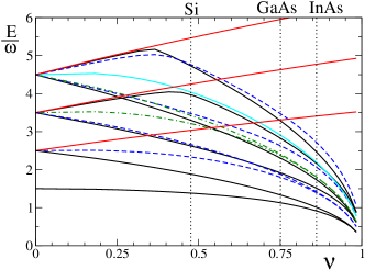
Figure 1: Energy levels versus $\nu$ in a parabolic quantum dot. The levels with $J=1/2$ are shown by solid red lines, $2P_{1/2}$, $3D_{1/2}$, $4P_{1/2}$ from bottom to top. The levels with $J=3/2$ are shown by solid black lines, $1S_{3/2}$, $2P_{3/2}$, $3S_{3/2}$, $4P_{3/2}$, $3D_{3/2}$, $4F_{3/2}$ from bottom to top. The levels with $J=5/2$ are shown by dashed blue lines, $2P_{5/2}$, $3D_{5/2}$, $4P_{5/2}$, $4F_{5/2}$ from bottom to top. The levels with $J=7/2$ are shown by dashed-dotted green lines, $3D_{7/2}$ and $4F_{7/2}$ from bottom to top. The level with $J=9/2$, $4F_{9/2}$ is shown by the solid cyan line. Vertical dotted lines indicate values of $\nu$ that correspond to particular compounds.

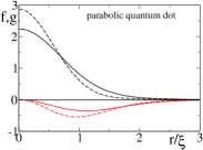
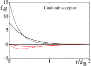
Figure 2: Radial wave functions of the ground state versus radius. Black lines show $f(r)$ and red lines show $g(r)$. Solid lines correspond to $GaAs$ and dashed lines correspond to $InAs$. The left panel correspond to the parabolic quantum well. The scale is $\xi=1/\sqrt{\omega m/\gamma_{1}}$. The right panel corresponds to the Coulomb acceptor. The scale is the effective Bohr radius, $a_{B}^{*}=[(m/\gamma_{1})(e^{2}/\epsilon)]^{-1}$.

For illustration we use Si, GaAs, and InAs. Values of Luttinger parameters from Ref.Winkler are presented in Table 1.

	$\gamma_{1}$	$\gamma_{2}$	$\gamma_{3}$	${\overline{\gamma}}_{2}$	$\nu$	$\kappa$
Si	4.285	0.339	1.446	1.00	0.47	-0.42
GaAs	6.85	2.1	2.9	2.58	0.75	1.2
InAs	20.4	8.3	9.1	8.78	0.86	7.6

Table 1: Luttinger parameters for Si, GaAs, and InAs.

Our approach is valid when $|\gamma_{2}-\gamma_{3}|$ is small compared to $\gamma_{2}$. Obviously, the approach is not valid in Si, on the other hand it is quite reasonable in GaAs and even better in InAs. Values of $\nu$ corresponding to Si, GaAs, InAs are shown in Fig.1 by vertical dotted lines. In the left panel of Fig.2 we plot radial wave functions of the quantum dot ground state for GaAs and InAs. The s-wave is dominating, the weight of the d-wave,

$$I_{1}=\int\limits_{0}^{\infty}dr\,r^{2}g^{2}$$ (25)

is 21% in GaAs and 32% in InAs.

Another example is attracting Coulomb center corresponding to acceptor impurity.

$$U(r)=-\frac{e^{2}/\epsilon}{r}\ ,$$

where $\epsilon$ is the dielectric constant. While this case has been thoroughly considered in the literature, we briefly present the results since we use them in the next Section. In this case the “atomic energy unit” is

$$E^{*}=(m/\gamma_{1})(e^{2}/\epsilon)^{2}\ .$$

The ratio $E/E^{*}$ is plotted in Fig.3 versus $\nu$ for several lowest states.

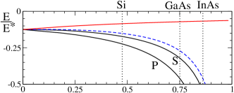
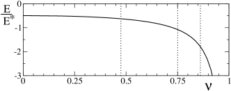
Figure 3: Coulomb acceptor energy levels versus $\nu$. The level with $J=1/2$, $2P_{1/2}$, is shown by the solid red line, top panel. The levels with $J=3/2$ are shown by solid black lines, $1S_{3/2}$, in the bottom panel and $2P_{3/2}$, $2S_{3/2}$, in the top panel. The level with $J=5/2$, $2P_{5/2}$, is shown by the dashed blue line, top panel. Note that the vertical axis scales are different in the top and in the bottom panels. Vertical dotted lines indicate values of $\nu$ that correspond to particular compounds.

In the right panel of Fig.2 we plot the acceptor ground state radial wave functions for GaAs and InAs. Again, the s-wave is dominating, the weight of the d-wave, $I_{1}$, is 26% in GaAs and 35% in InAs. Our results for the Coulomb acceptor are in excellent agreement with Ref. Schmitt .

IV Lande g-factor

The operator of magnetic moment $\mathfrak{M}$ is defined by Eq.(6). Hence Lande g-factor of a quantum state with given $J$ is defined by

$$\langle JM|\mathfrak{M}_{z}|JM\rangle=g\cdot M\ .$$

The operator $\mathfrak{M}$ contains a simple spin, $\propto{\bf S}$, and a simple orbital, $\propto{\bf L}$, contribution, as well as a more complex part dependent on the third rank tensor $T_{ijk}$, where the tensor is defined by (7). In order to apply the Wigner-Eckart formalism, we have to represent the third rank tensor in terms of irreducible tensors. It is easy to check that

$$T_{ijk}=\frac{1}{3}\left(\varepsilon_{nik}T^{(2)}_{jn}+\varepsilon_{njk}T^{(2)}_{in}\right)-$$

$$-\frac{1}{2}\left(\delta_{ik}L_{j}+\delta_{jk}L_{i}-2\delta_{ij}L_{k}\right),$$ (26)

where

$$T_{ij}^{(2)}=\frac{3}{4}\left(\{x_{i},p_{j}\}+\{x_{j},p_{i}\}\right)-\frac{1}{2}\delta_{ij}\{x_{n},p_{n}\}$$ (27)

is the irreducible tensor of the second rank. For the magnetic moment (6) we need only the convolution $T_{ijk}\tau_{ij}$. Therefore, we replace $T_{ijk}$ by the following simpler tensor which gives the same convolution.

$$T_{ijk}\to\tilde{T}_{ijk}=\frac{2}{3}\varepsilon_{njk}T^{(2)}_{in}-\delta_{jk}L_{i}.$$ (28)

Hence we can split the magnetic moment operator (6) into four parts $\mathfrak{M}_{z}=\mathfrak{M}_{S}+\mathfrak{M}_{1}+\mathfrak{M}_{2}+\mathfrak{M}_{3}$ which have different kinematic structures

$$\mathfrak{M}_{S}=2\kappa{\bf S}$$

$$\mathfrak{M}_{1}=\gamma_{1}{\bf L}$$

$$\mathfrak{M}_{2i}=\gamma_{1}\frac{\nu}{4}\tau_{ki}L_{k}$$

$$\mathfrak{M}_{3i}=-\gamma_{1}\frac{\nu}{6}\varepsilon_{nji}T_{kn}^{(2)}\tau_{kj}\ .$$ (29)

The Lande factor splits correspondingly

$$g=g_{s}+g_{1}+g_{2}+g_{3}$$

$$g_{s}=2\kappa\frac{\langle S_{z}\rangle}{M}$$

$$g_{1}=\gamma_{1}\frac{\langle L_{z}\rangle}{M}$$

$$g_{2}=\gamma_{1}\frac{\nu}{4}\frac{\langle\tau_{iz}L_{i}\rangle}{M}$$

$$g_{3}=-\gamma_{1}\frac{\nu}{6}\frac{\langle\varepsilon_{njz}T_{in}^{(2)}\tau_{ij}\rangle}{M}\ ,$$

where we average over the state $|JM\rangle$ given by Eq.(9) or Eq.(10).

IV.1 $\mathfrak{M}_{S}$ and $\mathfrak{M}_{1}$ contribution

The first two contributions, $g_{s}$ and $g_{1}$, in Eq.(IV) are usual textbook ones, they can be easily calculated via ordinary vector model Landau :

$$g_{s}\!=\!\kappa\!\left(1+\frac{S(S+1)-L(L+1)-4\left(L+\frac{3}{2}\right)I_{1}}{J(J+1)}\right)$$ (31)

$$g_{1}\!=\!\frac{\gamma_{1}}{2}\!\left(\!1+\!\frac{L(L+1)-S(S+1)+4\left(L+\frac{3}{2}\right)I_{1}}{J(J+1)}\right)$$ (32)

Here $I_{1}$, Eq.(25), is the weight of the component with higher orbital momentum $L+2$. Notice that $I_{1}=0$ for $J=1/2$.

IV.2 $\mathfrak{M}_{2}$ contribution

In Eqs.(IV),(IV) the operator $\mathfrak{M}_{2}$ is defined as product of Cartesian tensors, $\mathfrak{M}_{2i}\propto D_{i}=\tau_{ik}L_{k}$. On the other hand the tensor product theorem (70) is formulated in terms of spherical tensors where the product is defined in terms of Clebsch-Gordon coefficients $C^{\alpha\beta}_{\gamma\delta,\xi\zeta}$

$$D^{(1)}_{q}=\sum\limits_{q^{\prime}}C^{1q}_{1q^{\prime}2\,q-q^{\prime}}L^{(1)}_{q^{\prime}}\tau^{(2)}_{q-q^{\prime}}\ .$$ (33)

For $L_{i}$ and $\tau_{ij}$ we use the conventions (60), (61) to relate spherical and Cartesian components. Hence the relation between Cartesian and spherical components of $D$ is determined by (33).

$$D^{(1)}_{0}=C^{10}_{10,20}D_{z}=-\sqrt{\frac{2}{5}}D_{z}\ .$$

Now we can use the general tensor product formula (70) in combination with Wigner-Eckart theorem to find the matrix element of $D_{z}$

$$\langle L^{\prime},S,J,M|D_{z}|L,S,J,M\rangle=-M\sqrt{\frac{15}{2}\frac{2J+1}{J(J+1)}}\times$$

$$\ \ \ \times\left\{\begin{array}[]{ccc}1&2&1\\ L&S&J\\ L&S&J\end{array}\right\}\langle L||L^{(1)}||L\rangle\cdot\langle S||\tau^{(2)}||S\rangle\delta_{LL^{\prime}},$$ (37)

where $\{...\}$ is the $9j$-symbol and the reduced matrix elements are

$$\langle L||L^{(1)}||L\rangle = \sqrt{L(L+1)(2L+1)}$$

$$\langle S||\tau^{(2)}||S\rangle = \frac{1}{3}\sqrt{(2S-1)2S(2S+1)(2S+2)(2S+3)}$$ (38)

$$= 4\sqrt{5}\ .$$

In Eq.(37) we keep in mind that $f$ and $g$-components of the wave function differ by $\Delta L=2$, and the operator $D_{i}$ which is linear in $L$, does not connect these components. Hence, the $g_{2}$-Lande factor takes the form:

$$g_{2} =\gamma_{1}\frac{\nu}{4M}\langle\Psi|D_{z}|\Psi\rangle$$ (39)

$$=\gamma_{1}\frac{\nu}{4M}\left(\vphantom{\frac{1}{2}}\langle L,S,J,M|D_{z}|L,S,J,M\rangle\cdot(1-I_{1})+\right.$$

$$\ \ \ \ \left.\langle L+2,S,J,M|D_{z}|L+2,S,J,M\rangle\cdot I_{1}\right),$$

where the matrix elements are given by (37). Substituting $9j$-symbols we arrive to the following answer

$$J=1/2:$$

$$g_{2}=-\gamma_{1}\frac{5\nu}{3}\ \ \ if\ \ L=1$$

$$g_{2}=\gamma_{1}\nu\ \ \ \ \ \ \ if\ \ L=2$$

(40)

$$J\geq 3/2:$$

$$g_{2}=\gamma_{1}\frac{\nu}{2}\left(\frac{J-3/2}{J}-\frac{2J+1}{J+1}I_{1}\right)\ \ \ \ \ \ \ \ if\ L=J-3/2$$

$$g_{2}=\gamma_{1}\frac{\nu}{2}\left(\frac{J+5/2}{J+1}-\frac{2J+1}{J}(1-I_{1})\right)\ if\ L=J-1/2$$

IV.3 $\mathfrak{M}_{3}$ contribution

The calculation of the $\mathfrak{M}_{3}$ contribution is very similar to $\mathfrak{M}_{2}$. The operator $\mathfrak{M}_{3}$, Eqs.(IV),(IV), is defined as vector product of two irreducible Cartesian tensors $\tau$ and $T^{(2)}$ of second rank, $\mathfrak{M}_{3i}\propto R_{i}=\varepsilon_{nij}T^{(2)}_{kn}\tau_{kj}$. On the other hand the tensor product theorem (70) is formulated in terms of spherical tensors where the product is defined in terms of Clebsch-Gordon coefficients

$$R^{(1)}_{q}=\left(\tau^{(2)}\times T^{(2)}\right)_{1q}=\sum\limits_{q^{\prime}}C^{1q}_{2q^{\prime}2\,q-q^{\prime}}\tau^{(2)}_{q^{\prime}}T^{(2)}_{q-q^{\prime}}.$$ (41)

For $T^{(2)}_{ij}$ and $\tau_{ij}$ we use the convention (61) to relate spherical and Cartesian components. Hence the relation between Cartesian and spherical components of $R_{i}$ is determined by (41).

$$R_{0}^{(1)}=\frac{4i}{3}C^{10}_{2,-1;2,1}R_{z}=\frac{4i}{3\sqrt{10}}R_{z}.$$ (42)

According to (70), matrix elements of $R_{0}^{(1)}$ break into the product of reduced matrix elements for $T^{(2)}$ and $\tau$:

$$\langle L^{\prime},S,J,M|R^{(1)}_{0}|L,S,J,M\rangle=M\sqrt{\frac{3(2J+1)}{J(J+1)}}\times$$

$$\times\left\{\begin{array}[]{ccc}2&2&1\\ S&L^{\prime}&J\\ S&L&J\end{array}\right\}\langle L^{\prime}||T^{(2)}||L\rangle\cdot\langle S||\tau^{(2)}||S\rangle.$$ (46)

The reduced matrix element of $\tau^{(2)}$ is given in (IV.2). Non-zero reduced matrix elements for $T^{(2)}$ are

$$\langle L||T^{(2)}||L\rangle=-\sqrt{\frac{L(L+1)(2L+1)}{(2L-1)(2L+3)}}$$

$$\hskip 53.0pt\times\left(\vphantom{\frac{1}{2}}\{r,p_{r}\}-2i\right)$$

$$\langle L+2||T^{(2)}||L\rangle=\sqrt{\frac{3(L+1)(L+2)}{2(2L+3)}}$$ (47)

$$\hskip 70.0pt\times\left(\vphantom{\frac{1}{2}}\{r,p_{r}\}+i(2L+1)\right)$$

$$\langle L-2||T^{(2)}||L\rangle=\sqrt{\frac{3L(L-1)}{2(2L-1)}}$$

$$\hskip 70.0pt\times\left(\vphantom{\frac{1}{2}}\{r,p_{r}\}-i(2L+1)\right),$$

where $p_{r}=-i\partial_{r}$. The diagonal matrix element $\langle L||T^{(2)}||L\rangle$ gives zero after the r-integration, so there are no $ff$ and $gg$ terms in $\mathfrak{M}_{3}$. This is a direct consequence of the time reversal invariance, $T^{(2)}$ changes sign under time reversal and on the other hand it is impossible to construct a second rank tensor which is consistent with Wigner-Eckart and which changes sign under time reversal. This implies that $g_{3}$ is zero for $J=1/2$ states. However, the $fg$ contribution to $\mathfrak{M}_{3}$ which originate from (47) is nonzero. A direct calculation with (47) gives the following answer

$$g_{3}=i\gamma_{1}\sqrt{\frac{5}{2}}\cdot\frac{\nu}{4M}\cdot\langle\Psi|R^{(1)}_{0}|\Psi\rangle$$ (48)

$$\ \ \ =\gamma_{1}\nu\frac{\sqrt{3(J-1/2)(J+3/2)}}{2J(J+1)}\!\!\left[2\left(L+\frac{3}{2}\right)I_{2}+I_{3}\right]\ ,$$

where

$$I_{2}=\int\limits_{0}^{\infty}dr\,r^{2}f(r)g(r)$$

$$I_{3}=\int\limits_{0}^{\infty}dr\,r^{3}(fg^{\prime}-gf^{\prime})\ .$$ (49)

We remind our convention, $L$ is the minimum of two mixing orbital momenta, $L$ corresponds to $f$ and $L+2$ corresponds to $g$.

Eqs. (IV), (31), (32), (IV.2), and (48) solve the problem of g-factor of the hole bound state. Answers for $J=1/2$ states are universal

$$P_{1/2}:\ \ \ g=\frac{10}{3}\kappa-\frac{\gamma_{1}}{3}(2+5\nu)$$

$$D_{1/2}:\ \ \ g=-2\kappa+\gamma_{1}(2+\nu)\ .$$ (50)

Answers for $J\geq 3/2$ states are not universal, they depend on radial wave functions. In Section VI we present the results for parabolic quantum dot. However, before calculating numerical values of the g-factor we discuss the “ultrarelativistic” limit $\nu\to 1$.

V g-factor in “ultrarelativistic” $\nu\to 1$ limit

The case of maximum possible spin-orbit coupling $\nu\to 1$ ($\gamma_{1}=2\gamma_{2}$) is important as a theoretical limit and also some real materials such as InSb and InAs are pretty close to this limit. As it has been mentioned above, energies of $J\geq 3/2$ states in the limit $\nu\to 1$ satisfy the approximate relation (24). The states fall down on the bottom of the well. On the other hand, the states are described by equations (14) and (23). Because of collapse of the wave functions at $\nu=1$ we can neglect the energy and the potential in these Eqs. We keep only $\partial_{rr}$, $\frac{1}{r}\partial_{r}$ and $\frac{1}{r^{2}}$ terms. Excluding the second derivatives by subtraction of two coupled radial equations, we find the following relation between functions $f(r)$ and $g(r)$:

$$\alpha\left(f^{\prime}-\frac{L}{r}f\right)=g^{\prime}+\frac{L+3}{r}g$$ (51)

$$\alpha=\left\{\begin{array}[]{ccc}\sqrt{\frac{3(J-1/2)}{J+3/2}},\quad L=J-3/2,\\ \sqrt{\frac{J-1/2}{3(J+3/2)}},\quad L=J-1/2.\end{array}\right.$$ (54)

Multiplying Eq.(51) by $gr^{3}$ and separately by $fr^{3}$ and then integrating by parts keeping in mind the normalization condition, $\int f^{2}r^{2}dr=1-I_{1}$, one finds the following universal expression for the weight of the $g$-component in the “ultrarelativistic” limit

$$I_{1}=\left\{\begin{array}[]{ll}3(J-1/2)/(4J),&L=J-3/2,\\ (J-1/2)/(4(J+1)),&L=J-1/2.\end{array}\right.$$ (57)

The $g_{3}$-contribution (48) depends on the radial integrals $I_{2}$ and $I_{3}$ defined in Eq.(IV.3). The relation (51) is not sufficient to determine $I_{2}$ and $I_{3}$ separately. However, remarkably, the combination $2(L+3/2)I_{2}+I_{3}$ which enter Eq. (48) can be found from (51). Using the same derivation as (57) we find

$$2(L+3/2)I_{2}+I_{3}=-\frac{1}{2}\sqrt{3\left(J-\frac{1}{2}\right)\left(J+\frac{3}{2}\right)}\ .$$ (58)

Substitution of the integrals (57) and (58) in Eqs. (IV), (31), (32), (IV.2), and (48) gives the following values of the g-factors for $J\geq 3/2$

$$g_{s}=\frac{9\kappa}{2J(J+1)}$$

$$g_{1}=\gamma_{1}\left(1-\frac{9}{4J(J+1)}\right)$$

$$g_{2}=-\frac{\gamma_{1}}{4}\left(1+\frac{9}{4J(J+1)}\right)$$

$$g_{3}=-\frac{3\gamma_{1}}{4}\left(1-\frac{3}{4J(J+1)}\right)$$

$$g=\frac{9(2\kappa-\gamma_{1})}{4J(J+1)}\ .$$ (59)

Interestingly, Eqs.(V) are the same for $L=J-3/2$ and $L=J-1/2$. Thus in the “ultrarelativistic” limit, $\nu\to 1$, $g$-factors of $J\geq 3/2$ states depend only on $J$ and they are independent of a particular confinement (parabolic quantum dot, Coulomb acceptor,…) and independent of the radial quantum number. This universal behaviour is due to the collapse of heavy hole wave functions. Another point to note is the $\propto 1/[J(J+1)]$ dependence of the g-factor (V). This is similar to the g-factor dependence in diatomic molecules Landau . Physical reasons for this are also very similar, in the molecules the dependence is due to the spin-axis interaction, for holes the dependence is due to $\left({\bf p}\cdot{\bf S}\right)^{2}$ spin-momentum Luttinger interaction.

VI Numerical values of the Lande factor

We have already pointed out that, in principle, Eqs. (IV), (31), (32), (IV.2), (48) solve the problem of g-factor of the hole bound state. Still, to calculate numerical values of g-factors one needs to calculate integrals $I_{1}$, $I_{2}$, and $I_{3}$. The integrals immediately follow from wave functions found in Section III. We have checked that our results for g-factors of Coulomb acceptor states perfectly agree with that found numerically and tabulated in Ref. Schmitt . Below we present our results for three lowest states in parabolic quantum dot, $1S_{3/2}$, $2P_{3/2}$, $2P_{5/2}$, Tables 2, 3, and 4 respectively. We tabulate $g_{s}/\kappa$, $g_{1}/\gamma_{1}$, $g_{2}/\gamma_{1}$, $g_{3}/\gamma_{1}$ for different values of $\nu$. In the tables we also present separately the total orbital contribution $g_{L}$

$$g_{L}=g_{1}+g_{2}+g_{3},\quad g=g_{s}+g_{L}\ .$$

All lines in each table except of the lowest line are calculated with Eqs. (IV), (31), (32), (IV.2), (48) and with integrals $I_{1}$, $I_{2}$, $I_{3}$ calculated with functions $f$ and $g$ found numerically in Section III. The lowest lines are calculated directly with the “ultrarelativistic” Eqs.(V).

$\nu$	$g_{s}/\kappa$	$g_{1}/\gamma_{1}$	$g_{2}/\gamma_{1}$	$g_{3}/\gamma_{1}$	$g_{L}/\gamma_{1}$
0.6	1.83	0.087	-0.052	-0.285	-0.25
0.65	1.78	0.109	-0.071	-0.337	-0.299
0.7	1.73	0.135	-0.095	-0.392	-0.352
0.75	1.67	0.166	-0.125	-0.449	-0.408
0.8	1.59	0.203	-0.162	-0.505	-0.465
0.85	1.51	0.246	-0.209	-0.556	-0.519
0.9	1.408	0.296	-0.266	-0.596	-0.566
0.95	1.3	0.349	-0.332	-0.615	-0.597
1.0	1.2	0.4	-0.4	-0.592	-0.6

Table 2: g-factor contributions for $1S_{3/2}$ ground state in the parabolic quantum well at different values of $\nu$.

$\nu$	$g_{s}/\kappa$	$g_{1}/\gamma_{1}$	$g_{2}/\gamma_{1}$	$g_{3}/\gamma_{1}$	$g_{L}/\gamma_{1}$
0.6	1.375	0.312	-0.293	-0.251	-0.231
0.65	1.362	0.319	-0.313	-0.288	-0.282
0.7	1.347	0.326	-0.332	-0.327	-0.333
0.75	1.331	0.334	-0.349	-0.369	-0.384
0.8	1.314	0.343	-0.365	-0.412	-0.434
0.85	1.294	0.353	-0.380	-0.457	-0.484
0.9	1.271	0.365	-0.392	-0.504	-0.532
0.95	1.243	0.379	-0.400	-0.553	-0.574
1.0	1.2	0.4	-0.4	-0.592	-0.6

Table 3: g-factor contributions for the first excited $2P_{3/2}$ state in the parabolic quantum well at different values of $\nu$.

$\nu$	$g_{s}/\kappa$	$g_{1}/\gamma_{1}$	$g_{2}/\gamma_{1}$	$g_{3}/\gamma_{1}$	$g_{L}/\gamma_{1}$
0.6	0.897	0.552	-0.016	-0.427	0.108
0.65	0.841	0.579	-0.045	-0.483	0.052
0.7	0.784	0.608	-0.078	-0.534	-0.004
0.75	0.728	0.636	-0.116	-0.578	-0.058
0.8	0.674	0.663	-0.155	-0.615	-0.108
0.85	0.625	0.687	-0.197	-0.644	-0.153
0.9	0.582	0.709	-0.237	-0.665	-0.193
0.95	0.545	0.728	-0.277	-0.679	-0.228
1.0	0.514	0.743	-0.314	-0.677	-0.257

Table 4: g-factor contributions for the second excited $2P_{5/2}$ state in the parabolic quantum well at different values of $\nu$.

In all the cases there is a very strong compensation between spin, $g_{s}$, and orbital, $g_{L}$, contributions to the g-factor. For example, in GaAs ($\nu=0.75$), $g_{1S_{3/2}}=2.0-2.8=-0.8$, $g_{2P_{3/2}}=1.6-2.6=-1.0$, $g_{2P_{5/2}}=0.87-0.40=+0.47$. These compensations are somewhat similar to the compensation found in a particular situation in Ref. Uli . Here we see that the compensation is a generic effect related to the “ultrarelativistic” formula (V).

VII conclusions

We have developed analytical tensor theory of Lande g-factors in spherically symmetric bound states of holes in cubic semiconductors. The Lande factors are given by Eqs. (IV), (31), (32), (IV.2), (48) with integrals $I_{1}$, $I_{2}$, $I_{3}$ which depend on the quantum state wave function, see Eqs. (9), (25), (IV.3). We have shown that g-factors only weakly depend on the type of confinement (Coulomb acceptor, parabolic quantum dot, ….). Behaviour of g-factors in the “ultrarelativistic” limit is universal and completely independent of the type of confinement. This “ultrarelativistic” behaviour enforces a strong compensation between spin and orbital contributions to g-factors. It is worth noting that the developed tensor technique provides a solid basis for calculation of g-factor of asymmetric quantum dots, this problem will be addresses separately.

Acknowledgements We acknowledge Alex Hamilton, Tommy Li, Qingwen Wang, Ulrich Zuelicke and Roland Winkler for important discussions and interest to the work.

Appendix A irreducible tensors, Wigner-Eckart and tensor product theorems

In this Appendix we summarize the major equations from the SO(3) tensor algebra Landau which we use in our calculations. All tensors are defined in three-dimensional space. A tensor $R_{i_{1}i_{2}\dots i_{\ell}}$ of the rank $\ell$ is irreducible if its components can be transformed over some irreducible matrix representation $\mathfrak{D}_{\ell}$ of the rotational group SO(3). Consequently, the number of independent components of $R_{i_{1}i_{2}\dots i_{\ell}}$ coincides with the dimension of the representation $\dim\mathfrak{D}_{\ell}=2\ell+1$, whence we may choose the basis of these components $R_{m}^{(\ell)}$, $m=-\ell,\dots,\ell$ which have been transformed exactly like spherical harmonics $Y_{\ell m}$. This basis is usually called spherical basis. Spherical components of the vector ${\bf R}$ can be related to its Cartesian components in the following way

$$R_{0}^{(1)}=R_{z},\quad R_{\pm 1}^{(1)}=\mp\sqrt{\frac{1}{2}}(R_{x}\pm iR_{y})\ .$$ (60)

Similarly spherical harmonics of the second rank irreducible tensor $R^{(2)}$ can be related to its Cartesian components as

$$R_{0}^{(2)}=R_{zz},\;R^{(2)}_{\pm 1}=\mp\sqrt{\frac{2}{3}}\left(R_{xz}\pm iR_{yz}\right),$$

$$R^{(2)}_{\pm 2}=\sqrt{\frac{1}{6}}\left(R_{xx}-R_{yy}\pm 2iR_{xy}\right),$$ (61)

The Wigner-Eckart theorem reduces the matrix element of a spherical tensor between states with given angular momentum $|J,J_{z}=M\rangle$ to the 3j-symbol Landau

$$\langle J^{\prime}\!,\!M^{\prime}|R^{(\ell)}_{\kappa}|J,\!M\rangle\!=\!(-1)^{J^{\prime}\!-\!M^{\prime}}\!\!\left(\begin{array}[]{ccc}\!\!J^{\prime}\!\!&\!\!\ell\!&\!\!J\!\!\\ \!\!-M^{\prime}\!&\!\!\kappa\!&\!M\!\!\end{array}\right)\!\!\langle J^{\prime}||R^{(\ell)}||J\rangle,$$ (62)

Importantly, the reduced matrix element $\langle J^{\prime}||R^{(\ell)}||J\rangle$ is independent of the projections $M$ and $M^{\prime}$.

Consider tensor product of two irreducible tensors $T^{(k)}$ and $Q^{(m)}$ of ranks $k$ and $m$ respectively. The tensor product is also an irreducible tensor of rank $|k-m|\leq\zeta\leq k+m$. It is defined as

$$R^{(\zeta)}_{q}=(T^{(k)}\times Q^{(m)})_{\zeta q}=\sum_{q^{\prime}}C^{\zeta q}_{k\,q^{\prime},m\,q-q^{\prime}}T^{(k)}_{q^{\prime}}Q^{(m)}_{q-q^{\prime}}$$ (63)

where $C$ is the Clebsch-Gordon coefficient. The scalar product is a special case of the tensor product

$$(T^{(k)}\cdot Q^{(k)})=\sum\limits_{q=-k}^{k}(-1)^{q}Q^{(k)}_{q}T^{(k)}_{-q}.$$ (64)

If two irreducible tensors $T$ and $Q$ in the tensor product are independent, i.e. they act in different sub-spaces (say spin and orbit) then the matrix element of the tensor product is disentangled via the product of reduced matrix elements of $T$ and $Q$:

$$\langle J_{1}^{\prime}J_{2}^{\prime}J^{\prime}M^{\prime}|(T^{(k)}\!\!\times Q^{(m)})_{\zeta q}|J_{1}J_{2}JM\rangle\!\!=\!\!(-1)^{J^{\prime}-M^{\prime}}\!\Pi_{\zeta,J,J^{\prime}}\!\!\left(\begin{array}[]{ccc}\!J^{\prime}\!&\!\zeta\!&\!J\!\\ \!-M^{\prime}\!&\!q\!&\!M\!\end{array}\right)\!\!\left\{\begin{array}[]{ccc}\!\!k&\!m\!&\!\zeta\!\!\\ \!\!J_{1}^{\prime}&\!J_{2}^{\prime}\!&\!J^{\prime}\!\!\\ \!\!J_{1}&\!J_{2}\!&\!J\!\!\end{array}\right\}\!\langle J_{1}^{\prime}||T^{(k)}||J_{1}\rangle\!\langle J_{2}^{\prime}||Q^{(m)}||J_{2}\rangle$$ (70)

$$\langle J_{1}^{\prime}J_{2}^{\prime}J^{\prime}M^{\prime}|(T^{(k)}\cdot Q^{(k)})|J_{1}J_{2}JM\rangle=\delta_{J^{\prime}J}\cdot\delta_{M^{\prime}M}(-1)^{J+J_{1}+J_{2}^{\prime}}\left\{\begin{array}[]{ccc}J_{1}^{\prime}&J_{1}&k\\ J_{2}&J_{2}^{\prime}&J\end{array}\right\}\langle J_{1}^{\prime}||T^{(k)}||J_{1}\rangle\langle J_{2}^{\prime}||Q^{(k)}||J_{2}\rangle\ ,$$ (73)

where $\Pi_{\zeta,J,J^{\prime}}=\sqrt{(2\zeta+1)(2J+1)(2J^{\prime}+1)}$, and curly braces denote $9j$ and $6j$ symbols.

Appendix B spin-orbit radial equations

To derive equations for radial functions of the bound hole we have to calculate matrix elements from tensors $\tau^{(2)}$ and $Q^{(2)}$ defined in (2). Since the general dependence of projections is given by the Wigner-Eckart theorem, Eq. (62), we need to know only reduced matrix elements. Let us calculate for example the diagonal matrix element $\langle L||Q^{(2)}||L\rangle$ using quantum states $|L,L_{z}\rangle=|L,L\rangle$ with $L_{z}=L$. According to Wigner-Eckart

$$\langle L||Q^{(2)}||L\rangle=\left.\langle L,L|Q^{(2)}_{0}|L,L\rangle\right/\left(\begin{array}[]{ccc}L&2&L\\ -L&0&L\end{array}\right),$$ (74)

where $Q^{(2)}_{0}=Q_{zz}=2(p_{z}^{2}-p^{2}/3)$, and the 3j-symbol is

$$\left(\begin{array}[]{ccc}L&2&L\\ -L&0&L\end{array}\right)=\sqrt{\frac{L(2L-1)}{(L+1)(2L+1)(2L+3)}}.$$ (77)

To calculate $\langle L,L|Q^{(2)}_{0}|L,L\rangle$ we use the explicit form of $p_{z}^{2}$ in spherical coordinates:

$$p_{z}^{2}=-\left(\cos^{2}\theta\cdot\partial_{rr}+\frac{1}{r}\partial_{r}\cdot(\sin^{2}\theta-\sin(2\theta)\cdot\partial_{\theta})+\right.$$

$$\left.+\frac{1}{r^{2}}(\sin^{2}\theta\cdot\partial_{\theta\theta}+\sin(2\theta)\cdot\partial_{\theta})\right)\ .$$

The spherical harmonic $Y_{LL}=|L,L\rangle$ has the following well-known form

$$Y_{LL}(\theta,\phi)=(-1)^{L}e^{iL\phi}\sqrt{\frac{(2L+1)!!}{4\pi(2L)!!}}\sin^{L}\theta\ .$$

Performing the straightforward integration over the angles we find the matrix element

$$\langle L,L|Q^{(2)}_{0}|L,L\rangle=\frac{4L}{3(2L+3)}\left(\partial_{rr}+\frac{2}{r}\partial_{r}-\frac{L(L+1)}{r^{2}}\right)$$

and hence using (74) we find the reduced matrix element. The procedure to find the offdiagonal matrix element $\langle L+2||Q^{(2)}||L\rangle$ is absolutely similar. All in all this gives

$$\langle L||Q^{(2)}||L\rangle=\frac{4}{3}\sqrt{\frac{L(L+1)(2L+1)}{(2L-1)(2L+3)}}$$ (78)

$$\hskip 60.0pt\times\left(\partial_{rr}+\frac{2}{r}\partial_{r}-\frac{L(L+1)}{r^{2}}\right)$$

$$\langle L+2||Q^{(2)}||L\rangle=-2\sqrt{\frac{2}{3}\frac{(L+1)(L+2)}{2L+3}}$$

$$\hskip 70.0pt\times\left(\partial_{rr}-\frac{2L+1}{r}\partial_{r}+\frac{L(L+2)}{r^{2}}\right)$$

$$\langle L-2||Q^{(2)}||L\rangle=-2\sqrt{\frac{2}{3}\frac{L(L-1)}{2L-1}}$$

$$\hskip 70.0pt\times\left(\partial_{rr}+\frac{2L+1}{r}\partial_{r}+\frac{L^{2}-1}{r^{2}}\right)\ .$$

The reduced matrix element of $\tau^{(2)}$ is presented in Eq.(IV.2). Substituting the wave function (9) in the Schr$\ddot{\mathrm{o}}$dinger equation with Hamiltonian (2) and taking the projections on spherical harmonics $|L,S,J,M\rangle$ we finally obtain equations (11), (14), and (23) for radial functions. When calculating matrix elements of $Q_{ij}\tau_{ij}$ in Eq.(2) one has to remember the following relation between the Cartesian dot product and the spherical dot product (73), $Q_{ij}\tau_{ij}=\frac{3}{2}(Q\cdot\tau)$.

References

- (1) J. M. Luttinger, Phys. Rev. 102, 4 (1956).
- (2) A. Baldereschi, N. O. Lipari, Phys. Rev. B 8, 2697 (1973).
- (3) A. Baldereschi, N. O. Lipari, Phys. Rev. B 9, 1525 (1974).
- (4) N. O. Lipari, A. Baldereschi, Solid State Commun. 25 (1978).
- (5) V. Fiorentini, Phys. Rev. B 51, 15 (1995).
- (6) O. Drachenko, H. Schneider, M. Helm, D. Kozlov, V. Gavrilenko, J. Wosnitza, J. Leotin, Phys. Rev. B 84, 245207 (2011).
- (7) M. Said, M. A. Kanehisha, Phys. Stat. Sol. B 157, 311 (1990).
- (8) J.-B. Xia, Phys. Rev. B 40, 12 (1989).
- (9) W. O. G. Schmitt, E. Bangert, G. Landwehr, J. Phys. Condens. Matter 3 (1991).
- (10) A. V. Malyshev, Phys. Solid State 42, 1 (2000).
- (11) R. Atzmller, M. Dahl, J. Kraus, G. Schaack, J. Schubert, J. Phys. Condens. Matter 3 (1991).
- (12) M. Linnarsson, E. Janzn, B. Monemar, Phys. Rev. B 55, 11 (1997).
- (13) R. A. Lewis, Y.-J. Wang, M. Henini, Phys. Rev. B 67, 235204 (2003).
- (14) P. Fisher, G. J. Takacs, R. E. M. Vickers, A. D. Warner, Phys. Rev. B 47, 19 (1993).
- (15) R. J. Baker, P. Fisher, C. A. Freeth, D. S. Ryan, R. E. M. Vickers, Solid State Commun. 93, 5 (1995).
- (16) P. Fisher, R. E. M. Vickers, Solid State Commun. 100, 4 (1996).
- (17) P. C. J. Prabakar, R. E. M. Vickers, P. Fisher, Solid State Commun. 107, 2 (1998).
- (18) R. E. M. Vickers, R. A. Lewis, P. Fisher, Y.-J. Wang, Phys. Rev. B 77, 115212 (2008).
- (19) A. K. Ramdas, S. Rodriguez, Rep. Prog. Phys. 44 (1981).
- (20) A. Kpf, K. Lassmann, Phys. Rev. Lett. 69, 10 (1992).
- (21) J. van der Heijden, J. Salfi, J. A. Mol, J. Verduijn, G. C. Tettamanzi, A. R. Hamilton, N. Collaert, S. Rogge, Nano Lett. 14 (2014).
- (22) R. Winkler, Spin-Orbit Coupling Effects in Two-Dimensional Electron and Hole Systems (Springer-Verlag Berlin Heidelberg, 2003).
- (23) L. D. Landau and E. M. Lifshitz, Quantum Mechanics Non-relativistic Theory (Pergamon Press, 1965).
- (24) Y. Komijani, M. Csontos, I. Shorubalko, U. Zlicke, T. Ihn, K. Ensslin, D. Reuter, and A. D. Wieck, Europhys. Lett. 102, 37002 (2013).