Practical application of KAM theory to galactic dynamics: II. Application to weakly chaotic orbits in barred galaxies

Abstract

Owing to the pioneering work of Contopoulos, a strongly barred galaxy is known to have irregular orbits in the vicinity of the bar. By definition, irregular orbits can not be represented by action-angle tori everywhere in phase space. This thwarts perturbation theory and complicates our understanding of their role in galaxy structure and evolution. This paper provides a qualitative introduction to a new method based on KAM theory for investigating the morphology of regular and irregular orbits based on direct computation of tori described in Weinberg (2015a) and applies it to a galaxy disc bar. Using this method, we find that much of the phase space inside of the bar radius becomes chaotic for strong bars, excepting a small region in phase space between the ILR and corotation resonances for orbits of moderate ellipticity. This helps explain the preponderance of moderately eccentric bar-supporting orbits as the bar strength increases. This also suggests that bar strength may be limited by chaos! The chaos results from stochastic layers that form around primary resonances owing to separatrix splitting. Most investigations of orbit regularity are performed using numerical computation of Lyapunov exponents or related indices. We show that Lyapunov exponents poorly diagnose the degree of stochasticity in this problem; the island structure in the stochastic sheaths allow orbit to change morphology while presenting anomalously small Lyapunov exponent values (i.e. weak chaos). For example, a weakly chaotic orbit may appear to change its morphology spontaneously, while appearing regular except during the change itself. The numerical KAM approach sensitively detects these dynamics and provides a model Hamiltonian for further investigation. It may underpredict the number of broken tori for strong perturbations.

1 Introduction

The dynamics of barred galaxies has influenced our understanding of secular evolution and the importance of classical indeterminism or chaos over the last several decades (see Contopoulos, 2002). In the standard non-linear dynamics literature, chaos is often classified by the magnitude and character of the exponential divergence of nearby trajectories in phase space. If the chaos is strong, one may measure exponential divergence in at least one dimension, and this may result in orbital diffusion in otherwise conserved quantities of the motion. Conversely, some orbits may remain in a small region of phase confined by regions of regularity, possibly with small or undetectably positive exponential divergence; this chaos is often called ‘weak’. Athanassoula, Romero-Gómez & Masdemont (2009); Athanassoula et al. (2009); Manos & Athanassoula (2011); Contopoulos & Harsoula (2010); Kaufmann & Contopoulos (1996); Patsis, Athanassoula & Quillen (1997); Romero-Gómez et al. (2006, 2007); Manos (2008); Tsoutsis et al. (2009); Brunetti, Chiappini & Pfenniger (2011); Bountis, Manos & Antonopoulos (2012) have all discussed the role of chaos in barred galaxies. In addition, (Cachucho, Cincotta & Ferraz-Mello, 2010; Giordano & Cincotta, 2004; Manos & Machado, 2014) have recently discussed to the implications of irregularity in n-body simulations of barred galaxies. Clearly, it is well-established that chaos is pervasive in the presence of strong patterns. The work described here is motivated by the desire to connect the onset of chaos to methods of classical perturbation theory that underpins our theory of the strong patterns themselves. The term chaos has broad context and appears to have many definitions. For the remainder of this paper, we will call any orbit that can not be fully described by its conserved quantities as irregular or chaotic synonymously, and we will refer to periods of exponential sensitivity to initial conditions as stochastic.

The most commonly used technique to diagnose chaos in time-independent potentials is Lyapunov exponent analysis. These exponents, $\lambda$ measure the exponential divergence of two initially close initial conditions $|\mathbf{X}_{1}(0)-\mathbf{X}_{2}(0)|={\cal O}(\epsilon)$ in phase space in the form $|\mathbf{X}_{1}(t)-\mathbf{X}_{2}(t)|=\exp(\lambda t)|\mathbf{X}_{1}(0)-\mathbf{X}_{2}(0)|$. Lyapunov exponent analysis is robust: it can be applied to any equations of motion regardless of complexity, although those that can be linearised analytically have some computational advantage. Let us consider the application of this method to a background model described by its full complement of actions, $\mathbf{I}$, and a perturbation which induces irregularity. Chaotic orbits by nature appear to diffuse through the previously invariant tori described by $\mathbf{I}$ and may be detected by positive Lyapunov exponents. Other chaos detection schemes, such as Fourier spectral analysis, short-term Lyapunov analysis, and the recent the Generalised Alignment Index (GALI) may be used in more general time-dependent systems, but we will not consider these here. Although many of these have been productively and creatively used to investigate astronomical systems, these exponents and indices can be difficult to link to the underlying dynamical mechanisms relevant for astronomical problems. For example, Lyapunov exponents for weak chaos may be small or zero, but induced change in the orbits may be qualitatively large and result in a completely different orbit morphology. Weak chaos appears to dominate for barred systems and we will illustrate the effect on specific orbits in section 4.

In this paper, we will explore an alternative approach that reconstructs the perturbed tori directly using a numerical technique based on Kolmogorov-Arnold-Moser (hereafter, KAM) theory, described in Weinberg (2015a, Paper 1). The technique attempts to find a new torus (regular orbit) using the constructive procedure outlined in many proofs of the KAM theorem. This method has several distinct advantages: 1) it is computationally efficient relative to exhaustive numerical integration of orbits; 2) it provides a statistical assessment of the regular-orbit fraction in action space of the unperturbed problem; this in turn, allows a direct connection with our standard dynamical description of patterns and instabilities in galactic dynamics; 3) it provides self-diagnostic information about the broken torus, e.g. which resonances are responsible. Our method does not follow the KAM procedure precisely. Since we are interested in locating and diagnosing broken tori, we do not attempt to find nearby action values that yield valid tori, but rather interpret the failure in a statistical sense. Although the proposed approach is perturbative, it applies to both general time-dependent and time-periodic perturbations. Paper 1 suggests that the two tools together give a more complete picture than either one alone. We will see that this is true for the present application as well. Our main goal is to characterise the use of this new method on a popular astrophysical dynamics problem and compare with the more commonly used Lyapunov exponent method.

For completeness, we will begin with a short review of both Lyapunov exponent analysis and the numerical KAM approach. A more in-depth but non-mathematical description of the KAM-motivated ideas can be found in section 2. Consider a general n-dimensional dynamical system

$$\frac{d\mathbf{X}}{dt}=\mathbf{F}(\mathbf{X},t),$$ (1)

where $\mathbf{X}$ is an $n$-dimensional vector (e.g. 6-dimensional phase space) and $\mathbf{F}$ is smooth continuous vector function (e.g. a physical force function). Our initial condition is given by $\mathbf{X}(0)$ at $t=0$. The $n$ Lyapunov exponents of the system are defined by the rate of the logarithmic increase of the axes of an infinitesimal sphere of states around $\mathbf{X}(0)$. To compute this rate, one may use the tangent map given by the first-order expansion of equation (1):

$$\frac{\partial\delta\mathbf{X}}{dt}=\left(\nabla\cdot\mathbf{F}\right)\cdot\delta\mathbf{X}$$ (2)

where $\nabla\cdot\mathbf{F}$ is the $n\times n$ Jacobian matrix $(\nabla\cdot\mathbf{F})_{ij}\equiv\partial F_{i}/\partial X_{j}$. One of the standard methods used to determine the full Lyapunov spectrum is due to Shimada & Nagashima (1979) and Benettin et al. (1980) who use a Gram-Schmidt reorthonormalisation procedure to identify the principle axes of the exponentially diverging and converging sphere. An explicit source code for computations based on this procedure is given by Wolf et al. (1985). This method requires solving the original system and its tangent space (as defined in eq. 2) simultaneously with the equations of motion (eq. 1); that is, the augmented system has $n(n+1)$ coupled first-order equations. There are a number of more recent developments that address some of the numerical difficulties inherent in computing Lyapunov spectra. The most serious of which is slow convergence. A strictly positive maximal Lyapunov exponent is often considered as a definition of deterministic chaos, but it is difficult to associate them with explicit dynamical quantities (e.g. Cvitanović et al., 2012). More narrowly, a positive maximal Lyapunov exponent indicates exponential sensitivity to initial conditions, a feature of an unstable and an irregular system.

Despite its wide use, this approach has some intrinsic disadvantages and interpretive limitations. First, consider that the general perturbed phase space is foliated by sheaths of chaos around the homoclinic trajectories primary resonances with the perturbation (Paper 1, section 4.1 gives a simple example for a toy model). Direct numerical experiment has shown that trajectories that are initially in the vicinity of a one of these chaotic sheaths may later on appear regular owing to apparent capture by a regular island; this stickiness may repeat throughout the computation (Harsoula, Kalapotharakos & Contopoulos, 2011). Secondly, owing to the diffusion of the dynamical trajectory through the action space of the unperturbed phase space, the action values of trajectory in the unperturbed phase space may have drifted considerably before the time series is long enough to compute the Lyapunov spectrum. In other words, the long-term converged Lyapunov exponent is telling us something about the evolving dynamical system, but it is hard to relate this to the finite-time situation typical of galactic dynamics. Short-term Lyapunov analysis and the various expansion and contraction indices may provide additional useful information, but direct connection to dynamical principle will remain challenging. Finally, the stochastic layers near primary resonances may still result in stochastic behaviour but remain undetectable by Lyapunov exponents (i.e. weak chaos). See Paper 1 for additional discussion.

These difficulties motivate the exploration of alternative algorithms for the diagnosis of chaos dynamical systems. In the approach to be explored here, we take a constructive approach. Specifically, we begin with the Hamilton-Jacobi (HJ) equation, which is the underlying dynamical framework for action-angle variables. Paper 1 presents an algorithm for obtaining a solution to the HJ equation that loosely follows the constructive proof of the Kolmogorov-Arnold-Moser (KAM) theorem. We interpret the failure to find a solution of the perturbed HJ equation using the KAM construction as indicative of a destroyed torus described by some initial value $\mathbf{I}$. This is consistent with the results of explicit integration presented in Paper 1. In addition, the numerical KAM (hereafter, nKAM) approach will give us expressions for the perturbed by regular orbits that may then be used for studying their implication for galactic structure. For example, if we determine the trajectories corresponding to the new albeit perturbed tori, we can use perturbed tori as basis for new perturbation theory (see section 5 for additional discussion). Moreover, the nKAM procedure is generally must faster than Lyapunov analyses for the same phase-space resolution. Also, it is embarrassingly parallel (Foster, 1995) for an external determined potential field.

In some ways, the method to be explored here suffers from the same time-scale issue as Lyapunov-exponent computation; that is, tori computation for a periodic system assumes an eternally-applied perturbation, whereas most astronomical perturbations have finite duration. It is possible to use the nKAM method over a finite-time disturbance using extended phase space or employing a Laplace transform in the time domain. This will be explored in a later contribution.

In this paper, we will apply the nKAM approach to an idealised barred galaxy where the bar is considered to be a perturbation to the axisymmetric galactic disc. We are aware that this is a tall order for a perturbation theory, but it also provides a good test of its domain of applicability. Moreover, barred-galaxy dynamics is a mature subject, largely explored with idealised analytic models, Poincaré surface-of-section plots and Lyapunov spectra. Our hope and goal, here, is the gleaning of some alternative insight from the nKAM approach. Specifically, we will examine the tori broken by adding a quadrupole perturbation to an initially axisymmetric exponential disc (see §3 for details). The bar is modelled as quadrupole perturbation, and for simplicity, we will consider two-dimensional orbits at the midplane of the disc only. More realistic bar models and those with time varying parameters can also be studied using this method. As the bar amplitude increases, the number of broken tori increases (§4) as expected (Manos, 2008). In the limit of a strong bar (i.e. a large fraction of the disc interior to the bar is in the bar), many of the tori inside of the corotation and in bands around ILR and corotation are destroyed, leaving a smaller band of regular orbits of moderate eccentricity left to support the bar. To be sure, the trajectories for many of these broken tori are not dramatically “Brownian”; they appear to flip between different approximate rosettes of varying eccentricity. Presumably, some of these modes for these weakly chaotic orbits will not be bar supporting all of the time even if they would be in their unperturbed state. Even though the underlying perturbation method may operating beyond its domain of applicability, these results suggest that chaos may play a role in limiting the growth and structure of bars, and this is supported by the results of our Lyapunov exponent analysis.

2 Review of the theory

The technical details of the nKAM approach are described in Paper 1. This section summarises the main ideas and motivation without the technical and mathematical details.

We begin with the standard setting for the equations of motion in a stellar system: classical Hamiltonian perturbation theory (e.g. Binney & Tremaine, 2008). The fundamental coordinate system describing the regular orbits in a quasi-periodic system is the action-angle system. This system results from a canonical transformation from the $2n$ coordinates and generalised momenta that separate the gravitational potential to those that leave the Hamiltonian a function of $n$ new generalised momenta only. There are $n=3$ dimensions for galaxies, although we will consider the restriction to $n=2$ for our planar examples here. The equation defining implicit solution for the generator of the canonical transformation that yields the action-angle system is the HJ equation (e.g. Goldstein, Poole & Safko, 2002). Each regular orbit has a fixed action vector, $\mathbf{I}$, and a corresponding angle vector, $\mathbf{w}$, whose values linearly increase with time. Geometrically, the $\mathbf{I}$ vector defines a torus in phase space that becomes uniformly sampled by the trajectory in time (except for a small set of degenerate closed-orbit situations).

Let us assume that we have a solution of the HJ equation for some background Hamiltonian function that yields regular orbits everywhere. Then, let us add a perturbation with pattern speed $\Omega_{p}$ and attempt to find a correction to the generating function that solves the perturbed HJ equation. If successful, we have a new set of action-angle variables and new tori. We get an algebraic solution for the new canonical transformation by solving the HJ equation after a Fourier transform in angle variables. The solution has the form of trigonometric series whose arguments have the form $\mathbf{l}\cdot\mathbf{w}$ where $\mathbf{l}$ is a vector of integers, the Fourier indices. Formally, the coefficients of this series solution has vanishing denominators, indicating the evolution of the specific action values at the point of vanishing is unbounded to linear order. The vanishing denominators have the form $\sum_{j}l_{j}\Omega_{j}-m\Omega_{p}$ where $l_{j}$ is the Fourier index of the $j$ angle variable, $m$ is most often the azimuthal angular harmonic, the $\Omega_{j}=\partial H/\partial I_{j}$ are the unperturbed frequencies of $\mathbf{w}$ which follows from Hamilton’s equations.

If each term in the series solution is considered to be independent of the others, the vanishing denominator problem is resolvable. To see this, let us restrict our attention to only term that generates a particular vanishing denominator. The associated non-linear problem has a well-defined solution: it is that of a pendulum! The one-dimensional pendulum represents the resonant degree of freedom. As individual orbits exchange angular momentum, the collective changes in actions causes the perturbation to evolve by changing its pattern speed or amplitude, and this drives the perturbation the past the resonance for each susceptible trajectory. If we apply the averaging theorem to isolate the evolution to the specific degree of freedom implied by the vanishing denominator, and self-consistently include these changes in the overall solution, we get a prescription for secular evolution. Dynamical friction is the classic example of secular evolution of this form (Tremaine & Weinberg, 1984). This theory is very well developed in celestial mechanics where the perturbation strength tends to be very small.

Clearly, traditional secular evolution is only piece of the full dynamical picture. For example, the Kirkwood gaps and solar system stability cannot be explained using the tools of secular evolution. The nature and implications of the full solution remained a mystery until relatively recently in the history of astrophysical dynamics. Returning to the previous example, suppose that we refrain from applying the phase averaging to isolate individual terms and retain the whole series, vanishing denominators and all. The simple example of this is the two interacting resonances considered in Paper 1, section 4.1. A series of papers in the early 1960s by Kolmogorov, Arnold and Moser (KAM Kolmogorov, 1954; Arnold, 1963; Moser, 1962, 1966) showed that solutions to the HJ equation nearly always exist as long as we stay far enough away from the phase-space location of the vanishing denominators. For small perturbations, this is most of phase space. Note: this does not imply that the vanishing denominators are of no consequence (see previous paragraph!) but rather that the dynamics that destroy the tori do not destroy them everywhere in the action-space neighbourhood of the initial orbit. The general message of KAM theory is: a significant fraction of tori remain after applying a perturbation as long as the amplitude is sufficiently small.

Much of the elegant mathematical machinery for solar system dynamics is difficult to apply to problems galactic dynamics for several reasons. First, the perturbations are not those of point masses but structurally extended with one or more scale lengths. In celestial mechanics, expansion variables that induce rapidly (i.e. exponentially) converging Fourier series are possible. For example, Laskar (1990) shows that series solutions are practical for planetary perturbations where the controlling amplitude is the solar mass ratio and multiplicative terms proportional to powers of eccentricity and inclination. In galactic dynamics, the perturbations are most often globally extended and the series do not converge as quickly. Secondly, the frequency space is simply related to coordinate system in celestial dynamics, that is, the unperturbed frequencies are equal and depend only on semi-major axis. This not so in galactic dynamics where the unperturbed forces are generally non-central and the frequencies and actions must be computed numerically. Finally, in the decades that followed the publication of the KAM ideas, researchers further elucidated the implication of the KAM theory for practical dynamical systems, studying ever larger perturbations and the implications for the structure of real-world phase space. A wide variety of numerical experiments suggests that the converse of the KAM theorem qualitatively holds: that is, the KAM tori can be destroyed by increasing the strength of the perturbation. This point is especially relevant to galactic dynamics where perturbations in the form of satellite encounters, non-axisymmetric disturbances (bars and arms) and structural deformations (dark halos and flat discs) are strong perturbations.

Our goal here is to use the nKAM approach to identify circumstances where a large fraction of tori are destroyed and investigate the implication of these broken tori for galaxy evolution. This study pushes the dynamics beyond that of secular perturbation theory by examining the effect of many terms in the Fourier series solution together. That is, we do not isolate and solve each term in the Fourier series separately but include their mutual influence. That is, we allow may resonances to interact simultaneously. However, to make a connection with the familiar insights from classical perturbation theory, we will focus on a particular term whose magnitude is amplified by its proximity to the locus in phase space where the denominator vanishes even though all resonant terms remain in the solution. Following the standard conventions, call this the primary resonance and the remaining multiple resonances secondary resonances. Here, our target application is disc bars considered as a perturbation to the axisymmetric equilibrium. There are three strong primary resonances for a bisymmetric $m=2$ harmonic perturber: 1) the corotation resonance characterised by an orbit moving at the same azimuthal frequency as the perturbation and inner and outer Lindblad resonances, characterised by the two radial oscillation for every azimuthal oscillation in the frame rotating with the bar pattern. The primary resonances in the artificial absence of secondary resonances are characterised by closed orbits in this rotating frame. When isolated to the one-dimensional resonant degree of freedom, this special trajectory that connects the unstable equilibria and separates the rotation from the libration regions is the homoclinic orbit or separatrix.

Owing to the significant strength of bar perturbations implied by observations, there are often Fourier coefficients whose amplitudes are not small relative to the primary resonance. These secondary resonances may have amplitudes close to that of the primary resonance, making the distinction somewhat ambiguous. Near the instability for the primary resonance, the secondary terms, even when they are relatively small, can induce significant changes in the trajectory. In effect, the secondary terms noticeably change the trajectory that would result in absence of these terms. This results in a sheath of stochastic behaviour around the original unstable homoclinic trajectory. For strong perturbations, the sheaths of the primary resonance broadened by secondary resonances may result in large-scale diffusion through phase space (i.e. strong chaos, see Zaslavsky 2007). Similar to the overall conclusions of previous work, we do not find strong chaos to play a major role in barred galaxy dynamics except, perhaps for nearly radial trajectories and for near-circular orbits close to corotation. Many authors have studied this problem in some detail with a variety of novel numerical techniques (see section 1). For example, Bountis, Manos & Antonopoulos (2012) used a statistical approach to identify both weakly and strongly chaotic orbits in a barred galaxy model. Zotos, Caranicolas and collaborators in a series have articles (see e.g. Caranicolas & Zotos 2013) have used Lyapunov exponents and related indicators to characterise chaos in a variety of interesting circumstances. It is not the goal of this paper to explore the wide range of astronomical situations leading to chaos but, rather, to attempt to connect the existence of chaos to standard Hamiltonian perturbation theory and KAM theory.

In part, the proof of the KAM theorem rests on the rearrangement of terms in the linearised HJ equation to yield a quadratically converging recursive solution for the new Fourier coefficients. The details of the proof specify some specific conditions of smoothness and distance in phase space from a resonance so that the iteration converges. The proof also exploits the exponential decrease of coefficient amplitudes with increasing harmonic order, $\mathbf{l}$. The insight from KAM is that one may truncate the expansion series at some order maximal order $\mathbf{l}_{max}$ and still recover the correct dynamics. This is borne out in convergence tests used to verify the results described below in section 4. Satisfactory convergence implies the existence of a torus. In addition, the solution results from a linearised equation, and it remains possible that this procedure under- or over-predicts the existence of tori in practice. Finally, it is tempting to interpret the failure to find a torus as evidence for a ‘broken’ torus, and we will do this here. We have applied the nKAM procedure, the Poincaré surface-of-section (SOS) method, and Lyapunov analysis to the same problem and compared the results (e.g. section 4 and Paper 1, section 5). Of course, these methods are sensitive to different aspects of the dynamics, but taken together, the interpretation of ‘broken’ tori appears warranted. The numerical details of applying this method are described in Paper 1.

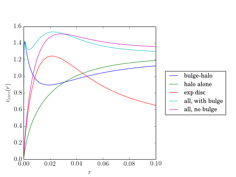
Figure 1: Circular velocity curve for halo and bulge (blue), the bulge-free halo model (green), the exponential disc (red), the combined model including the bulge (cyan), and the combined model without a bulge (magenta). The bulge is constructed to provide an approximately flat rotation curve in the inner galaxy. The bulge-free rotation curve rises inside of approximately two disc scale lengths.

3 Galaxy model and bar perturbation

We adopt the following set of $\Lambda$CDM units: the virial radius is the unit length scale and the mass of the dark matter halo inside the virial radius is unity. Scaled to the Milky Way, the unit mass is approximately $10^{12}M_{\odot}$ and the unit radius is $300\,\mbox{kpc}$. We model the bulge and spheroid by two NFW-like (Navarro, Frenk & White, 1997, NFW) profiles. To combine the dark-matter halo and bulge models, we “leave room” for the inner cusp by adding a core to the dark matter halo by adopting a modified NFW profile of the form

$$\rho(r)=\frac{\rho_{0}r_{s}^{3}}{\left(r+r_{c}\right)\left(r+r_{s}\right)^{2}}$$ (3)

where $r_{c}$ is zero for the original NFW profile. We consider a model with and without a bulge. For the model with a bulge, the dark-matter halo profile has a concentration of $c=15$ ($r_{s}=0.067$) and mass $M_{h}=1$ inside of $r=1$, with $r_{c}=0.02$. The bulge profile has a concentration of $c=3000$ ($r_{s}=0.000{\bar{3}}$) and a core radius $r_{c}=1.{\bar{6}}\times 10^{-5}$. This core radius limits the dynamic range of the density inside of any radius of astronomical interest here which simplifies some of the numerical computations. For the model without a bulge, the dark-matter halo profile has a concentration of $c=15$ ($r_{s}=0.067$) and mass $M_{h}=1$ inside of $r=1$, with $r_{c}=0.001$.

The two-dimensional disc is modelled by a thin exponential:

$$\Sigma(R)=\frac{M_{d}}{2\pi a^{2}}e^{-R/a}$$ (4)

The mass of the disc, $M_{d}$, was adjusted to produce an approximately flat circular velocity curve from zero to ten disc scale lengths. This mass is $M_{d}=0.04$ (approx. $4\times 10^{10}M_{\odot}$ scaled to the Milky Way). The scale length is chosen to be $a=0.01$ units (approx. $3\,\mbox{kpc}$ scaled to the Milky Way). The bulge mass is adjusted to keep the inner profile flat rather than rising. This gives a bulge mass 0.02 units ($2\times 10^{10}M_{\odot}$ scaled to the Milky Way) and a B/D ratio of 0.5. The bulge-free model has a rising rotation curve out to several disc scale lengths. The circular velocity profile for each component and the total for both models is shown in Fig. 1. Motivated by both observations and the results characterising many published n-body simulations, we chose the bar length to be that of disk scale length, $a_{1}=a$. Similarly, we choose pattern speed $\Omega_{p}$ so that the bar rotates at the same speed as a circular orbit at $R=a$.

Following previous contributions (e.g. Weinberg & Katz, 2002), we will model the bar as an ellipsoidal mass distribution. The gravitational potential for density stratified on ellipsoids is well known. Specifically, the gravitational potential internal to the ellipsoid takes the form (Chandrasekhar, 1969, pg. 52, eq. 93)

$$V=\pi Ga_{1}a_{2}a_{3}\int^{\infty}_{0}\frac{du}{\Delta}\left[\Psi(1)-\Psi(m^{2}(u))\right]$$ (5)

where

$$m^{2}(u)=\sum_{i=1}^{3}\frac{x_{i}^{2}}{a_{i}^{2}+u}$$ (6)

and

$$\Psi(m^{2})=\int_{1}^{m^{2}}dm^{2}\,\rho(m^{2}).$$ (7)

The gravitational potential external to the ellipsoid has the form (Chandrasekhar, 1969, pg. 51, eq. 89)

$$V=\pi Ga_{1}a_{2}a_{3}\int^{\infty}_{\lambda}\frac{du}{\Delta}\left[\Psi(1)-\Psi(m^{2}(u))\right].$$ (8)

We considered three different types of densities, power law, Ferrers (1887), and exponential:

$$\rho(m^{2}) = \rho_{0}\begin{cases}\left(1-\log m^{2}\right)&\mbox{if }\gamma=-1\\ \left(1-m^{2\gamma}\right)&\mbox{otherwise}\end{cases}$$

$$\rho(m^{2}) = \rho_{0}\left(1-m^{2}\right)^{\gamma}$$

$$\rho(m^{2}) = \rho_{0}\left(e^{-1/\gamma}-e^{m^{2}/\gamma}\right)$$

with $\gamma$ chosen to be physically sensible (i.e. $\gamma>=0$ for the first two cases and $\gamma$ of order the disc scale length in the final case). The resulting quadrupole was similar with all three models, and for ease, we choose to represent the bar with a homogeneous ellipsoid with axes $a_{1}=a=0.01,a_{2}=0.005,a_{3}=0.001$.

To simplify the numerical computation, we fit the resulting quadrupole to an analytic form which has the correct asymptotic power-law behaviour based on the multiple expansion of Poisson’s equation:

$$U_{22}(r)=b_{1}\frac{r^{2}}{1+\left(\frac{r}{b_{5}}\right)^{5}}$$ (9)

Fig. 2 compares the fit from equation (9) to the quadrupole component of equations (5) and (8). The power-law fit systematically exceeds the true value for small $r\ll 0.01$ but otherwise captures the run of $U_{22}$ in the vicinity of the bar end at 0.01 quite well.

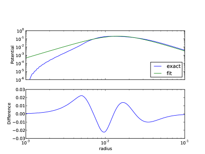
Figure 2: Comparison of the exact quadrupole potential $U_{22}(R)$ from the homogeneous ellipsoid and the power-law-type fit (eq. 9. The upper panel shows compares the fit in logarithmic units and lower panel shows the difference between the fit and the exact quadrupole.

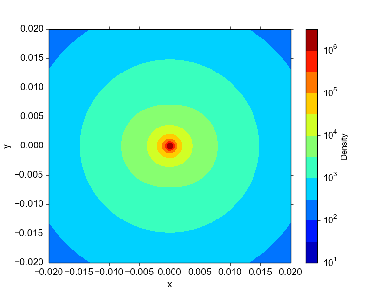
(a) $\epsilon=0.1$

(b) $\epsilon=0.3$

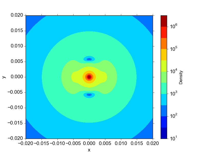
(c) $\epsilon=0.6$

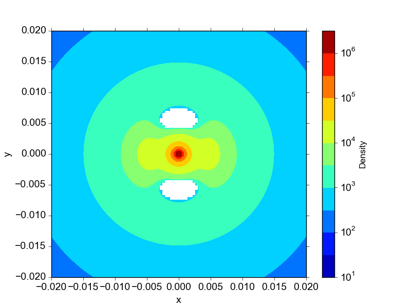
(d) $\epsilon=1.0$

Figure 3: Midplane density of the exponential disc with scale length $a=0.01$ (system units) including the bar perturbation for several amplitudes, $\epsilon$. The bar scale length equals the disc scale length, $a=0.01$.

Figure 4: Mapping of action space to orbit turning points for the unperturbed model shown on large (left) and small (right) scale. Loci of inner turning points (blue) and outer turning points (red) are labelled in system units. For reference, the bar length and disc scale length is 0.01 system units.

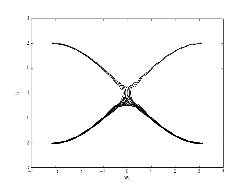
Figure 5: Twenty consecutive orbits from the two-resonance model from Paper 1 whose surface of section is illustrated section 4.1, Fig. 2 for an initial condition close to the homoclinic trajectory of the primary resonance. As the trajectory approaches the unstable equilibrium of the primary resonance at $(I_{1},w_{1})=(0,0)$, the oscillations induced by the secondary resonance weave back and forth across the homoclinic trajectory, leading chaotic behaviour.

4 Broken tori and chaos

In this section, we use the nKAM method developed in Paper 1 and the bar perturbation described in section 3 to determine the location and examine the morphology of broken tori. The approach is that same as that described for the Kepler example in Paper 1, section 5. The unperturbed model is the entire axisymmetric component: bulge, dark-matter halo and the exponential disc. The quadrupole fit to the triaxial ellipsoid representing the bar, described in the previous section, is the perturbation. Thus, the perturbation amplitude only affects the quadrupole strength. We assume a constant pattern speed $\Omega_{p}$ fixed to that of the circular orbit frequency at one disc scale length. As mentioned in section 2, it is possible to use the nKAM method to explore perturbations of finite duration; these will be tackled in a later contribution.

Since the actions are the fundamental description of the unperturbed phase space, we describe results of the nKAM procedure in the radial action–azimuthal action plane (that is, the $I_{1}$–$I_{2}$ plane) for a variety of bar quadrupole amplitudes. The fiducial mass in the triaxial ellipsoid that represents the bar is set equal disc mass enclosed within the bar radius. The resulting quadrupole amplitude is scaled to the desired bar strength. For visual comparison, Fig. 3 shows the midplane density implied by the quadrupole perturbation for four bar strengths spanning the range of interest. We use a logarithmic scaling for comparison with astronomical images and to better illustrate the bar amplitude near the ends of the bar. The full-amplitude ($\epsilon=1$) profile bears a close resemblance observed luminosity density for strong bars (e.g. Gadotti & de Souza, 2006). The negative-density “dimples” perpendicular to the bar that occurs for strongest amplitude case is an artefacts of only including the quadrupole term; higher-order multipole terms would fill in these regions perpendicular to the bar’s major axis. The potential and force remain physical even when dimple artefacts appear in the density profile. Fig. 3 further suggests that perturbations with $\epsilon\gtrsim 0.2$ are morphologically bar-like.

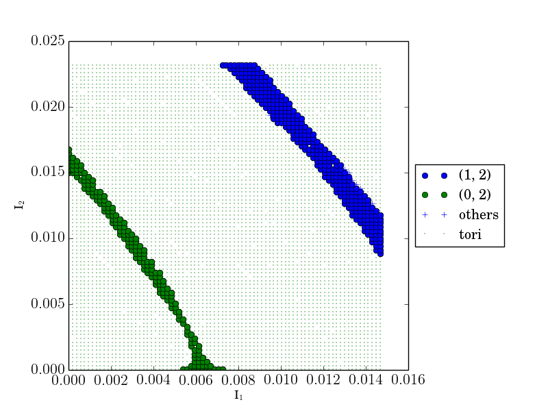
(a) $\epsilon=0.1$

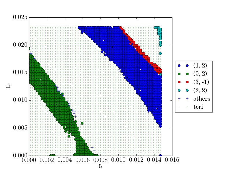
(b) $\epsilon=0.3$

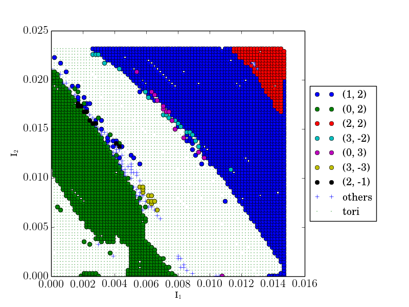
(c) $\epsilon=0.6$

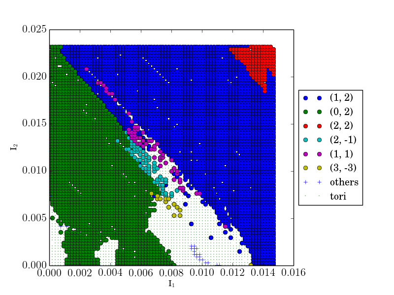
(d) $\epsilon=1.0$

Figure 6: Broken (good) tori are indicated by filled circles (dots) as a function of the unperturbed values of radial action $I_{1}$ and azimuthal action $I_{2}$ for the bulge-free galaxy model. The broken tori are colour coded by the principle resonance in the form $(l_{1},l_{2})$ (legend). For example $(-1,2)$ is the inner-Lindblad resonance and $(0,2)$ is the corotation resonance. Initially circular orbits like along the $I_{1}=0$ vertical line and initially radial orbits like along the $I_{2}=0$ horizontal line. The right-hand vertical axis describes the radius of the circular orbit ($I_{1}=0$) corresponding to each value of $I_{2}$.

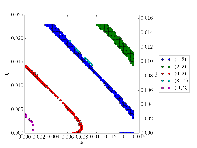
(a) $\epsilon=0.1$

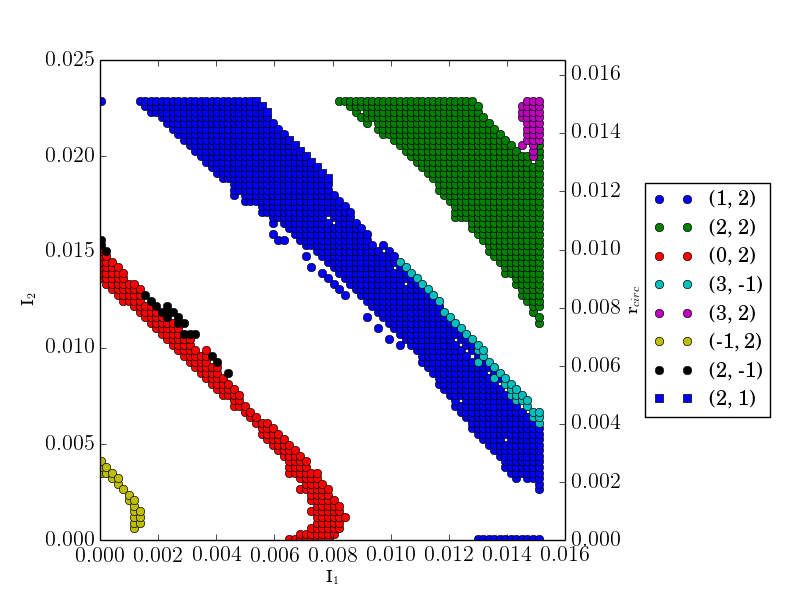
(b) $\epsilon=0.3$

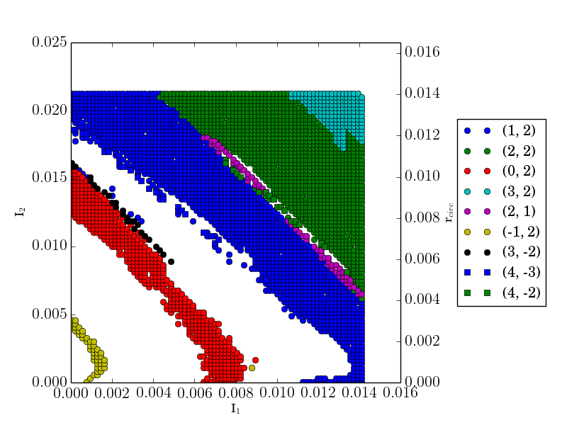
(c) $\epsilon=0.6$

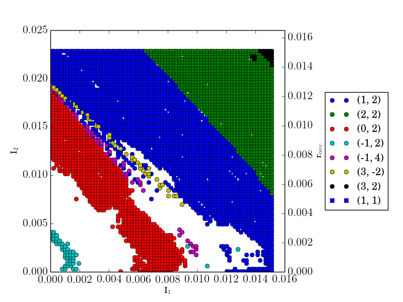
(d) $\epsilon=1.0$

Figure 7: As in Fig. 6 but for the galaxy model with a bulge and flat rotation curve.

The broken-tori action plots are shown in Figs. 6a–6d for the bulge-free, rising rotation curve model and in Figs. 7a–7d for model including a bulge with a relatively flat rotation curve. The sequence of panels in each figure corresponds to perturbation strength $\epsilon=0.1,0.3,0.6,1.0$. Each filled point denotes a broken torus; the colour key labels each by the term in the perturbation series (see Paper 1, eq. 16) with maximum amplitude. The loci of broken tori follow the low-order resonances, as expected. For example, the locus of broken tori at the lower-left in Fig. 6b follows the corotation resonance $(0,2)$, followed by the outer Lindblad resonance (OLR), $(1,2)$, moving to the upper right. By examining the coefficients in the generating-function series from Paper 1, eq. 16, we can identify the secondary resonance or combination of multiple secondary resonances implicated in splitting the separatrix of the primary resonance. In the case of the corotation resonance, the secondary resonances are most often the inner Lindblad resonance (ILR, $l_{1}=-1,l_{2}=2$), and vice versa for the primary ILR. For $\epsilon=0.1$ the relative strengths of the secondary-resonance coefficients $\varpi_{\mathbf{l}}$ of the $W_{1}$ series fall between 0.3% and 3%; these amplitudes seem to increase roughly linearly with increasing $\epsilon$. As the amplitude continues to increase, the width of the region near the locus of corotation, OLR, and ILR increase, starting to close the gap of unbroken tori between ILR and corotation available to support the bar figure. The main differences between the two series, Figs. 6a–6d and Figs. 7a–7d, are the locations and existence of various resonances. A flat rotation curve results in more resonances near and around vicinity of the bar, including the ILR at small radii.

We will see in section 4 below that the nKAM computation appears to underestimate the measure of stochastic orbits for mild eccentricity, typical of a disc, suggesting that a large fraction of orbits in the bar region are stochastic at some level. Indeed, computation of the SOS plots for in this region suggests most of the orbits in this region with near circular orbits, $I_{1}\ll I_{2}$, show some stochastic spreading. In many but not all cases, these irregular orbits appear to have inner and outer turning points although the envelope of the trajectory vary with time. This calculation is not self consistent so the we have no way of assessing whether the remaining unbroken tori are capable of reproducing the imposed gravitational perturbation. Nonetheless, the nKAM results suggest that a large fraction of the phase space in the bar vicinity is chaotic owing to bar itself. This raises the possibility that the bar amplitude and structure may be self-limited by stochasticity.

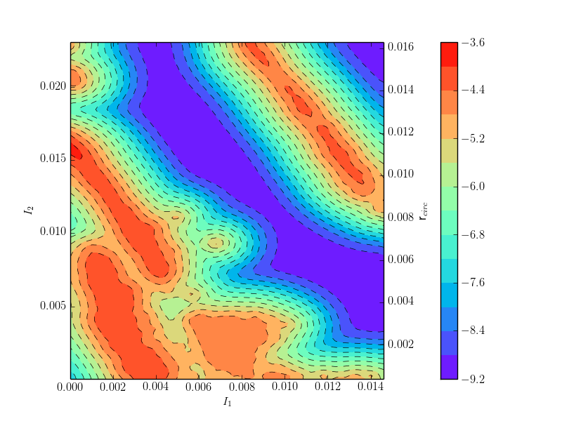
(a) $\epsilon=0.1$

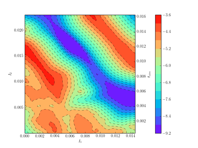
(b) $\epsilon=0.3$

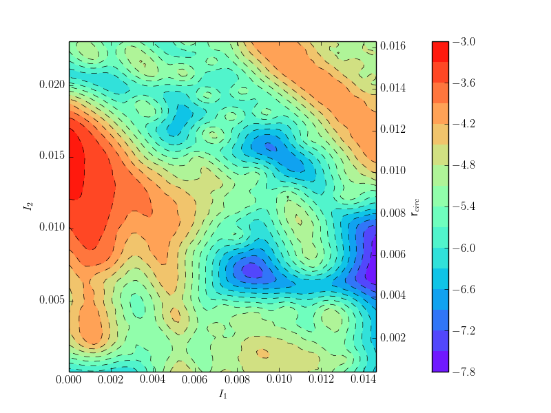
(c) $\epsilon=0.6$

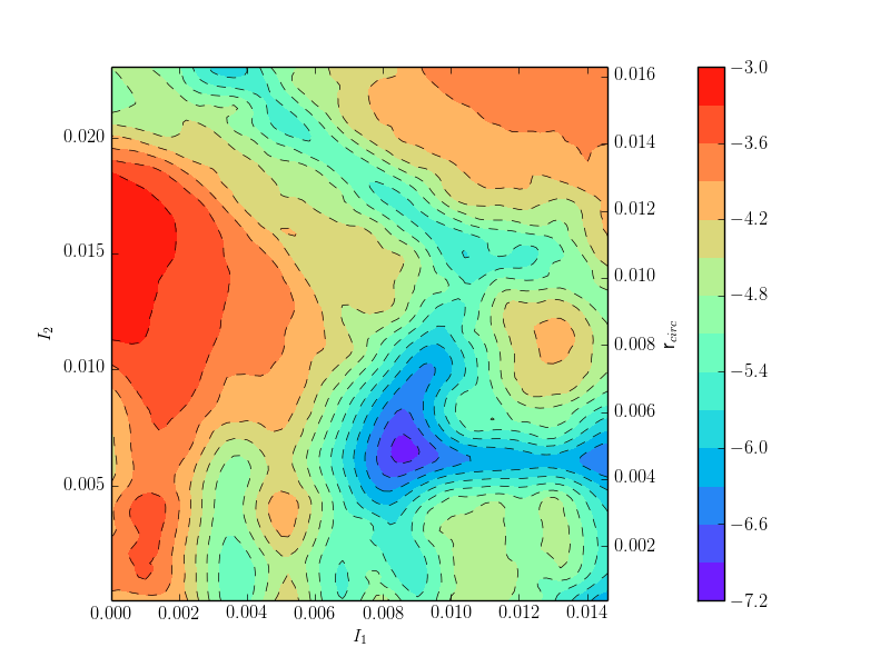
(d) $\epsilon=1.0$

Figure 8: Values of the largest (positive) Lyapunov exponents for models with various perturbation amplitudes for the bulge-free galaxy model. Positive Lyapunov exponents are determined by regression analysis to determine convergence with increasing time as described in Paper 1, section 3.2. The local estimate is computed by smoothing the ensemble onto a regular grid. Contour values are logarithmically spaced; values of $(I_{1},I_{2})$ that are converging to zero are shown in white.

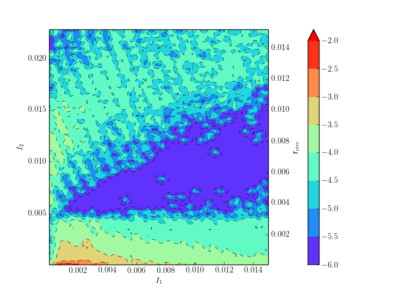
(a) $\epsilon=0.1$

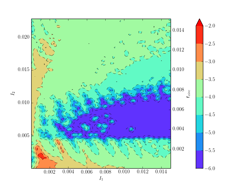
(b) $\epsilon=0.3$

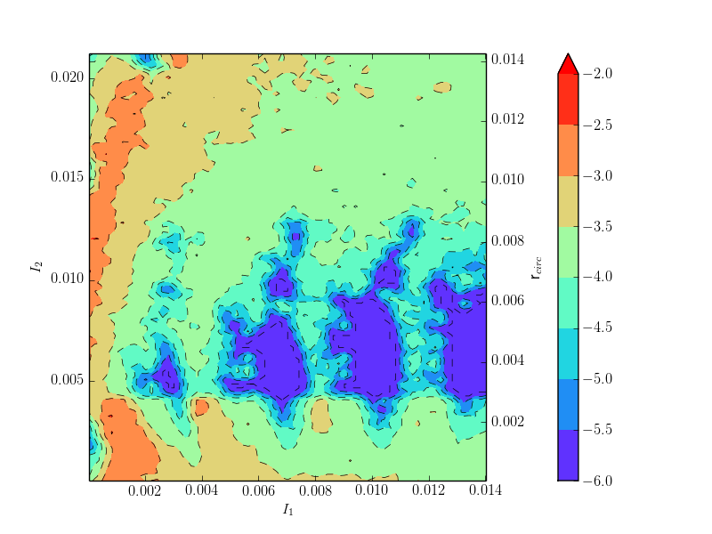
(c) $\epsilon=0.6$

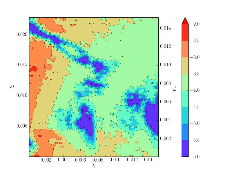
(d) $\epsilon=1.0$

Figure 9: As in Fig. 8 but for the galaxy model with a bulge and flat rotation curve.

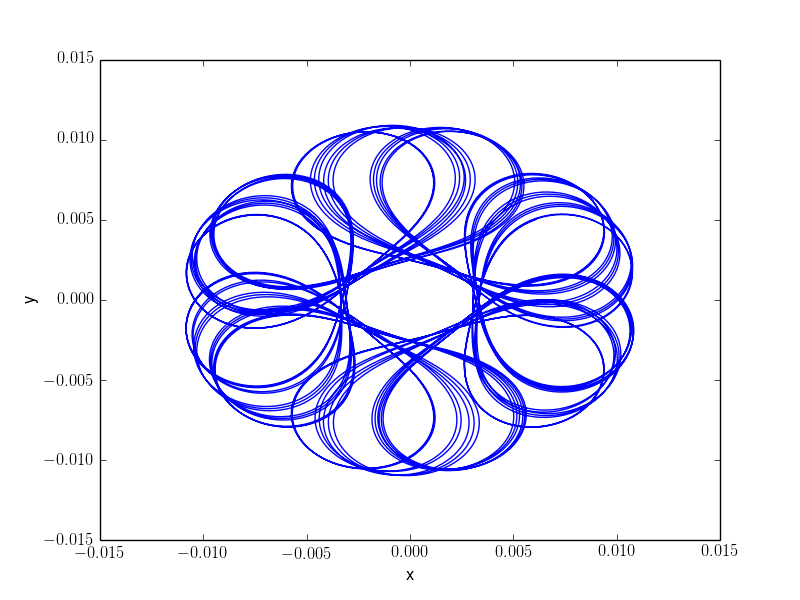
(a) regular zone, trajectory

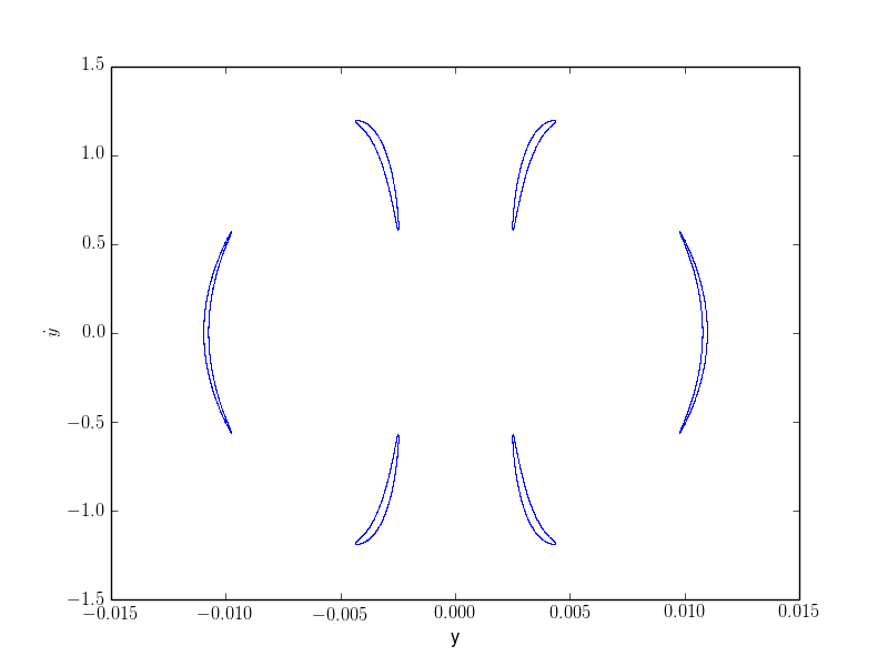
(b) regular zone, sos

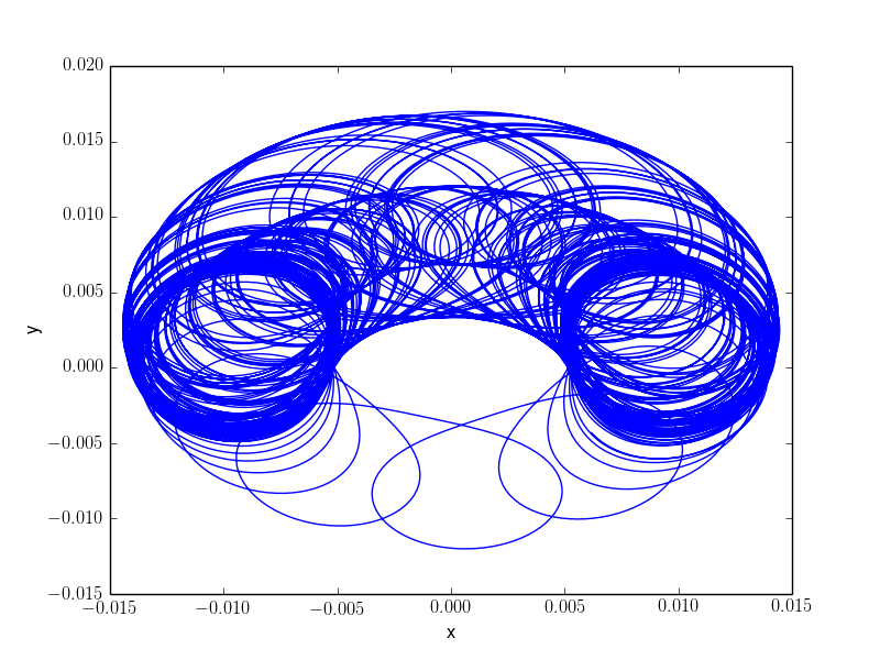
(c) chaotic zone, trajectory

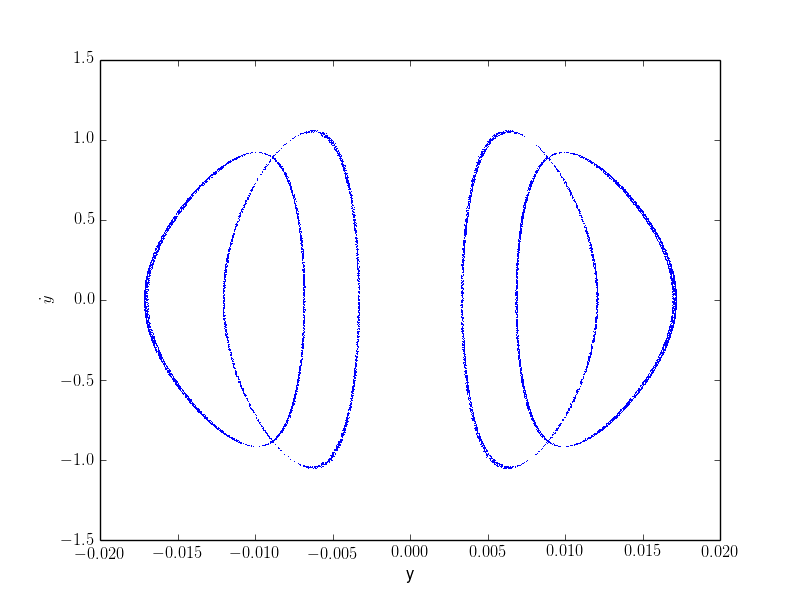
(d) chaotic zone, sos

Figure 10: Orbits shown in the frame rotating with the bar for $\epsilon=0.3$. The regular orbit constructed by the nKAM method has $(I_{1},I_{2})=(0.0025,0.007)$ and the chaotic orbit has $(I_{1},I_{2})=(0.0017,0.011)$. Both orbits have nearly the same Lyapunov exponent value: $\lambda\approx 2\times 10^{-5}$. The left-hand panels plot a short segment of the trajectory used to compute the two-sided SOS plots in the right-hand panels.

We now compare the results of a Lyapunov exponent analysis with nKAM predictions. The presence of a bulge adds an additional interpretive complication so we begin by describing the results for the bulge-free galaxy model with a rising rotation curve. The regions of positive Lyapunov exponent for the amplitudes in Figs. 6a–6d are depicted in Figs. 8a–8d. The locus of positive exponents and broken tori coincide approximately for the corotation and OLR resonances at all amplitudes. As the bar amplitude increases, corotation appears in positive Lyapunov values at high ($I_{1}\gtrsim I_{2}$) and low ($I_{1}\ll I_{2}$) eccentricity. Although the ILR does not appear as a primary resonance, it is a secondary resonance near the inner edge of the region of broken tori corresponding to the corotation resonance in all of Figs. 6a–6d. At lower amplitude, the ILR shows up as a distinct locus (Figs. 8a and 8b). At higher amplitude, regions of positive Lyapunov exponent owing to corotation and ILR blend together in a single locus (Figs. 8c and 8d).

For the flat rotation curve model, the regions of positive Lyapunov exponent for the amplitudes in Figs. 7a–7d are depicted in Figs. 9a–9d. For all amplitudes, we find a qualitative demarcation at $I_{2}\approx 0.004$, corresponding to orbits that move between the bulge and the disc (compare the rotation curve contributions in Fig. 1 with the turning point locations in Fig. 4). Resonances between the driving frequency of the bar and periods of control by the higher orbital frequencies of the bulge lead to the striations in Lyapunov exponent seen in these figures. The nKAM convergence has been checked by doubling and quadrupling the number of terms in the series, implying that high-order resonances are responsible for the striation. As the bar strength increases, the inner quadrupole, with a gravitational potential $\propto r^{2}$, strongly affects the bulge dynamics. The perturbation causes the location of these high-frequency striations to change location in action space with bar strength. In essence, the striations manifest in Figs. 9a–9d are a form of orbit “shocking.”

The locus of positive exponents and broken tori coincide approximately for the ILR at all amplitudes. SOS plots confirm that these orbits exhibit significant irregularity. As the bar amplitude increases, corotation appears in positive Lyapunov values at high ($I_{1}\gtrsim I_{2}$) and low ($I_{1}\ll I_{2}$) eccentricity. All in all, the overall conclusions for both galaxy models are qualitatively the same: increasing amplitude gives rise to an increasing fraction of stochastic orbits in the bar region. The galactic model with a flat rotation curve has a larger zone of unbroken tori that are bar supporting than the model with a rising rotation curve. For both models, the nKAM analyses predict a region at moderate eccentricity ($I_{1}\lesssim I_{2}$) just below the chaotic corotation regions where the orbits remain approximately regular in morphology and may support the bar. This zone of regularity decreases with increasing bar amplitude.

A major advantage of the nKAM approach is that it naturally provides a dynamical characterisation for the broken torus, i.e. hints to the primary and secondary resonances involved. On the other hand, a broken torus predicted by the KAM method does not predict the degree of exponential sensitivity. However, empirically, a ratio of secondary to primary amplitude of the generating function coefficients $\varpi_{\mathbf{l}}$ ( Paper 1, eq. 16) of order 0.1 or larger nearly always has a numerically measurable positive Lyapunov exponent. In essence, the secondary resonances break the forward and backward time symmetry of the stable and unstable branches of the resonant orbit. Chaos is induced by rapidly oscillating intersections of the perturbed stable and unstable manifolds in the sense of the Birkhoff-Smale theorem (Smale, 1965) that gives rise to exponential sensitivity. The resulting chaos is confined to a sheath surrounding the original unperturbed homoclinic trajectory (as in Holmes & Marsden, 1982). The dynamics of this behaviour was considered in detail by Wiggens (1990, Chapter 4). It can be easily seen numerically by plotting the solution of a direct numerical integration for the many resonance system in the action-angle space of the one-dimensional primary resonance near the homoclinic trajectory. For example, Fig. 5 shows a

The resulting motion for broken tori of this type remains generally confined in phase space. However, as the perturbation grows, the chaotic sheath can fill a large fraction of the original libration zone, which may be large. A typical orbit in this sheath appears to quickly vary its eccentricity; visually it presents as a rosette with turning points varying in radius with time.

This insight helps us interpret the differences between the approaches. Recall that the Lyapunov value indicates the exponential rate of divergence of two initial conditions. However, this does not describe the behaviour of the trajectory. Qualitative classification of orbital regularity by eye combined with the computation of SOS plots suggests significant irregularity for exponents with $\lambda={\cal O}(10^{-3})$. In many cases, the nKAM locus provides a more sensitive indicator of separatrix disruption than the Lyapunov exponent. For example, Fig. 10 depicts the trajectories and SOS plots for two orbits with the same value of $I_{1}$ and nearly the same value of Lyapunov exponent. One orbit is in the chaotic zone parented by corotation as predicted by the nKAM method, and one orbit is between the ILR and corotation chaotic zones [cf. Fig. 7b]. The orbit that is predicted to be regular by nKAM shows qualitatively regular features, and this is corroborated by the SOS plot. The orbit that is predicted to be chaotic by nKAM has two modes; the perturbation has broken the original torus resulting into two loop-like trajectories that joined at an unstable point. This behaviour is typical of broken tori in the corotation loci of Fig. 7 for $I_{1}\mathrel{\hbox to0.0pt{\lower 3.0pt\hbox{$\mathchar 536\relax$}\hss}\raise 2.0pt\hbox{$\mathchar 318\relax$}}I_{2}$. Broken tori with $I_{1}\ll I_{2}$ exhibit more complex behaviour, presumably from the superposition of effects from multiple secondary terms. This “mode switching” explains the qualitatively ‘chaotic’ appearance of trajectory but the small measured Lyapunov exponent values. Only near the hyperbolic point of the islands in the stochastic sheath does the exponential sensitivity to phase space play a strong role, and therefore, the time-averaged Lyapunov exponent can remain anomalously small in light of the qualitative stochastic behaviour of the trajectory over many periods.

In summary, each of these two methods, nKAM and Lyapunov exponent computation, reveal different aspects of irregular systems. The nKAM procedure identifies locations in phase space where influence of other nearby or strong resonances are capable of inducing morphological changes in near resonant orbits. Lyapunov-exponent analysis attempts to measure the rate of exponential sensitivity directly. This technique is good at discovering strong chaos but may miss subtle cases where the mild break up of a resonance into several islands that permits an orbit to spontaneously change morphologies after many dynamical times. In this later case, the trajectory is only exponentially sensitive to its initial conditions near an unstable point, and the time to transverse this critical region is a small fraction of its orbital time. While in this critical region, the orbit may change from one nearly regular morphology to another. In other words, the characteristic time scale for exponentiation, measured using the standard Lyapunov exponent algorithm, may be much longer than an a Hubble time but the broken torus can have a qualitatively different character owing to its tendency to switch between morphologies.

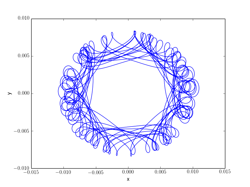
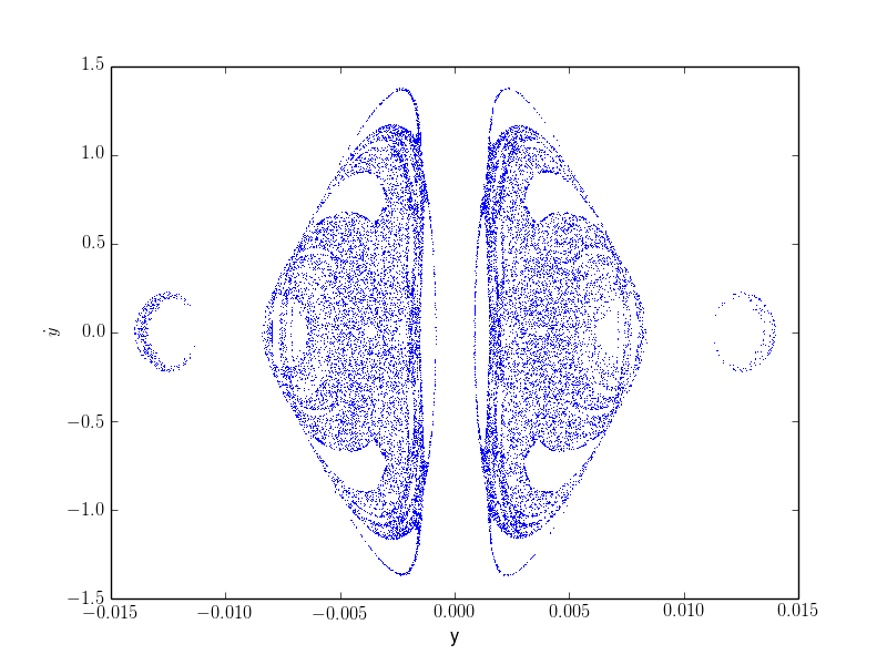
Figure 11: Orbit (left) and two-sided Poincaré SOS plot (right) for an initially nearly circular orbit with $(I_{1},I_{2})=(0.0004,0.011)$ at the middle of Lyapunov value plot for bar strength $\epsilon=0.3$ in Fig. 9b but outside the chaotic zone in Fig. 7b.

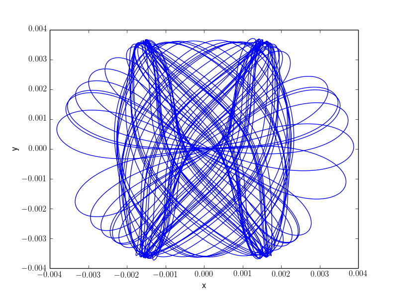
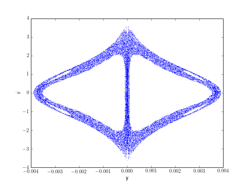
Figure 12: Orbit (left) and two-sided Poincaré SOS plot (right) for an initially mildly eccentric orbit with $(I_{1},I_{2})=(0.0002,0.004)$ in the chaotic zone predicted by the nKAM method. This orbit shows a broad stochastic sheath with significant turning point variation although the orbit does remain isolated.

The nKAM method does appear to underpredict the stochastic regions. Indeed, many of the orbits with $I_{1}<0.001$ and $0.010<I_{2}<0.015$ that show larger values of Lyapunov exponent in Fig. 9 exhibit the qualitative signature of chaos, although the nKAM method is able to construct a torus. Choosing a specific example from the $\epsilon=0.3$ model, Fig. 11 describes an initially nearly circular orbit with $(I_{1},I_{2})=(0.0004,0.011)$, which is near the middle of the higher Lyapunov value band near the corotation resonance. The origin of this discrepancy is not clear. Increasing the number of nodes in Fourier series by factors of 4 and 16 do not change the loci of broken tori significantly. More likely, as in the standard application of the KAM theorem, the quadratically convergent algorithm appears to robustly find tori in the vicinity of broken tori whenever possible. That is, away from the vanishing denominators, the iterative algorithm tends toward a solution if at all possible. This suggests that the nKAM procedure is conservative: it will find regular orbits if they are in a small neighbourhood of the specified initial condition even if irregular orbits can be found there as well. Conversely, the Lyapunov exponent procedure seems to find both regular and irregular orbits in the same neighbourhood, if the both exist, and possibly switches between them (more on this below).

A second limitation of the nKAM procedure using the fundamentally linearised solution of the HJ equation is its intrinsically perturbative nature. So, it is possible that nKAM method has been pushed beyond its domain of accuracy for this problem resulting in the underprediction of stochasticity in this case. For larger value of $I_{1}$, the nKAM appears to be a sensitive indicator of weak or confined (e.g. Dvorak et al., 1998; Winter, Mourão & Giuliatti Winter, 2010) chaos, perhaps as expected, than the Lyapunov exponent value. However, the different characterisations persist even for $\epsilon\lesssim 0.2$, and therefore, so strong non-linearity is not the full explanation.

For another example, Fig. 12 shows the same plots as Fig. 10 for a chaotic orbit in the ILR region. Upon increasing $I_{2}$ at fixed $I_{1}$ beyond the locus of nKAM-predicted broken tori, the SOS continues to exhibit significant width, suggesting that the nKAM method underestimates the measure of broken tori here as well. Decreasing the amplitude of the perturbation reveals the bifurcations and islands expected of a stochastic layer; the trajectory appears regular over short times but can switch between different regular morphologies. This reinforces our previous interpretation for the discrepancy between the apparently small values of Lyapunov exponent when the orbit appears irregular overall: the stickiness in the stochastic sheath results in regular behaviour punctuated by jumps to different parent resonances near islands. One may easily verify there is clear structure in the SOS over short finite-time periods that blends together over long periods.

5 Summary and discussion

5.1 The method

In this paper, we using the numerical KAM (nKAM) method described in Weinberg (2015a) to explore the location and frequency of tori broken by a Galactic-bar perturbation. In essence, this technique predicts the existence of regular orbits (which have three actions) and irregular orbits (with fewer than three actions) by an iterative solution of the linearised Hamilton-Jacobi (HJ) equation. The HJ equation defines a canonical transformation to the action-angle variable system, and we assume that a consistent solution for the canonical formation implies existence and vice versa. In section 4, we show that the nKAM computation yields useful predictions predictions for regions of irregularity, however, the method underpredicts the width of the chaotic zones for strong bars. This trend may be understood as follows. The nKAM method appears to find a torus if one exists in the neighbourhood of the initial conditions, even if broken tori exist in this same neighbourhood. Conversely, the Lyapunov method tends to find exponential divergence in the same circumstances, if it exists, although orbits may switch behaviour suddenly, e.g. if the initially diffusing trajectory encounters a regular island. These differences are not expected, but further elucidate that chaos is a broad catch-all term for orbits with a wide variety of irregular morphology.

Thus, the two approaches reveal different information about the same problem. The nKAM provides dynamical details about the principle and secondary resonances for broken tori although the method is less accurate for strong perturbations owing to its perturbative nature. The Lyapunov analysis works for any perturbation, but the dynamical origin of a positive Lyapunov exponent is not readily available. Moreover, our investigation suggests that Lyapunov exponent analysis does not provide useful information about stochastic orbits that appear isolated to stochastic layers. The morphology of the orbits within these layers often exhibit large variance in orbital frequencies while yielding the anomalously small Lyapunov exponents typical of weak chaos. Since the morphology of orbits as measured by their time-averaged density is key to understanding the evolution of patterns such as arms and bars, an random switching between families matters. This suggests that Lyapunov analysis may have less value for some important galactic dynamics problems. In addition, the nKAM is capable of providing a new action-angle coordinate system for those tori that survive a perturbation, although we do not exploit this feature in the present paper. Conversely, the nKAM method does not provide a direct assessment of the magnitude of the chaos without additional analysis; e.g. strong chaos may be inferred from the relative magnitude of coefficients in $\varpi_{\mathbf{l}}$ using the Chirikov (1979) criterion.

Our conclusion from this work is that galactic evolution under the influence of strong patterns (bars, spiral arms, etc.) has an important chaotic component. As described in section 1, this conclusion has been reached by previous researchers as well. Although standard perturbation theory provides some physical insight, it is necessarily an incomplete picture of the underlying dynamics. We have some hope that the extended perturbation theory described above may provide a bridge between analytic methods and unencumbered n-body simulation. Numerically, much of our motivation for criteria for orbit integration stems from the study of regular orbits.

5.2 Implication for bars

In addition to characterising the new method, our main goal is a study of the degree of stochasticity induced by a stellar bar in an initially axisymmetric galaxy disc. The importance of weak chaos in structuring stable orbits under non-axisymmetric perturbations and the underlying dynamics is nicely illustrated by Romero-Gómez et al. (2006, 2007); Athanassoula, Romero-Gómez & Masdemont (2009) who describe the importance of weak chaos in creating rings in barred galaxies. Their dynamical description of orbit transitions at unstable points is essentially that described in section 4 (Fig. 10d and associated discussion.). There are, of course, other approaches. For example, Bountis, Manos & Antonopoulos (2012) describe a probabilistic approach that simultaneously discriminates between weak and strong chaos. An advantage of the nKAM approach is that it provides a numerical tool for a wholesale investigation of phase space as a in a computationally efficient way. At the same time, it produces a multiple-resonance model Hamiltonian to further investigate broken tori.

Based on an action-space expansion, our nKAM investigation provides a provides a statistical view of irregularity caused by a perturbation or pattern. We assumed an analytic bar model and examined the influence of its quadrupole moment on the disc. The bar here is modelled by a homogeneous ellipsoid with the axis ratio and density profile typical of observed bars (see section 3). The bar does not evolve with time or is it self-consistent in any way; this is an idealisation that makes this present investigation tractable, although extensions with more generality are possible. The key findings are as follows:

1. The principle resonances causing broken tori in the inner galaxy are the corotation $(0,2)$ and the OLR $(1,2)$ resonances. The secondary resonances with the largest amplitude for corotation are ILR $(-1,2)$ and OLR $(1,2)$; their amplitude relative to the primary resonance is roughly 3% for a strong bar. The strongest-amplitude secondary resonance for OLR is $(2,2)$; their amplitude relative to the primary is roughly 10%.

2. It may seem strange that major low-order resonances affect each other. However, for a strong bar perturbation, i.e. when the non-axisymmetric force is similar in magnitude to the axisymmetric force, the width of libration zones for these resonances are comparable to the actions themselves.

3. As the amplitude increases, approaching that of a strong bar, many orbits in the vicinity of bar become chaotic, leaving a small phase-space region of modestly eccentric non-chaotic orbits between the ILR and corotation resonances. This the same part of phase space responsible for supporting the bar itself (e.g. Contopoulos & Papayannopoulos, 1980). This suggests that bar strength may be limited by the chaos induced by the bar itself, preventing further growth.

4. The Lyapunov exponent values do not accurately diagnose the chaos caused by the stochasticity sheaths that form around primary resonances. The use of these exponents may provide a biased assessment of irregularity for galactic dynamics.

5.3 Implications for n-body simulations

As described by Chirikov (1979), in Paper 1 section 4.1, and in the previous sections of this paper, non-deterministic behaviour owing to mutual interaction of resonances gives rise to a sheath of chaotic behaviour around the primary resonance. In perturbation theory based on the averaging principle, we isolate the degree of freedom corresponding to a resonance by examining its dynamics close to its (unstable) homoclinic trajectory. The phase frequency corresponding to this degree of freedom will be small and we call the corresponding action the slow action. The slow action corresponding to this homoclinic trajectory of the primary resonance will be, in general, a linear combination of the actions defined by the separable coordinates of the unperturbed background potential. Therefore, motion in this sheath can result in changes of the original actions of order the width of the libration zone.

For the specific example explored in section 4, chaotically induced switching of orbit families occurs in regions of very small phase-space volume near unstable points. The pervasiveness of this fine-scale structure in phase space induced by chaos motivates a technical campaign to determine sufficient conditions on n-body simulation necessary to accurately recover the important consequences of the mixed regular and irregular dynamics of galaxies. Typical time-step selection algorithms for n-body simulations choose a fraction of the rate of change of position or velocity of a trajectory in its gravitational field. The scale of the gravitational field may be determined by examining the derivative of forces or from prior knowledge about the desired resolution length scale. However, the dynamics of interacting resonances is sub-dimensional. Therefore, the details of the dynamics around the primary resonance may require the resolution of scales much smaller than those characteristic of the trajectory as a whole. For example, if a single step in the ODE solver moves the orbit through the chaotic zone altogether, the chaotic dynamics may disappear from the simulation. Indeed, accurate computation of the Lyapunov exponents in Paper 1 section 3.2 suggest that the required time steps are much smaller than those chosen for n-body simulations; larger time steps resulted in negative rather than positive exponents in many cases. Similar issues were seen in the computation of SOS plots for section 4. The topology of the SOS plots for broken tori are often not converged until time steps are several orders of magnitude smaller than the characteristic orbital times for the RK4 time stepper.

5.4 Future work

Many of our analytic tools for studying modes and secular processes excited by bars and strong spiral patterns are based on the existence of regular orbits. Our success in studying the statistical implication of an imposed pattern as described in section 5.2 leads to a secondary longer-term goal: can we extend perturbation theory methods to understand and predict the long-term future of secularly evolving galaxies that includes the effects of chaos?

Indeed, an immediate consequence of the unbroken tori found using nKAM is a new basis for secular perturbation theory. The framework described in Paper 1 and in section 2 provides the new regular trajectories in an action-angle representation when they exist. This basis may be used to estimate bar kinematic signatures, perform stability analyses, and so on; any task previously performed using Hamiltonian perturbation theory may be performed using the new action-angle representation. This naturally allows the standard tools of secular perturbation theory (i.e. Tremaine & Weinberg, 1984) to be used in the mixed context of regular and irregular orbits. Of course, this only makes sense if many of the tori remain unbroken. Based on the results of section 4, this roughly true for all but the strongest bars.

The orbit morphology in the perturbed regions may be significantly different than the unperturbed one. For example, Fig. 10a describes an regular orbit reconstructed by the nKAM method. The SOS plot [Fig. 10d] reveals that the simple rosette orbit has been destroyed and replaced with an orbit whose turning points are trapped by the rotating bar potential. These changed morphologies of nKAM-determined regular orbits are capable of supporting new classes of responses not possible with the original unperturbed regular system. For Fig. 10c, the new orbit may still be bar supporting, but less so than a classical x1 bar orbit from Contopoulos & Papayannopoulos (1980). In addition, each new class of regular orbits is likely to present a different kinematic signature than the original unperturbed orbit, and an ensemble chosen to represent the bar may be used to predict kinematic signatures.

A companion paper applies the nKAM method to a three-dimensional but axisymmetric system. A natural extension of this work to three dimensions would explore the role stochasticity in coupling between the planar and vertical degrees of freedom. For some examples of the questions to be addressed, does the bar perturbation drive disc thickening through stochastic means? Do broken tori play a role in producing a pseudo-bulge? As described in Paper 3, the fully asymmetric three-dimensional implementation of the nKAM method is computational challenging but surmountable. Each torus is represented by several three-dimensional Fourier series describing the canonical generating function and tables of the unperturbed orbits as a function of angles. The numerical partial derivatives required by the nKAM method requires that three-dimensional action cube be finely sampled by these tori. This leads to a large RAM requirement. The current code parallelises torus computation and shares the results with all processes. A redesigned code would use an action-space domain decomposition to eliminate need for each compute node have a full copy of the Fourier series and angles grids for each torus. This will allow a computationally feasible, general, three-dimensional nKAM code.

The example here assumes the simplest quasi-periodic time-dependent perturbation: one with a single constant pattern speed. As described in Paper 1 and sections above, the nKAM method may be extended to include general time-dependent perturbations by breaking down the time-dependent perturbation using a Fourier (or Laplace) series approximation. A related question is the effect of the slow evolution of the bar and background gravitational field owing to secular torques. For example, does the slow evolution increase or decrease the size and effects of the stochastic layers? Naively, the effective frequency of the slow evolution is much smaller than the orbital frequencies in the inner galaxy, and this makes the coupling between the natural frequencies and the evolution frequencies weak. Conversely, the low spatial frequency of the secular evolution may effectively couple to the primary perturbation for a strong bar, providing new channels for separatrix breaking. Moreover, the existence of chaos in the vicinity of orbits supporting the bar is likely to affect capture into libration. For example, since bars are formed by capture into libration, we might expect diffusion in and out of the libration zone as the bar pattern speed changes. Results from section 4 suggest that stochastic regions caused by the forming and growing bar increase with bar strength. Understanding influence of slow evolution on stochasticity from first principles and the possibility that bars are chaotically self-limited is the next challenge.

References

- Arnold (1963) Arnold V. I., 1963, Russian Mathematical Surveys, 18, 13
- Athanassoula et al. (2009) Athanassoula E., Romero-Gómez M., Bosma A., Masdemont J., 2009, Monthly Notices of the Royal Astronomical Society, 400, 1706
- Athanassoula, Romero-Gómez & Masdemont (2009) Athanassoula E., Romero-Gómez M., Masdemont J., 2009, Monthly Notices of the Royal Astronomical Society, 394, 67
- Benettin et al. (1980) Benettin G., Galgani L., Giorgilli A., Strelcyn J. M., 1980, Meccanica, 15, 9
- Binney & Tremaine (2008) Binney J., Tremaine S., 2008, Galactic Dynamics: (Second Edition) (Princeton Series in Astrophysics). Princeton University Press
- Bountis, Manos & Antonopoulos (2012) Bountis T., Manos T., Antonopoulos C., 2012, Celestial Mechanics and Dynamical Astronomy, 113, 63
- Brunetti, Chiappini & Pfenniger (2011) Brunetti M., Chiappini C., Pfenniger D., 2011, A&A, 534, A75
- Cachucho, Cincotta & Ferraz-Mello (2010) Cachucho F., Cincotta P. M., Ferraz-Mello S., 2010, Celestial Mechanics and Dynamical Astronomy, 108, 35
- Caranicolas & Zotos (2013) Caranicolas N. D., Zotos E. E., 2013, Publ. Astron. Soc. Australia, 30, 49
- Chandrasekhar (1969) Chandrasekhar S., 1969, Ellipsoidal Figures of Equilibrium. Yale University Press, New Haven
- Chirikov (1979) Chirikov B. V., 1979, Physics Reports, 52, 265
- Contopoulos (2002) Contopoulos G., 2002, Order and chaos in dynamical astronomy. Order and chaos in dynamical astronomy /George Contopoulos. Berlin : Springer, c2002. (Astronomy and astrophys library) QB 351 .K58 2002
- Contopoulos & Harsoula (2010) Contopoulos G., Harsoula M., 2010, Celestial Mechanics and Dynamical Astronomy, 107, 77
- Contopoulos & Papayannopoulos (1980) Contopoulos G., Papayannopoulos T., 1980, A&A, 92, 33
- Cvitanović et al. (2012) Cvitanović P., Artuso R., Mainieri R., Tanner G., Vattay G., 2012, in Chaos: Classical and Quantum, verstion 14 edn., Niels Bohr Institute, Copenhagen, pp. 114–124
- Dvorak et al. (1998) Dvorak R., Contopoulos G., Efthymiopoulos C., Voglis N., 1998, Planet. Space Sci., 46, 1567
- Ferrers (1887) Ferrers N. M., 1887, Quart. J. Pure Appl. Math, 14, 1
- Foster (1995) Foster I., 1995, Designing and Building Parallel Programs: Concepts and Tools for Parallel Software Engineering. Addison-Wesley
- Gadotti & de Souza (2006) Gadotti D. A., de Souza R. E., 2006, ApJS, 163, 270
- Giordano & Cincotta (2004) Giordano C. M., Cincotta P. M., 2004, A&A, 423, 745
- Goldstein, Poole & Safko (2002) Goldstein H., Poole C. P., Safko J., 2002, Classical Mechanics, 3rd edn. Addison-Wesley
- Harsoula, Kalapotharakos & Contopoulos (2011) Harsoula M., Kalapotharakos C., Contopoulos G., 2011, MNRAS, 411, 1111
- Holmes & Marsden (1982) Holmes P., Marsden J. E., 1982, Comm. Math. Phys. 82 523 (1982), 82, 523
- Kaufmann & Contopoulos (1996) Kaufmann D. E., Contopoulos G., 1996, A&A, 309, 381
- Kolmogorov (1954) Kolmogorov A., 1954, The Proceedings of the USSR Academy of Sciences, 98, 527–530
- Laskar (1990) Laskar J., 1990, Icarus, 88, 266
- Manos (2008) Manos A., 2008, PhD thesis, Universit/’e de Provence, France and University of Patras, Greece
- Manos & Athanassoula (2011) Manos T., Athanassoula E., 2011, Monthly Notices of the Royal Astronomical Society, 415, 629
- Manos & Machado (2014) Manos T., Machado R. E. G., 2014, MNRAS, 438, 2201
- Moser (1962) Moser J., 1962, Nachrichten der Akademie der Wissenschaften in Göttingen, Mathematisch-Physikalische Klasse, 1
- Moser (1966) Moser J., 1966, Annali della Scuola Normale Superiore di Pisa, Ser. III, 20, 499
- Navarro, Frenk & White (1997) Navarro J. F., Frenk C. S., White S. D. M., 1997, ApJ, 490, 493
- Patsis, Athanassoula & Quillen (1997) Patsis P. A., Athanassoula E., Quillen A. C., 1997, ApJ, 483, 731
- Romero-Gómez et al. (2007) Romero-Gómez M., Athanassoula E., Masdemont J. J., García-Gómez C., 2007, A&A, 472, 63
- Romero-Gómez et al. (2006) Romero-Gómez M., Masdemont J. J., Athanassoula E., García-Gómez C., 2006, A&A, 453, 39
- Shimada & Nagashima (1979) Shimada I., Nagashima T., 1979, Prog. Theor. Phys., 61, 1605
- Smale (1965) Smale S., 1965, in Differential and Combinatorial Topology (A Symposium in Honor of Marston Morse), Princeton University Press, Princeton, N.J., p. 63–80
- Tremaine & Weinberg (1984) Tremaine S., Weinberg M. D., 1984, MNRAS, 209, 729
- Tsoutsis et al. (2009) Tsoutsis P., Kalapotharakos C., Efthymiopoulos C., Contopoulos G., 2009, A&A, 495, 743
- Weinberg (2015a) Weinberg M. D., 2015a, MNRAS, paper 1, submitted
- Weinberg (2015b) Weinberg M. D., 2015b, MNRAS, paper 3, submitted
- Weinberg & Katz (2002) Weinberg M. D., Katz N., 2002, ApJ, 580, 627
- Wiggens (1990) Wiggens S., 1990, Introduction to Applied Nonlinear Dynamical Systems and Chaos, Texts in Applied Mathematics. Springer
- Winter, Mourão & Giuliatti Winter (2010) Winter O. C., Mourão D. C., Giuliatti Winter S. M., 2010, A&A, 523, A67
- Wolf et al. (1985) Wolf A., Swift J. B., Swinney H. L., Vastano J. A., 1985, Physica, 16D, 285
- Zaslavsky (2007) Zaslavsky G. M., 2007, The Physics of Chaos in Hamiltonian Systems. Imperial College Press