How to obtain thermostatted ring polymer molecular dynamics from exact quantum dynamics and when to use it

Abstract

We obtain thermostatted ring polymer molecular dynamics (TRPMD) from exact quantum dynamics via Matsubara dynamics, a recently-derived form of linearization which conserves the quantum Boltzmann distribution. Performing a contour integral in the complex quantum Boltzmann distribution of Matsubara dynamics, replacement of the imaginary Liouvillian which results with a Fokker-Planck term gives TRPMD. We thereby provide error terms between TRPMD and quantum dynamics and predict the systems in which they are likely to be small. Using a harmonic analysis we show that careful addition of friction causes the correct oscillation frequency of the higher ring-polymer normal modes in a harmonic well, which we illustrate with calculation of the position-squared autocorrelation function. However, no physical friction parameter will produce the correct fluctuation dynamics for a parabolic barrier. The results in this paper are consistent with previous numerical studies and advise the use of TRPMD for the computation of spectra. This manuscript has been submitted to Molecular Physics. If accepted for publication, it will be available at http://wwww.tandfonline.com

I Introduction

The computation of thermal time-correlation functions is of central importance in chemical physics gar09 ; zwa01 in order to evaluate many physically observable quantities such as reaction rates, diffusion constants, spectra and scattering data. hab13 ; liu15

Exact evaluation of the quantum correlation function scales exponentially with system size and so is impractical for more than a few atoms. hab13 There is consequently a need for computationally tractable approximations to quantum time-correlation functions liu15 ; mil05rev , preferably which are known to be equivalent to the quantum result in certain limits, and for which the likely error is known in advance of calculation. One crude solution is to use a purely classical correlation function, which will scale linearly with system size. However, the classical Boltzmann distribution is highly inaccurate for many systems such as water at room temperature hab09 , and ignores effects such as tunnelling and zero-point energy. hab13 ; mil05rev There is consequently a need to incorporate quantum statistics into such calculations, but with approximate, preferably classical-like, dynamics.

Various approaches have been developed, including the “classical Wigner” or linearized semiclassical initial value representation (LSC-IVR) method wig32qm ; liu15 ; liu07 ; shi03 which truncates the (exact) Moyal series moy49 for time evolution at $\hbar^{0}$, Centroid Molecular Dynamics (CMD) cao94_1 ; cao94_2 ; cao94_3 ; cao94 ; cao94_5 ; vot96 ; kin98 ; rei00 , which propagates the path-integral centroid in the mean-field of the other path-integral normal modes, and Ring Polymer Molecular Dynamics (RPMD) man04 ; man05che ; man05ref ; hab13 which takes the classical dynamics of a ring polymer par84 literally.

All these methods have various limitations; LSC-IVR does not conserve the quantum Boltzmann distribution leading to zero-point energy leakage hab09 ; liu15 , whereas CMD and RPMD both fail for multidimensional spectra wit09 ; iva10 ; CMD has the curvature problem where peaks are broadened and red-shifted whereas RPMD has spurious resonances where the ring polymer springs couple to frequencies in the potential leading to splitting of the physical peak. ros14

Recently, Thermostatted Ring Polymer Molecular Dynamics (TRPMD) has been introduced, which applied a Langevin thermostat cer10phd ; nit06 ; bus07 to the dynamics of the ring polymer cer10 ; ros14 ; ros14com . This was originally conceived for the evalutation of static properties cer10 , but it appeared to be remarkably successful for the computation of spectra ros14 ; ros14com , accurately replicating multidimensional spectra where CMD and RPMD fail and correctly predicting the diffusion and rotational constants of liquid water. Like RPMD, the short-time, transition-state theory (TST) limit of the TRPMD flux-side correlation function is identical to quantum transition-state theory (QTST) ros14 ; hel13 ; alt13 ; hel13unique ; hel14phd : the instantaneous thermal ring-polymer flux through a position-space dividing surface is equal to the intantaneous thermal quantum flux, and the TRPMD rate will equal the exact quantum rate in the absence of recrossing by either the quantum dynamics or TRPMD dynamics alt13 . Because TRPMD obeys detailed balance, its reaction rate is independent of the location of the dividing surface hel15trpmd , as is the case for RPMD and CMD but not many TST-based methods.

Nevertheless, TRPMD is not without its faults; like RPMD and CMD it fails to capture effects such as a Fermi resonance involving a fourth-order coupling in the Zundel cation ros14 , and beneath the crossover temperature (see Eq. (29)) application of friction to reaction rates causes them to decrease, resulting in a less accurate result compared to RPMD for symmetric systems, and a more accurate result (but with an adjustable parameter whose value is not determinable in advance) for asymmetric systems. hel15trpmd

Very recently, both RPMD and CMD have been obtained from the exact quantum time-correlation function via “Matsubara dynamics”, a form of linearization which conserves the quantum Boltzmann distribution hel15 ; hel15rel . Matsubara dynamics results from discarding fluctuations of the very high frequency path-integral normal modes (higher frequencies than those required to converge the quantum Boltzmann distribution) from the (exact) Moyal bracket and is inherently classical as well as satisfying detailed balance hel15 . However, Matsubara dynamics is not amenable to computation in large systems since it suffers from the sign problem due to a phase factor in the complex quantum Boltzmann distribution hel15rel . An approximation to Matsubara dynamics where the centroid moves in the mean field of the other Matsubara modes leads to CMD, and by moving the momentum contour in the quantum Boltzmann distribution and discarding the imaginary Liouvillian which results, RPMD arises hel15rel .

Obtaining RPMD and CMD from the exact quantum expression provides analytical expressions for their error from the quantum result, such that it can be known a priori whether they will function well in a given system, whereas previously one had to rely on induction from earlier numerical studies on systems for which RPMD or CMD had been successful, though there was no guarantee that such reasoning would extend to a new system. This was seen, for example, in RPMD rate theory failing in the Marcus inverted regime men11 despite being very successful for rate computation in a large variety of other systems man05che ; man05ref ; col09 ; col10 ; sul11 . With the derivation of QTST hel13 ; alt13 ; hel13unique ; hel14phd , it can be known a priori that a system whose optimal ring-polymer dividing surface will be significantly recrossed by the quantum dynamics will not have its rate accurately computed by RPMD hel14phd .

Consequently, investigating whether TRPMD could also be obtained from exact quantum time evolution and thereby discerning the situations where it is likely to work a priori, rather than relying on the (small but growing) literature of its application to physical systems ros14 ; ros14com ; hel15trpmd , would be of considerable benefit to the field.

In this paper we obtain TRPMD from exact quantum dynamics by showing that it is a stochastic approximation to Matsubara dynamics. To obtain a computationally tractable approximation to Matsubara dynamics, we move the momentum contour in the complex plane in order to convert the complex quantum Boltzmann distribution into the real ring polymer distribution. This transformation generates a complex Liouvillian in the dynamics hel15rel , which is not in itself amenable to computation due to the complex trajectories which result. Previously, the imaginary part of the Liouvillian was simply discarded, shifting the oscillation frequencies in the higher normal modes and leading to RPMD, but here we replace it with a Fokker-Planck term, producing TRPMD.

To examine the effect of the friction matrix we conisder a harmonic well and a parabolic barrier, for which the correlation function (if defined) can be evaluated analytically. We find that a unique and system-independent value of the friction matrix causes all normal modes to oscillate at the correct (external) frequency in a harmonic well, and illustrate this with the position-squared autocorrelation function, where TRPMD has the correct zero-time value and frequency; neither RPMD nor CMD can reproduce both these properties hor05 ; jan14 . We then examine a parabolic barrier, where CMD and RPMD have the incorrect fluctuation dynamics; the higher normal modes in RPMD being bound (above the relevant crossover temperature, see Eq. (29)), rather than unbound as in Matsubara dynamics. Here application of any meaningful (i.e. positive) friction does not cause the erroneously bound normal modes in TRPMD to become scattering, and nor does it cause unbound modes to have the correct escape frequency, meaning that application of friction is unlikely to assist in the accuracy of reaction rate or diffusion calculation. hel15trpmd

We begin by revisiting Matsubara dynamics in section II, followed by obtaining TRPMD in section III and examining the friction matrix in section IV, before presenting conclusions in section VI.

II Summary of Matsubara dynamics

For simplicity, we consider a one-dimensional system with mass $m$, co-ordinate $q$, and Hamiltonian $\hat{H}=\hat{p}^{2}/2m+V(\hat{q})$, where $V(q)$ is the potential. Extensions to further dimensions follows immediately and merely requires more indices. The Kubo-transformed thermal quantum time-correlation function at inverse temperature $\beta\equiv 1/k_{\rm B}T$ is kub57

$$c_{AB}(t)=\frac{1}{\beta}\int_{0}^{\beta}d\sigma{\rm Tr}\left[e^{-\sigma\hat{H}}\hat{A}e^{-(\beta-\sigma)\hat{H}}e^{i\hat{H}t/\hbar}\hat{B}e^{-i\hat{H}t/\hbar}\right]$$ (1)

and which can easily be related to the conventional asymmetric-split quantum correlation function man04 ; liu15 . If $\hat{A}$ and $\hat{B}$ are linear operators in position or momentum, Eq. (1) is identical to the Generalized Kubo transform hel13 ; alt13 ; hel13unique

$$C_{AB}^{[N]}(t)= \int d{\bf q}\int d{\bf z}\int d{\bf\Delta}\ A({\bf q})B({\bf z})$$

$$\times\prod_{i=0}^{N-1}\langle q_{i-1}-\Delta_{i-1}/2|e^{-\beta\hat{H}}|q_{i}+\Delta_{i}/2\rangle$$

$$\times\langle q_{i}+\Delta_{i}/2|e^{i\hat{H}t/\hbar}|z_{i}\rangle\langle z_{i}|e^{-i\hat{H}t/\hbar}|q_{i}-\Delta_{i}/2\rangle$$ (2)

where $\int d{\bf q}=\prod_{i=0}^{N-1}\int_{-\infty}^{\infty}dq_{i}$ (similarly for $\int d{\bf z}$ and $\int d{\bf\Delta}$),

$$A({\bf q})=\frac{1}{N}\sum_{i=0}^{N-1}A(q_{i})$$ (3)

and likewise for $B({\bf q})$.

The full derivation of Matsubara dynamics is given in Ref. hel15, and here we sketch the relevant details. To obtain the time-evolution of Eq. (2) in the phase-space representation, we take its Wigner Transform wig32qm and differentiate w.r.t. time to obtain a Moyal series moy49 ; hel15 which is formally exact. We then transform the correlation function from bead co-ordinates $({\bf p},{\bf q})$ to ring-polymer normal mode co-ordinates ric09 $({\bf P},{\bf Q})$, as detailed in appendix A, such that $Q_{0}$ and $P_{0}$ are the position and momentum centroids respectively.

Truncating the resulting Moyal series (either in the normal mode or bead representation) at $\mathcal{O}(\hbar^{0})$ leads to the linearized semiclassical initial value representation (LSC-IVR) wan98 ; sun98 ; liu15 ; shi03 , which involves propagating trajectories under the classical Hamiltonian of the system drawn from a Wigner-transformed quantum Boltzmann distribution. Conversely, truncating the Moyal bracket to the lowest $M$ ‘Matsubara’ normal modes (see appendix A) results in a dynamics which is inherently classical (all powers of $\mathcal{O}(\hbar^{2})$ and higher vanish from the Moyal series without further approximation) and which conserves the quantum Boltzmann distribution and satisfies detailed balance hel15 , unlike LSC-IVR liu15 ; hab09 . This leads to a classical-like correlation function hel15

$$C_{AB}^{[M]}(t)= \frac{\alpha_{M}}{2\pi\hbar}\int d{\bf P}\int d{\bf Q}\ e^{-\beta[H_{M}({\bf P},{\bf Q})-i\theta_{M}({\bf P},{\bf Q})]}$$

$$\qquad\times A({\bf Q})e^{\mathcal{L}_{\rm Mat}^{[M]}t}B({\bf Q})$$ (4)

where the Matsubara Hamiltonian is

$$H_{M}({\bf P},{\bf Q})=\sum_{j=-(M-1)/2}^{(M-1)/2}\frac{P_{j}^{2}}{2m}+U^{[M]}({\bf Q}),$$ (5)

$U^{[M]}({\bf Q})$ is defined in the appendix, $\alpha_{M}=\hbar^{M-1}[(M-1)/2]!^{2}$, and the phase factor is

$$\theta_{M}({\bf P},{\bf Q})=\sum_{j=-(M-1)/2}^{(M-1)/2}P_{j}\tilde{\omega}_{j}Q_{-j}$$ (6)

where $\tilde{\omega}_{j}=2\pi j/\beta\hbar$ are the Matsubara frequencies mat55 which, in this definition, can be negative. The integrals are taken to mean $\int d{\bf P}=\prod_{j=-(M-1)/2}^{(M-1)/2}\int_{-\infty}^{\infty}dP_{j}$ and likewise for $\int d{\bf Q}$. Matsubara dynamics is defined by the Liouvillian

$$\mathcal{L}_{\rm Mat}^{[M]}= \frac{{\bf P}}{m}\overrightarrow{\nabla}_{{\bf Q}}-U^{[M]}({\bf Q})\overleftarrow{\nabla}_{{\bf Q}}\cdot\overrightarrow{\nabla}_{{\bf P}}$$ (7)

such that $\mathcal{L}_{\rm Mat}^{[M]}\equiv\{\cdot,H_{M}({\bf P},{\bf Q})\}$ where $\{\cdot,\cdot\}$ is the classical Poisson bracket. nit06

III Emergence of TRPMD

The Matsubara correlation function in Eq. (4) suffers from the sign problem, such that it is not amenable to computation in complex systems. To make the distribution real, we continue into the complex plane of ${\bf P}$ with

$$\bar{P}_{j}=P_{j}-im\tilde{\omega}_{j}Q_{-j}$$ (8)

for all $j$ (such that no analytic continuation is necessary for the momentum centroid) to give

$$\mathcal{L}^{[M]}_{\bar{\bf P}}= \mathcal{L}^{[M]}_{\rm RP}+i\mathcal{L}^{[M]}_{\Im}$$ (9)

where $\mathcal{L}^{[M]}_{\rm RP}$ is the ring polymer Liouvillian,

$$\mathcal{L}^{[M]}_{\rm RP}=\sum_{j=-(M-1)/2}^{(M-1)/2}\frac{\bar{P}_{j}}{m}\frac{\partial}{\partial Q_{j}}-\left[\frac{\partial U^{[M]}({\bf Q})}{\partial Q_{j}}+m\tilde{\omega}_{j}^{2}Q_{j}\right]\frac{\partial}{\partial\bar{P}_{j}}$$ (10)

and the imaginary component of the Liouvillian is

$$\mathcal{L}^{[M]}_{\Im}=\sum_{j=-(M-1)/2}^{(M-1)/2}\tilde{\omega}_{j}\left(\bar{P}_{j}\frac{\partial}{\partial\bar{P}_{-j}}-Q_{j}\frac{\partial}{\partial Q_{-j}}\right).$$ (11)

This transformation also converts the complex Matsubara distribution into the real ring polymer distribution,

$$e^{-\beta[H_{M}({\bf P},{\bf Q})-i\theta_{M}({\bf P},{\bf Q})]}=e^{-\beta R_{M}(\bar{\bf P},{\bf Q})}$$ (12)

where the ring-polymer Hamiltonian is

$$R_{M}(\bar{\bf P},{\bf Q})=\sum_{j=-(M-1)/2}^{(M-1)/2}\left(\frac{\bar{P}_{j}^{2}}{2m}+\tfrac{1}{2}m\tilde{\omega}_{j}^{2}Q_{j}^{2}\right)+U^{[M]}({\bf Q}).$$ (13)

Both $\mathcal{L}_{\rm RP}^{[M]}$ and $\mathcal{L}_{\Im}^{[M]}$ independently conserve the quantum Boltzmann distribution.

In Appendix C, we prove that the complex dynamics generated by $\mathcal{L}^{[M]}_{\bar{\bf P}}$ is analytic everywhere in the complex plane, and by contour integration of Eq. (4) it rigorously follows

$$C_{AB}^{[M]}(t)= \frac{\alpha_{M}}{2\pi\hbar}\int d\bar{\bf P}\int d{\bf Q}\ e^{-\beta R_{M}(\bar{\bf P},{\bf Q})}$$

$$\qquad\qquad\times A({\bf Q})e^{(\mathcal{L}_{\rm RP}^{[M]}+i\mathcal{L}_{\Im}^{[M]})t}B({\bf Q})$$

$$+\mathcal{E}(t)$$ (14)

where $\mathcal{E}(t)$ corresponds to the vertical edges of the integration contour; in Appendix C we give evidence to show that in many cases the edge term will vanish, though for an arbitrary system propagated to a finite time it is, strictly speaking, part of the error term between Matsubara dynamics and RPMD/TRPMD.

Although the real ring-polymer distribution in Eq. (14) would, prima facie, allow evaluation of the correlation function by inexpensive Monte Carlo techniques, the presence of $i\mathcal{L}_{\Im}^{[M]}$ in Eq. (14) causes unstable trajectories to emerge ben08 ; aar10trust which are no easier to treat numerically than the sign problem in the complex Matsubara distribution. hel15rel

In previous research hel15rel it was shown that approximating Eq. (14) by discarding $\mathcal{L}_{\Im}^{[M]}$, in order to make the trajectories real but still conserve the quantum Boltzmann distribution, produces RPMD. This approximation raises the oscillation frequency of the higher ($j\neq 0$) normal modes; in a harmonic potential with external frequency $\omega_{h}$ they oscillate at $\bar{\omega}_{j}=\sqrt{\omega_{h}^{2}+\tilde{\omega}_{j}^{2}}$. This is the origin of the ‘spurious resonances’ of RPMD in multidimensional spectra iva10 ; wit09 and the qualitative failure of RPMD at calculating the position-squared autocorrelation function hor05 ; jan14 . It was also shown that a mean-field approximation to Eq. (14), where the centroid moves in the mean field of the other ring polymer modes, leads to CMD hel15 .

This naturally motivates investigating whether there is some other approximation to the dynamics in Eq. (14) which, like RPMD, is real and conserves the quantum Boltzmann distribution, but unlike RPMD has the correct oscillation frequencies of the higher normal modes, and possibly also has the correct fluctuation dynamics at barriers. Addition of a friction (Langevin) term to the dynamics of a harmonic oscillator is known to decrease the oscillation frequency nit06 and we therefore define a stochastic dynamics by the Fokker-Planck adjoint operator

$$\mathcal{A}_{\rm RP}^{[M]{\dagger}}= \mathcal{L}^{[M]}_{\rm RP}+\mathcal{A}_{\rm wn}^{[M]{\dagger}}$$ (15)

where the white-noise thermostat which conserves the ring-polymer distribution $e^{-\beta R_{M}(\bar{\bf P},{\bf Q})}$ is

$$\mathcal{A}_{\rm wn}^{[M]{\dagger}}=-\bar{\bf P}\cdot\bm{\Gamma}\cdot\nabla_{\bar{\bf P}}+\frac{m}{\beta}\nabla_{\bar{\bf P}}\cdot\bm{\Gamma}\cdot\nabla_{\bar{\bf P}}$$ (16)

with $\bm{\Gamma}$ an $M\times M$ positive semidefinite friction matrix. This allows us to approximate Eq. (14) as

$$C_{AB}^{[M]}(t)\simeq \frac{\alpha_{M}}{2\pi\hbar}\int d\bar{\bf P}\int d{\bf Q}\ e^{-\beta R_{M}(\bar{\bf P},{\bf Q})}A({\bf Q})e^{\mathcal{A}_{\rm RP}^{[M]{\dagger}}t}B({\bf Q}),$$ (17)

which is TRPMD. The error term between the quantum result and TRPMD is therefore discarding the dynamics of the highest $(N-M)$ normal modes to give Matsubara dynamics (see Eq. (B2) of Ref. hel15, ), the edges of the contour used in analytic continuation (which we suspect to be zero, see Eq. (56)), and the difference between the TRPMD and Matsubara propagators, namely $i\mathcal{L}_{\Im}^{[M]}-\mathcal{A}_{\rm wn}^{[M]{\dagger}}$.

IV Friction considerations

There are already numerical studies of the effect of friction on various quantities computed by TRPMD ros14 ; hel15trpmd , and here we take a more theoretical approach in light of obtaining TRPMD from quantum dynamics in the previous section. Since TRPMD is an approximation to Matsubara dynamics, we seek to determine an optimal friction parameter to reduce or remove the ‘side-effects’ of the analytic continutation to form RPMD, namely the incorrect frequencies of the higher normal modes in a bound system hab13 , and the incorrect fluctuation dynamics in an unbound (scattering) system hel15rel .

IV.1 Harmonic well

For a model bound system, we study the harmonic potential

$$V(q)=\tfrac{1}{2}m\omega_{h}^{2}q^{2}$$ (18)

for which the ring polymer normal modes decouple and the dynamics can be solved exactly, and we detemine which elements of a diagonal friction matrix will cause oscillation at a correct (external) frequency $\omega_{h}$, as is the case for analytically continued Matsubara dynamics [Eq. (14)] in a harmonic potential, hel15rel

$$Q_{j}(t)=Q_{j}\cos(\omega_{h}t)+\frac{\bar{P}_{j}}{m\omega_{h}}\sin(\omega_{h}t)+i\frac{\tilde{\omega}_{j}}{\omega_{h}}Q_{-j}\sin(\omega_{h}t).$$ (19)

For TRPMD, the trajectories are not deterministic and we define the time-evolved phase-space density $\mathcal{Q}_{j}(t)\equiv\mathcal{Q}_{j}(Q_{j},P_{j},t)$ which is evolved with $\mathcal{A}_{\rm RP}^{[M]{\dagger}}$ from initial conditions of $(Q_{j},P_{j})$ at $t=0$. For a harmonic potential and moderate (underdamped) friction, the time-evolution of $\mathcal{Q}_{j}(t)$ can be solved analytically as zwa01 ; nit06

$$\mathcal{Q}_{j}(t)=e^{-\Gamma_{jj}t/2}\Bigg{[} Q_{j}\cos(\acute{\omega}_{j}t)$$

$$+\left(\frac{P_{j}}{m\acute{\omega}_{j}}+\frac{Q_{j}\Gamma_{jj}}{2\acute{\omega}_{j}}\right)\sin(\acute{\omega}_{j}t)\Bigg{]}$$ (20)

where the observed (damped) frequency of oscillation is

$$\acute{\omega}_{j}=\sqrt{\omega_{h}^{2}+\tilde{\omega}_{j}^{2}-\Gamma_{jj}^{2}/4}.$$ (21)

We immediately see $\Gamma_{jj^{\prime}}=2|\tilde{\omega}_{j}|\delta_{jj^{\prime}}$ will ensure that $\acute{\omega}_{j}=\omega_{h}$ and oscillation at the correct external frequency, a result previously suggested on the grounds of minimizing the Hamiltonian correlation time for a ring polymer in a harmonic potential, and thereby optimizing statistical sampling cer10 ; ros14 . To investigate different friction strengths related to this we therefore define a parameter $\lambda$ such $\Gamma_{jj^{\prime}}=2\lambda|\tilde{\omega}_{j}|\delta_{jj^{\prime}}$.

Although the position-squared and momentum-squared correlation functions will oscillate at the external frequency with $\lambda=1$ (see below), examination of the position-position spectrum for a given normal mode nit06 ; cer10phd

$$C_{Q_{j}Q_{j}}^{\rm TRPMD}(\omega)\propto\frac{1}{(\omega_{h}^{2}+\tilde{\omega}_{j}^{2}-\omega^{2})+\gamma^{2}\omega^{2}}$$ (22)

shows that the maximum in the spectrum will be at $\omega=\sqrt{\omega_{h}^{2}+\tilde{\omega}_{j}^{2}-\Gamma_{jj}^{2}/2}$, suggesting a friction parameter of $\lambda=2^{-1/2}$. Furthermore, consideration of the momentum spectrum $C_{P_{j}P_{j}}^{\rm TRPMD}(\omega)=m^{2}\omega^{2}C_{Q_{j}Q_{j}}^{\rm TRPMD}(\omega)$ shows that the maximum in the momentum spectrum is always at the (erroneously high) ring polymer frequency $\omega=\sqrt{\omega_{h}^{2}+\tilde{\omega}_{j}^{2}}$ and increasing friction merely broadens the peak.

IV.2 Numerical example

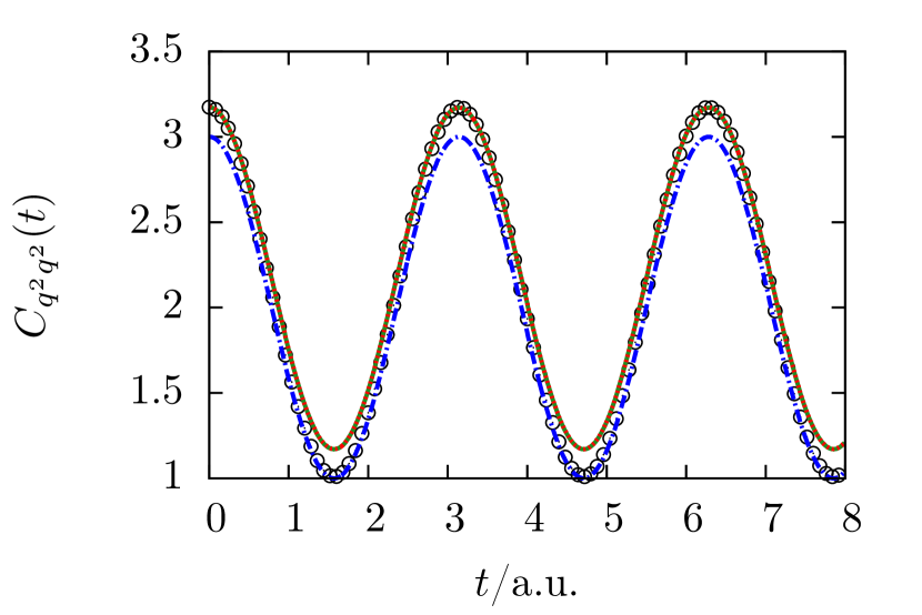
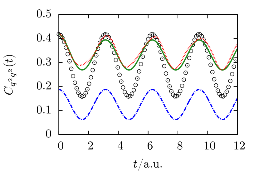
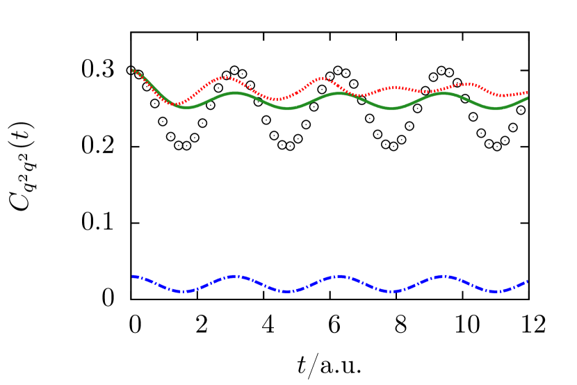
Figure 1: Position-squared autocorrelation function for a harmonic oscillator, with $\beta=1$ (top), $\beta=4$ (middle) and $\beta=10$ (bottom). Black circles, quantum; solid green line, TRPMD (with optimal damping); red dots, RPMD; blue dot-dashes, CMD.

CMD, RPMD and TRPMD correlation functions and spectra have already been the subject of many numerical studies kin98 ; hab13 ; vot96 ; ros14 ; ros14com ; hel15trpmd ; kre13 ; men11 ; wit09 ; iva10 ; hab09 ; sul11 ; sul14 whose results have been broadly summarized in the introduction. To clarify the nature of the approximations inherent in CMD, RPMD and TRPMD from Matsubara dynamics, we examine the position-squared autocorrelation function for a harmonic oscillator, for which Matsubara dynamics is exactly equal to the quantum result but both RPMD and CMD fail to qualitatively reproduce hor05 . CMD produces the incorrect result at $t=0$ but then oscillates at the correct frequency (though incorrect amplitude), whereas RPMD is exact at zero time but then deviates wildly from the quantum result at finite time due to the presence of the spurious frequencies in the higher normal modes hor05 ; jan14 . The “nonlinear operator” problem for which this is the archetypal model not only occurs in toy systems but is also observed in inelastic neutron scattering cra06 ; hab13 .

The exact quantum position-squared autocorrelation function in the harmonic potential Eq. (18) is hor05 ; jan14

$$c_{q^{2}q^{2}}(t)=\frac{\hbar^{2}}{4m^{2}\omega_{h}^{2}}\Bigg{[} \frac{2}{\beta\hbar\omega_{h}}\coth\left(\frac{\beta\hbar\omega_{h}}{2}\right)\cos(2\omega_{h}t)$$

$$+2\coth^{2}\left(\frac{\beta\hbar\omega_{h}}{2}\right)-1\Bigg{]}.$$ (23)

which in appendix B we show is exactly replicated by the Matsubara correlation function. For RPMD, it is hor05 ; jan14

$$C_{q^{2}q^{2}}^{\rm RPMD}(t)=\frac{1}{\beta^{2}m^{2}}\sum_{j=-(M-1)/2}^{(M-1)/2}\frac{1}{\omega_{h}^{2}+\tilde{\omega}_{j}^{2}}\left\{\frac{2\cos^{2}[(\omega_{h}^{2}+\tilde{\omega}_{j}^{2})^{1/2}t]}{\omega_{h}^{2}+\tilde{\omega}_{j}^{2}}+\sum_{k=-(M-1)/2}^{(M-1)/2}\frac{1}{\omega_{h}^{2}+\tilde{\omega}_{k}^{2}}\right\}$$ (24)

whereas the TRPMD result for the optimal damping frequencies $\Gamma_{jj^{\prime}}=2|\tilde{\omega}_{j}|\delta_{jj^{\prime}}$ is

$$C_{q^{2}q^{2}}^{\rm TRPMD}(t)= \frac{1}{\beta^{2}m^{2}}\sum_{j=-(M-1)/2}^{(M-1)/2}\frac{1}{\omega_{h}^{2}+\tilde{\omega}_{j}^{2}}\Bigg{\{}\frac{2e^{-2|\tilde{\omega}_{j}|t}}{\omega_{h}^{2}+\tilde{\omega}_{j}^{2}}\left[\cos(\omega_{h}t)+\frac{\tilde{\omega}_{j}}{\omega_{h}}\sin(\omega_{h}t)\right]^{2}+\sum_{k=-(M-1)/2}^{(M-1)/2}\frac{1}{\omega_{h}^{2}+\tilde{\omega}_{k}^{2}}\Bigg{\}}.$$ (25)

For comparison, the CMD position-squared autocorrelation function (using the CMD with classical operators method hor05 ; vot96 ; ros14 ; kin98 ) is

$$C_{q^{2}q^{2}}^{\rm CMD}(t)=\frac{1}{(\beta m\omega_{h}^{2})^{2}}\left[2\cos(\omega_{h}t)^{2}+1\right].$$ (26)

We use parameters to facilitate comparison with previous literature hor05 ; $\hbar=k_{\rm B}=m=\omega_{h}=1$ and results for systems of varying $\beta$ are presented in Fig. 1.

At high temperatures ($\beta=1$), all methods are a good approximation to the quantum result and the RPMD and TRPMD results are indistinguishable to within graphical accuracy. At $\beta=4$, the amplitude of oscillations is incorrect for all methods, though TRPMD starts at the correct value whereas CMD is too low. The RPMD correlation function shows deviations from harmonic behaviour due to the higher normal modes. At $\beta=10$, the CMD correlation function is far too small and RPMD cannot replicate the oscillations, unlike TRPMD.

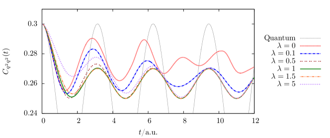
Figure 2: Position-squared autocorrelation function for a harmonic oscillator at $\beta=10$, showing the exact quantum result and TRPMD at a varying friction parameters. For clarity, the figure is zoomed in around the TRPMD correlation function.

We then examine the effect of different friction parameters in Fig. 2, choosing the $\beta=10$ system to exemplify the effect of damping. The $\lambda=0$ (RPMD) result oscillates erratically, as in the third panel of Fig. 1. Applying very small friction ($\lambda=0.1$) noticeably improves the correlation function but contamination from higher normal modes is still evident. Around the optimal damping ($\lambda=0.5$, $\lambda=1$ and $\lambda=1.5$) the correlation functions are extremely similar, settling to the correct frequency (though incorrect amplitude) after one oscillation. Increasing the friction yet further ($\lambda=5$) causes the correct oscillation frequency (as all modes apart from the centroid are overdamped) but the slow decay of the heavily overdamped higher normal modes causes midpoint of the oscillation to decay slowly over time. These results (which can be derived analytically for the harmonic oscillator) are broadly consistent with those observed numerically in more complex systems (see Fig. 3 of Ref. ros14, ), where a broad range of friction parameters around $0.5\leq\lambda\leq 1.5$ led to similar results.

For the position-squared autocorrelation function at least, it seems that TRPMD with $\lambda=1$ combines the best features of both RPMD and CMD; the correct zero-time value and the correct amplitude of oscillation, and that there exists a sizeable range of friction parameters around $\lambda=1$ in which these qualitative features are captured. However, TRPMD with optimal friction is by no means perfect; the amplitude of oscillations decays within one oscillation and is far too small, since by this time all modes apart from the centroid are essentially completely damped.

IV.3 Parabolic barrier

For an unbound, scattering system, or where barrier dynamics are required such as thermal rate calculation, we instead consider a parabolic barrier with a potential

$$V(q)=-\tfrac{1}{2}m\omega_{b}^{2}.$$ (27)

We firstly observe that RPMD (and CMD) have qualitatively incorrect fluctuation dynamics at barriers; hel15rel while all the Matsubara modes are scattering,

$$Q_{j}(t)= Q_{j}\cosh(\omega_{b}t)+\frac{\bar{P}_{j}}{m\omega_{b}}\sinh(\omega_{b}t)$$

$$+i\frac{\tilde{\omega}_{j}}{\omega}Q_{-j}\sinh(\omega_{b}t)$$ (28)

the RPMD higher normal modes are generally bound, with a frequency of $\bar{\omega}_{j}=\sqrt{\tilde{\omega}_{j}-\omega_{b}^{2}}$. As the temperature is lowered, modes become successively unbound, beginning with $j=\pm 1$ at the ‘crossover’ temperature ric09 ; hel13

$$\beta_{c}=\frac{2\pi}{\hbar\omega_{b}}$$ (29)

and the $j$th normal mode will become unbound when $\beta>|j|\beta_{c}$, but with a scattering (imaginary) frequency of $\sqrt{\omega_{b}-\tilde{\omega}_{j}^{2}}$. Despite these shortcomings, RPMD has been very accurate for rate calculation, partly because of the correct short-time TST limit hel15rel (see Introduction), and since reaction above the crossover temperature is dominated by the motion of the centroid, which scatters at the correct imaginary frequency in RPMD, TRPMD and CMD.

Considering the $j$th mode at a temperature $\beta<|j|\beta_{c}$ such that it is bound in RPMD ($\omega_{b}<|\tilde{\omega}_{j}|$), very weak friction ($\Gamma_{jj}/2<\tilde{\omega}_{j}^{2}-\omega_{b}^{2}$) leads to damped oscillatory motion as in Eq. (20), but with $\acute{\omega}_{j}=\sqrt{-\omega_{b}^{2}+\tilde{\omega}_{j}^{2}-\Gamma_{jj}^{2}/4}$. Stronger friction leads to an overdamping solution,

$$\mathcal{Q}_{j}(t)=e^{-\Gamma_{jj}t/2}\Bigg{[} Q_{j}\cosh(\zeta_{j}t)$$

$$+\left(\frac{P_{j}}{m\zeta_{j}}+\frac{Q_{j}\Gamma_{jj}}{2\zeta_{j}}\right)\sinh(\zeta_{j}t)\Bigg{]}$$ (30)

where $\zeta_{j}=\sqrt{\omega_{b}^{2}-\tilde{\omega}_{j}^{2}+(\Gamma_{jj}/2)^{2}}$ can be considered the imaginary frequency counterpart to $\acute{\omega}_{j}$.

The presence of the $e^{-\Gamma_{jj}t/2}$ prefactor in Eq. (30), which in the oscillatory case of Eq. (20) causes damping but leaves the frequency untouched, means that no physical (i.e. real and positive mac08 ) value of the friction parameter exists which would make Eq. (30) have an unbound solution. Increasing friction merely causes the oscillator to become more overdamped.

If the normal mode is unbound in RPMD ($\beta>|j|\beta_{c}$ and therefore $\omega_{b}>|\tilde{\omega}_{j}|$) then Eq. (30) still holds, but the solution has a scattering component for all $\Gamma_{jj}$ since $-\Gamma_{jj}/2+\zeta_{j}>0$. We would like to increase the escape rate from the RPMD value of $\sqrt{\omega_{b}^{2}-\tilde{\omega}_{j}^{2}}$ to $\omega_{b}$, but adding friction only decreases the rate of escape from the barrier, as can be observed from the vanishing escape rate at high friction,

$$\lim_{\Gamma_{jj}\to\infty}-\Gamma_{jj}/2+\zeta_{j}=2\frac{\omega_{b}^{2}-\omega_{j}^{2}}{\Gamma_{jj}}.$$ (31)

In order for the largest positive unbound solution (the highest root of the characteristic equation whose solution gives Eq. (30)) to be the physical barrier frequency, the friction would have to be negative; $\Gamma_{jj}=-\tilde{\omega}_{j}^{2}/\omega_{b}$.

For the (artificial) case of a reaction whose reaction co-ordinate is solely a single non-centroid normal mode, the above result is corroborated by Kramers theory kra40 ; nit06 ; hel15trpmd which states that the transmission coefficient $\kappa(t)$ decreases with friction as

$$\lim_{t\to\infty}\kappa(t)\simeq\sqrt{1+\alpha^{2}}-\alpha$$ (32)

where $\alpha=\Gamma_{jj}/2\bar{\omega}_{j}$ and $\bar{\omega}_{j}$ is the barrier frequency in ring-polymer space defined above. However, the transmission coefficient across a parabolic barrier is unity in Matsubara dynamics, and adding friction in TRPMD will only decrease this. Consequently, application of friction to RPMD will not ameliorate the qualitative problems with the RPMD higher normal modes at a barrier, and in some cases will worsen them.

V Discussion

The friction matrix $\Gamma_{jj^{\prime}}=2|\tilde{\omega}_{j}|\delta_{jj^{\prime}}$ obtained section IV.1 corresponds to critical damping of the ring polymer springs in the absence of an external potential, but not critical damping of the ring polymer modes in a harmonic oscillator (where the external frequency must also be considered), and can be determined without knowledge of the frequencies present in the external potential. Obviously, chemical systems will not be purely harmonic but in many systems (such as vibrating bond) this will be a reasonable approximation.

Previous literature has explored a range of scaled friction matrices of $\lambda\bm{\Gamma}$ and found $\lambda=1/2$ to be optimal for some spectra, justifying this on the grounds of optimal sampling of the harmonic ring polymer potential energy ros14 , but also finding there to be a wide range of $\lambda$ close to $\lambda=1/2$ in which results are broadly similar (as also seen in Fig. 2). We suspect that a numerically favourable value of $\lambda=1/2$ is due to interplay between shifting the frequencies of the higher normal modes to the external frequency (implying $\lambda=1$), moving the maximum in the spectral peak (implying $\lambda=2^{-1/2}$), and avoiding harsh damping which would decorrelate the modes too quickly to capture their dynamics and broaden spectral peaks ros14com (implying the weakest possible friction which removes spurious resonances). We can certainly find no reason to use $\lambda>1$.

This definition of the friction matrix means that $\Gamma_{00}=0$ (for all $\lambda$) meaning that the centroid is unthermostatted, so all the results which have previously been derived for TRPMD, such as its short-time error compared to the quantum result ros14 , still hold. A new result is that TRPMD, like RPMD, will have the exact Matsubara force on the centroid, since the error term does not act upon the centroid. Like RPMD and CMD but not LSC-IVR, the TRPMD dynamics will also satisfy detailed balance hel15trpmd , and the error scaling in the higher normal modes in time will be the same as that for RPMD, namely $i\mathcal{L}_{\Im}^{[M]}-\mathcal{A}_{\rm wn}^{[M]{\dagger}}\propto 1/\beta\hbar$.

This choice of friction matrix also means that the TRPMD correlation function of a linear operator will deviate from the Matsubara correlation due to higher-order coupling between the centroid dynamics and the damping (and random kicks) of the higher normal modes via anharmonicity in the potential. This causes slight broadening of spectral lines (a far smaller issue than the curvature problem of CMD or the spurious resonances of RPMD) ros14 , but the extra friction noticeably slows reaction rates beneath the crossover temperature hel15trpmd where the unbound and thermostatted higher normal modes are part of the optimal dividing surface ric09 . For nonlinear operators, TRPMD (like RPMD) would be expected to break down faster than for linear operators due to the error term only acting directly on the higher normal modes, though the example of the position-squared autocorrelation function given above suggests that with a careful choice of friction the breakdown may not be too drastic.

Although the analysis for a parabolic barrier in section IV.3 does not suggest that the TRPMD rate will ever be closer to the Matsubara (and therefore quantum) rate, TRPMD could be computationally advisable above the crossover temperature (where passage over the barrier is dominated by motion of the unthermostatted centroid) since the TRPMD trajectories may sample the path-integral phase space more efficiently than the RPMD trajectories hel15trpmd , and same may be true for other observable properties which are dominated by barrier crossing, such as diffusion ros14 . The TRPMD time-evolution is also simpler computationally since the same dynamics can be used for thermostatting and computation of the correlation function ros14 . Nevertheless, these results suggest that beneath the crossover temperature, TRPMD is not to be advised for reaction rates, a result broadly supported by numerical tests in one-dimensional and multidimensional gas-phase systems hel15trpmd .

All the results presented here generalize immediately to multidimensional systems, where the friction is applied in $F(N-1)$ normal modes and springs exist between $N$ replicas of the physical system. For nonlinear operators one cannot, in general, easily relate the Kubo and Generalized Kubo forms [Eqs. (1) and (2)] (the position-squared operator explored above being an exception). For reaction rates involving the highly nonlinear flux and side operators this is resolved by relating the generalized Kubo form to the exact quantum expression when there is no recrossing of the path-integral dividing surface (and those orthogonal to it in path-integral space) by the exact quantum dynamics of the system hel13 ; alt13 ; hel13unique , such that TRPMD rate theory will give the exact quantum rate in the absence of recrossing by either the TRPMD dynamics or exact quantum dynamics. hel15trpmd

VI Conclusions

In this article we have shown, for the first time, how to obtain thermostatted ring polymer molecular dynamics (TRPMD) from exact quantum dynamics by a series of approximations, each with an analytic error term. We firstly discard fluctuations of the highest $N-M$ normal modes from the exact quantum time evolution, giving Matsubara dynamics hel15 . To derive a computationally tractable approximation to Matsubara dynamics, we perform a contour integral in the momenta (where we assume the edge terms to be zero), giving a correlation function with the (real) ring polymer distribution, but whose Liouvillian is complex. We then replace the imaginary part of the complex Liouvillian with a white-noise Fokker-Planck term, giving TRPMD.

Each of these approximations has its limitations and benefits. The primary consequence of discarding the fluctuations of the highest normal modes from the exact quantum dynamics (leading to Matsubara dynamics) is neglect of interference effects and mixing of quantum states. In physical systems this is seen as the failure of TRPMD to replicate the Fermi resonance in the Zundel cation ros14 (CMD and RPMD also fail here ros14 , as would be expected as they too are approximations to Matsubara dynamics hel15rel ). However, discarding these fluctuations leads to a classical-like dynamics which preserves the quantum Boltzmann distribution. hel15

We then show that a careful choice of the friction matrix (which is system independent and known in advance) will cause all ring polymer normal modes to oscillate at the correct frequency in a harmonic potential, and therefore will reproduce the correct frequency of oscillation of the position-squared autocorrelation function and the correct $t=0$ value; neither CMD nor RPMD will replicate both of these properties. However, the oscillations’ amplitude is too small, and we suspect that a generalized Langevin equation cer10 ; nit06 may be more successful than a simple white noise thermostat, in that it may be constructed to produce the correct frequency of oscillation of the higher normal modes but with smaller damping (and maybe even the correct maxima in the position and momentum autocorrelation spectra). The same analysis, but for a parabolic barrier, shows that no physical friction parameter will solve the qualitative innacurracies in the higher ring polymer normal mode fluctuations. Usage of unphysical negative friction mac08 ; che02 as a possible solution to this problem is left as further work. Future research could also include extension to non-adiabatic systems where RPMD has been successful. hel11 ; ana13 ; ana10 ; men14 ; ric13 ; ric14 ; men11 ; kre13

In closing, the results presented here give an a priori prescription for when to use TRPMD: it should be used for computation of spectra and other properties of bound systems where the correct oscillation frequencies are required, and avoided for rate calculation beneath the crossover temperature.

Appendix A Matsubara modes

The ring-polymer normal modes are defined as

$$Q_{j}=\sum_{i=0}^{N-1}\frac{T_{ij}}{\sqrt{N}}q_{i}$$ (33)

where $j=-N/2+1,\ldots,0,\ldots,N/2$ and likewise for ${\bf P}$, where

$$T_{ij}=\left\{\begin{array}[]{ll}N^{-1/2}&j=0\\ \sqrt{2/N}\sin(2\pi ij/N)&1\leq j\leq N/2-1\\ N^{-1/2}(-1)^{i}&j=N/2\\ \sqrt{2/N}\cos(2\pi ij/N)&-N/2+1\leq j\leq-1\end{array}\right.$$ (38)

where the $j=N/2$ mode is omitted if $N$ is odd. The transformation is not unitary, but defined such that the normal modes converge in the $N\to\infty$ limit. This leads to frequencies in the complex Boltzmann distribution of

$$\omega_{j}=\frac{2\sin(j\pi/N)}{\beta_{N}\hbar}$$ (39)

which, for large $N$ and finite $j$, become the Matsubara frequencies mat55

$$\tilde{\omega}_{j}=\lim_{N\to\infty}\omega_{j}=\frac{2\pi j}{\beta\hbar}.$$ (40)

The observables $A({\bf Q})$ and $B({\bf Q})$ are obtained by making by substituting

$$q_{i}=\sum_{j=-(M-1)/2}^{(M-1)/2}T_{ij}\sqrt{N}Q_{j}$$ (41)

into $A({\bf q})$ and $B({\bf q})$ respectively, which also leads to a ‘Matsubara potential’,

$$U^{[M]}({\bf Q})=\frac{1}{N}\sum_{i=0}^{N-1}V\!\left(\sum_{j=-(M-1)/2}^{(M-1)/2}T_{ij}\sqrt{N}Q_{j}\right).$$ (42)

Appendix B Equivalence of quantum and Matsubara correlation functions

To show that the Matsubara correlation function is equivalent to Eq. (23), we firstly calculate the Matsubara correlation function using the harmonic analysis in the supplementary material of Ref. hel15rel, , giving

$$C_{q^{2}q^{2}}^{[N]}(t)= \frac{1}{\beta^{2}m^{2}\omega_{h}^{4}}\Bigg{[}\cos(2\omega_{h}t)\sum_{j=-(M-1)/2}^{(M-1)/2}\frac{1}{1+(\tilde{\omega}_{j}/\omega_{h})^{2}}+\sum_{j=-(M-1)/2}^{(M-1)/2}\frac{1-(\tilde{\omega}_{j}/\omega_{h})^{2}}{(1+(\tilde{\omega}_{j}^{2}/\omega_{h}))^{2}}$$

$$+\sum_{j=-(M-1)/2}^{(M-1)/2}\sum_{k=-(M-1)/2}^{(M-1)/2}\frac{1}{1+(\tilde{\omega}_{j}/\omega_{h})^{2}}\frac{1}{1+(\tilde{\omega}_{k}/\omega_{h})^{2}}\Bigg{]}$$ (43)

The Matsubara frequency summation alt10 is performed by examining the integral

$$\oint dz\frac{\cot(z)}{z^{2}+x^{2}}$$ (44)

around a circle of infinite radius, origin zero, we find

$$x\coth(x)=\lim_{M\to\infty}\sum_{j=-(M-1)/2}^{(M-1)/2}\frac{1}{1+(j\pi/x)^{2}}$$ (45)

and by differentiation of Eq. (45), that

$$x^{2}[\coth^{2}(x)-1]= \lim_{M\to\infty}\sum_{j=-(M-1)/2}^{(M-1)/2}\frac{1-(j\pi/x)^{2}}{(1+(j\pi/x)^{2})^{2}}.$$ (46)

Subsituting $x=\beta\hbar\omega_{h}/2$ into Eq. (45) and Eq. (46), and these expressions into Eq. (43) gives Eq. (23) as required.

Appendix C Analyticity in the complex plane

Consider an observable $B({\bf P},{\bf Q},t)$, which is propagated by the Liouvillian

$$\mathcal{L}=\left(\nabla_{\bf P}H\right)\cdot\nabla_{\bf Q}-\left(\nabla_{\bf Q}H\right)\cdot\nabla_{\bf P}$$ (47)

where $H$ is the Hamiltonian of the system and an analytic, but not necessarily real, function of ${\bf P}$ and ${\bf Q}$. The propagation is formally

$$\frac{d}{dt}B({\bf P},{\bf Q},t)= \mathcal{L}B({\bf P},{\bf Q},t)$$ (48)

$$B({\bf P},{\bf Q},t)= e^{\mathcal{L}t}B({\bf P},{\bf Q},0)$$ (49)

This (obviously) requires $B({\bf P},{\bf Q},t)$ to be single valued, and the exponentiated expression Eq. (49) to exist. If $B({\bf P},{\bf Q},t)$ is an analytic function for all values of ${\bf z}$, then (by the Cauchy-Riemann relations)

$$\frac{\partial}{\partial P_{j}^{*}}B({\bf P},{\bf Q},t)=0\ \forall j$$ (50)

where $P_{j}^{*}$ is the complex conjugate of $P_{j}$ (and likewise for $Q_{j}^{*}$). If $H$ is analytic then

$$\frac{\partial}{\partial P_{j}^{*}}H=0\ \forall j$$ (51)

which means that (using $H$ being continuous, Schwarz’ theorem and therefore $\frac{\partial}{\partial P_{j}^{*}}\frac{\partial}{\partial P_{j}}=\frac{\partial}{\partial P_{j}}\frac{\partial}{\partial P_{j}^{*}}$) the commutation relations exist

$$\frac{\partial}{\partial P_{j}^{*}}\mathcal{L}= \mathcal{L}\frac{\partial}{\partial P_{j}^{*}}$$ (52)

Using the definition of an exponential as its power expansion we then see,

$$\frac{\partial}{\partial P_{j}^{*}}B({\bf P},{\bf Q},t)= \frac{\partial}{\partial P_{j}^{*}}e^{\mathcal{L}t}B({\bf P},{\bf Q},0)$$ (53)

$$= e^{\mathcal{L}t}\frac{\partial}{\partial P_{j}^{*}}B({\bf P},{\bf Q},0)$$ (54)

$$= 0$$ (55)

so $B({\bf P},{\bf Q},t)$ remains an analytic function of $P_{j}$ for all time (and likewise for $Q_{j}$). This is true $\forall j$ (and $\forall t$), and by Hartog’s Theorem, true for $B({\bf P},{\bf Q},t)$ everywhere. This means that $B({\bf P},{\bf Q},t)$ obeys the Cauchy Riemann relations and can have no poles in the complex plane. The Boltzmann distribution is also holomorphic, and provided that the zero-time observable $A({\bf P},{\bf Q},0)$ is also holomorphic (which almost all physical observables are) the entire integrand of Eq. (4) will be.

We then complete the square in the complex Matsubara distribution, giving Eq. (4) where the edges of the rectangle used in the contour integration are

$$\mathcal{E}(t)= \lim_{\bm{\pi}\to\infty}\int d{\bf Q}\left[\prod_{j=-(M-1)/2}^{(M-1)/2}i\int_{0}^{m\omega_{j}Q_{-j}}d\Pi_{j}\right]$$

$$\qquad\times e^{-\beta[H(\bm{\pi}+i\bm{\Pi},{\bf Q})-i\theta(\bm{\pi}+i\bm{\Pi},{\bf Q})]}A({\bf Q})e^{\mathcal{L}^{[M]}_{\bm{\pi}+i\bm{\Pi}}t}B({\bf Q})$$

$$+\lim_{\bm{\pi}\to-\infty}\int d{\bf Q}\left[\prod_{j=-(M-1)/2}^{(M-1)/2}i\int_{0}^{m\omega_{j}Q_{-j}}d\Pi_{j}\right]$$

$$\qquad\times e^{-\beta[H(\bm{\pi}+i\bm{\Pi},{\bf Q})-i\theta(\bm{\pi}+i\bm{\Pi},{\bf Q})]}A({\bf Q})e^{\mathcal{L}^{[M]}_{\bm{\pi}+i\bm{\Pi}}t}B({\bf Q})$$ (56)

where $\pi_{j}=\Re P_{j}$, $\Pi_{j}=\Im P_{j}$, and $\mathcal{L}^{[M]}_{\bm{\pi}+i\bm{\Pi}}$ is the Matsubara Liouvillian Eq. (7) continued into the complex plane.

The edge terms can be proven to be zero in a number of limits. Specifically, for $A({\bf Q})$ and $B({\bf Q})$ which are at most exponential in ${\bf P}$ and/or ${\bf Q}$, the edge terms will vanish when the trajectories are real ($\bm{\Pi}=0$) where conservation of energy arguments can be used in a bound system and in a scattering system whose potential tends to a constant value far out. The edges will also be zero in any system at $t=0$ where the momentum integral can be evaluated analytically, and where discarding $\mathcal{L}^{[M]}_{\Im}$ (and thereby keeping the trajectories real) is no approximation, namely up to $\mathcal{O}(t^{2})$ for nonlinear operators and $O(t^{6})$ for linear operators hel15rel ; ros14 .

For systems where the trajectories are known analytically, such as a free particle, parabolic well and barrier, even though $\bm{\pi}(t)\to\infty$ as $\bm{\pi}(0)\to\infty$, careful consideration of the limits and application of l’Hôpital’s rule shows that the edge term still vanishes.

Despite the above promising results, trajectories in the complex plane are frequently not bounded ben08 and in general it is difficult to determine whether or not terms of the form in Eq. (56) will converge aar10trust for any general potential. A proof of whether $\mathcal{E}(t)$ can be neglected in any general case is left as further work.

Appendix D TRPMD position-squared correlation functions

The correlation function can be evaluated by considering each normal mode separately and deriving the correlation function for a single harmonic oscillator cer10phd ; nit06 ; gar09 . For $0\leq\lambda\leq 1$, the correlation function is

$$C_{q^{2}q^{2}}^{[N]}(t)=\frac{1}{\beta^{2}m^{2}}\sum_{j=-(M-1)/2}^{(M-1)/2}\frac{1}{\omega_{h}^{2}+\tilde{\omega}_{j}^{2}}\left\{\frac{2e^{-\Gamma_{jj}t}}{\omega_{h}^{2}+\tilde{\omega}_{j}^{2}}\left[\cos(\acute{\omega}_{j}t)+\frac{\gamma_{j}}{2\acute{\omega}_{j}}\sin(\acute{\omega}_{j}t)\right]^{2}+\sum_{k=-(M-1)/2}^{(M-1)/2}\frac{1}{\omega_{h}^{2}+\tilde{\omega}_{k}^{2}}\right\}$$ (57)

with $\acute{\omega}_{j}$ defined in Eq. (21). If $\lambda>1$, we define

$$j_{\rm cut}=\left\lfloor\frac{\beta\hbar\omega_{h}}{2\pi\sqrt{\lambda^{2}-1}}\right\rfloor$$ (58)

where $\lfloor\cdot\rfloor$ is the floor function, so all modes with $|j|>j_{\rm cut}$ will be overdamped. The correlation function is

$$C_{q^{2}q^{2}}^{[N]}(t)= \frac{1}{\beta^{2}m^{2}}\sum_{j=-j_{\rm cut}}^{j_{\rm cut}}\frac{1}{\omega_{h}^{2}+\tilde{\omega}_{j}^{2}}\Bigg{\{}\frac{e^{-\Gamma_{jj}t}}{\omega_{h}^{2}+\tilde{\omega}_{j}^{2}}\left[1+\frac{\Gamma_{jj}^{2}}{4\zeta_{j}^{2}}+\left(1-\frac{\Gamma_{jj}^{2}}{4\zeta_{j}^{2}}\right)\cos(2\zeta_{j}t)+\frac{\Gamma_{jj}}{\zeta_{j}}\sin(2\zeta_{j}t)\right]+\sum_{k=-(M-1)/2}^{(M-1)/2}\frac{1}{\omega_{h}^{2}+\tilde{\omega}_{k}^{2}}\Bigg{\}}$$

$$+\frac{2}{\beta^{2}m^{2}}\sum_{j=j_{\rm cut}+1}^{M/2-1}\frac{1}{\omega_{h}^{2}+\tilde{\omega}_{j}^{2}}\Bigg{\{}\frac{e^{-\Gamma_{jj}t}}{\omega_{h}^{2}+\tilde{\omega}_{j}^{2}}\left[1-\frac{\Gamma_{jj}^{2}}{4\zeta_{j}^{2}}+\left(1+\frac{\Gamma_{jj}^{2}}{4\zeta_{j}^{2}}\right)\cosh(2\zeta_{j}t)+\frac{\Gamma_{jj}}{\zeta_{j}}\sinh(2\zeta_{j}t)\right]+\sum_{k=-(M-1)/2}^{(M-1)/2}\frac{1}{\omega_{h}^{2}+\tilde{\omega}_{k}^{2}}\Bigg{\}}$$ (59)

where we have noted that contributions from modes $j$ and $-j$ are the same. If a mode is critically damped then the term in square brackets for that mode becomes $2+\Gamma_{jj}^{2}t^{2}/2+2\Gamma_{jj}t$.

References

- (1) C. Gardiner, Stochastic Methods (Springer, Berlin, 2009).
- (2) R. Zwanzig, Nonequilibrium statistical mechanics (Oxford University Press, New York, 2001).
- (3) S. Habershon, D.E. Manolopoulos, T.E. Markland and T.F. Miller, Annu. Rev. Phys. Chem. 64 (1), 387 (2013).
- (4) J. Liu, Int. J. Quantum Chem. pp. n/a–n/a (2015).
- (5) W.H. Miller, PNAS 102 (19), 6660 (2005).
- (6) S. Habershon and D.E. Manolopoulos, J. Chem. Phys. 131 (24), 244518 (2009).
- (7) E. Wigner, Phys. Rev. 40, 749 (1932).
- (8) J. Liu and W.H. Miller, J. Chem. Phys. 126 (23), 234110 (2007).
- (9) Q. Shi and E. Geva, J. Chem. Phys. 118 (18), 8173 (2003).
- (10) J.E. Moyal, Math. Proc. Camb. Philos. Soc. 45, 99 (1949).
- (11) J. Cao and G.A. Voth, J. Chem. Phys. 100 (7), 5093 (1994).
- (12) J. Cao and G.A. Voth, J. Chem. Phys. 100 (7), 5106 (1994).
- (13) J. Cao and G.A. Voth, J. Chem. Phys. 101 (7), 6157 (1994).
- (14) J. Cao and G.A. Voth, J. Chem. Phys. 101 (7), 6168 (1994).
- (15) J. Cao and G.A. Voth, J. Chem. Phys. 101 (7), 6184 (1994).
- (16) G.A. Voth, Path-Integral Centroid Methods in Quantum Statistical Mechanics and Dynamics Adv. Chem. Phys. (, , 1996), pp. 135–218.
- (17) K. Kinugawa, Chemical Physics Letters 292 (4-6), 454 (1998).
- (18) D.R. Reichman, P.N. Roy, S. Jang and G.A. Voth, J. Chem. Phys. 113 (3), 919 (2000).
- (19) I.R. Craig and D.E. Manolopoulos, J. Chem. Phys. 121 (8), 3368 (2004).
- (20) I.R. Craig and D.E. Manolopoulos, J. Chem. Phys. 122 (8), 084106 (2005).
- (21) I.R. Craig and D.E. Manolopoulos, J. Chem. Phys. 123 (3), 034102 (2005).
- (22) M. Parrinello and A. Rahman, J. Chem. Phys. 80 (2), 860 (1984).
- (23) A. Witt, S.D. Ivanov, M. Shiga, H. Forbert and D. Marx, J. Chem. Phys. 130 (19), 194510 (2009).
- (24) S.D. Ivanov, A. Witt, M. Shiga and D. Marx, J. Chem. Phys. 132 (3), 031101 (2010).
- (25) M. Rossi, M. Ceriotti and D.E. Manolopoulos, J. Chem. Phys. 140 (23), 234116 (2014).
- (26) M. Ceriotti, Ph.D. thesis, ETH Zürich 2010.
- (27) A. Nitzan, Chemical Dynamics in Condensed Phases (Oxford University Press, New York, 2006).
- (28) G. Bussi and M. Parrinello, Phys. Rev. E 75, 056707 (2007).
- (29) M. Ceriotti, M. Parrinello, T.E. Markland and D.E. Manolopoulos, J. Chem. Phys. 133 (12), 124104 (2010).
- (30) M. Rossi, H. Liu, F. Paesani, J. Bowman and M. Ceriotti, J. Chem. Phys. 141 (18), 181101 (2014).
- (31) T.J.H. Hele and S.C. Althorpe, J. Chem. Phys. 138 (8), 084108 (2013).
- (32) S.C. Althorpe and T.J.H. Hele, J. Chem. Phys. 139 (8), 084115 (2013).
- (33) T.J.H. Hele and S.C. Althorpe, J. Chem. Phys. 139 (8), 084116 (2013).
- (34) T.J.H. Hele, Ph.D. thesis, University of Cambridge 2014.
- (35) T.J.H. Hele and Y.V. Suleimanov, J. Chem. Phys. (2015), (accepted).
- (36) T.J.H. Hele, M.J. Willatt, A. Muolo and S.C. Althorpe, J. Chem. Phys. 142 (13), 134103 (2015).
- (37) T.J.H. Hele, M.J. Willatt, A. Muolo and S.C. Althorpe, J. Chem. Phys. 142 (19), 191101 (2015).
- (38) A.R. Menzeleev, N. Ananth and T.F. Miller III, J. Chem. Phys. 135 (7), 074106 (2011).
- (39) R. Collepardo-Guevara, Y.V. Suleimanov and D.E. Manolopoulos, J. Chem. Phys. 130 (17), 174713 (2009).
- (40) R. Collepardo-Guevara, Y.V. Suleimanov and D.E. Manolopoulos, J. Chem. Phys. 133 (4), 049902 (2010).
- (41) Y.V. Suleimanov, R. Collepardo-Guevara and D.E. Manolopoulos, J. Chem. Phys. 134 (4), 044131 (2011).
- (42) A. Horikoshi and K. Kinugawa, J. Chem. Phys. 122 (17), 174104 (2005).
- (43) S. Jang, A.V. Sinitskiy and G.A. Voth, J. Chem. Phys. 140 (15), 154103 (2014).
- (44) Here we consider dynamics on a single Born-Oppenheimer potential energy surface and at temperatures sufficiently high that Bose-Einstein and Fermi-Dirac statistics need not be considered, which is the case for most systems to which CMD, RPMD and TRPMD have been applied.
- (45) R. Kubo, J. Phys. Soc. Jpn. 12 (6), 570 (1957).
- (46) J.O. Richardson and S.C. Althorpe, J. Chem. Phys. 131 (21), 214106 (2009).
- (47) H. Wang, X. Sun and W.H. Miller, J. Chem. Phys. 108 (23), 9726 (1998).
- (48) X. Sun, H. Wang and W.H. Miller, J. Chem. Phys. 109 (11), 4190 (1998).
- (49) T. Matsubara, Progress of Theoretical Physics 14 (4), 351 (1955).
- (50) C.M. Bender, D.C. Brody and D.W. Hook, Journal of Physics A: Mathematical and Theoretical 41 (35), 352003 (2008).
- (51) G. Aarts, E. Seiler and I.O. Stamatescu, Phys. Rev. D 81, 054508 (2010).
- (52) The higher normal modes are not explicitly represented in CMD, though are sometimes used as a computational device to construct the mean-field potentialhon06 .
- (53) Strictly speaking, this is TRPMD with Matsubara rather than ring-polymer frequencies, but will converge to conventional TRPMD in the limit of large hel15rel .
- (54) J.S. Kretchmer and T.F. Miller III, J. Chem. Phys. 138 (13), 134109 (2013).
- (55) Y.V. Suleimanov, W.J. Kong, H. Guo and W.H. Green, J. Chem. Phys. 141 (24), 244103 (2014).
- (56) I.R. Craig and D.E. Manolopoulos, Chem. Phys. 322 (1-2), 236 (2006), Real-time dynamics in complex quantum systems in honour of Phil Pechukas.
- (57) The RPMD and TRPMD correlation functions given here use the Matsubara frequencies , and converge to the conventional form using the ring-polymer frequencies in Eq. (39) in the large and large limit. The numerical results use the ring-polymer frequencies with , and their convergence with the same correlation function computed with Matsubara frequencies () was checked.
- (58) We note that there are many other approaches of varying mathematical complexity and accuracy for the computation of general correlation functions with CMDcao94_1 ; cao94_2 ; cao94_3 ; cao94 ; vot96 ; hor05 ; rei00 , and here restrict ourselves to methods which simply require direct computation of a correlation function.
- (59) J. MacFadyen, J. Wereszczynski and I. Andricioaei, J. Chem. Phys. 128 (11), 114112 (2008).
- (60) H. Kramers, Physica 7 (4), 284 (1940).
- (61) Rossi and Manolopoulos, private communication, (2015).
- (62) Michele Ceriotti, private communication, 2015.
- (63) L.Y. Chen, S.C. Ying and T. Ala-Nissila, Phys. Rev. E 65, 042101 (2002).
- (64) T.J.H. Hele, Master’s thesis, University of Oxford 2011.
- (65) N. Ananth, J. Chem. Phys. 139 (12), 124102 (2013).
- (66) N. Ananth and T.F. Miller, J. Chem. Phys. 133 (23), 234103 (2010).
- (67) A.R. Menzeleev, F. Bell and T.F. Miller, J. Chem. Phys. 140 (6), 064103 (2014).
- (68) J.O. Richardson and M. Thoss, J. Chem. Phys. 139 (3), 031102 (2013).
- (69) J.O. Richardson and M. Thoss, J. Chem. Phys. 141 (7), 074106 (2014).
- (70) For mathematical simplicity we consider odd here, even leads to the same result but with more algebrahel15 .
- (71) A. Altland and B. Simons, Condensed matter field theory (Cambridge University Press, New York, 2010 ; pp. 168–171), pp. 168–171.
- (72) T.D. Hone, P.J. Rossky and G.A. Voth, J. Chem. Phys. 124 (15), 154103 (2006).