Modelling solar low-lying cool loops with optically thick radiative losses.

Abstract

Aims. We investigate the increase of the DEM (differential emission measure) towards the chromosphere due to small and cool magnetic loops (height $\lesssim 8$ Mm, $T\lesssim 10^{5}$ K). In a previous paper we analysed the conditions of existence and stability of these loops through hydrodynamic simulations, focusing on their dependence on the details of the optically thin radiative loss function used.

Methods. In this paper, we extend those hydrodynamic simulations to verify if this class of loops exists and it is stable when using an optically thick radiative loss function. We study two cases: constant background heating and a heating depending on the density. The contribution to the transition region EUV output of these loops is also calculated and presented.

Results. We find that stable, quasi-static cool loops can be obtained by using an optically thick radiative loss function and a background heating depending on the density. The DEMs of these loops, however, fail to reproduce the observed DEM for temperatures between $4.6<\log T<4.8$. We also show the transient phase of a dynamic loop obtained by considering constant heating rate and find that its average DEM, interpreted as a set of evolving dynamic loops, reproduces quite well the observed DEM.

1 Introduction

The origin of the EUV output at temperatures below 1 MK is still widely debated in Solar Physics. The classical picture that the transition region (hereafter TR) emission originates from the base of the hot large-scale coronal loops strongly underestimates the observed EUV emission below 0.1 MK, but no alternative, quantitative view has gained consensus to-date. One of the proposed explanations hypothesizes that much of the TR plasma is confined in relatively small and cool magnetic loops (height $\lesssim 8$ Mm, $T\lesssim 10^{5}$ K), which are directly connected to the chromosphere but thermally insulated from the corona (Dowdy et al. 1986; Dowdy 1993; Feldman 1983; Feldman et al. 2001).

From an observational point of view, these loops are indeed very difficult to observe. The first, presumed direct observations present in the literature have been obtained with the VAULT instrument (Very High Angular Ultraviolet Telescope, Korendyke et al. 2001) in the H i Ly-$\alpha$ line. They show loop-like structures with estimated temperatures and densities ($T=10^{4}-3\times 10^{4}$ K, $P=0.1-0.3$ dyne cm^-2) that could be appropriate for the low-temperature end of cool loops (Patsourakos et al. 2007; Vourlidas et al. 2010). This interpretation has been debated by Judge & Centeno (2008). More recently, the launch of the IRIS spacecraft (De Pontieu et al. 2014), in June 2013, has given new possibilities to observe these loops. The analysis of the data obtained in spectral lines and continua covering a range of temperatures $\log T=3.7-7$ K with a spatial resolution of $\sim 0.4$”, represents a very good opportunity to look for structures with the dimension and temperatures of the class of loops described above. It is therefore not surprising that observations of highly dynamical cool, low-lying loops, in many respects similar to those we discuss in this paper, have recently been reported (Hansteen et al. 2014).

In a previous paper (Sasso et al. 2012, hereafter referred to as Paper I), we analyzed the general properties of quasi-static (velocity along the loop lower than 1 km/s) cool loops with $T\lesssim 0.1$ MK and their conditions of stability and existence under different and more realistic assumptions on the optically thin radiative loss function with respect to previous works (i.e., Cally & Robb 1991). In particular, we obtained through hydrodynamic simulations stable low-lying cool loops, even for a set of parameters that would prevent the formation of rigorously static loops. The existence of the loops we found is due indeed to small departures from static conditions, i.e. to the presence of a small but non-zero conductive flux and velocities, and to the requirement of nearly constant pressure (implying that our loops are limited to low heights above the chromosphere). In our simulations, we considered only the case of constant heating rate. We also showed that the emission of these cool loops, plus the emission of intermediate temperature loops ($0.1<T<1$ MK), can account for the observed radiative output below 1 MK.

From a theoretical point of view, there are still several points that need to be explored in order to determine the conditions under which cool loops could exist in the solar atmosphere. One important point is the shape of the radiative loss function below 0.1 MK, due to the presence of the H i Ly-$\alpha$ peak, which is very important for the existence of cool loops.

Our work is based on 1-D hydrodynamic simulations and aims at studying the conditions of existence of cool loops to understand, in particular, the mechanisms of their heating and energy balance through comparison between their simulated differential emission measure (hereafter, DEM) and the observed one. Peter et al. (2004, 2006) made the first successful attempt to reproduce the shape of the DEM curve quantitatively and qualitatively, even at temperatures below $\log T=5.3$ K. They synthesized spectra from three-dimensional MHD simulations of the whole Sun atmosphere, finding structures that could be related to the kind of loops we are studying. However, the cool loops we describe would be covered by only very few resolution elements in their simulation, and in any case resolving the gradients and the dynamics of the relevant quantities in our loop models would require a much higher resolution. Therefore, we regard our study as complementary to large-scale 3-D simulations.

As in Paper I, while looking for cool loops, we have also found low-lying quasi-static loops with temperatures in the range $1-5\times 10^{5}$ K. Following one of the latest loop classifications (Reale 2014), we should refer to these loops also as “cool coronal loops”. In order to avoid confusion, we will refer to them as “intermediate-temperature loops”.

In this paper we want to make a further step in the direction of considering more realistic assumptions for the simulations of cool loops with respect to Paper I, by introducing an optically thick radiative loss function. In Sec. 2, we describe the numerical model and introduce the radiative loss function adopted. In Sec. 3, we present the hydrodynamic simulations and the loops obtained (cool and intermediate-temperature loops) with different assumption on the heating rate and we discuss and analyze their properties. Section 3.4 is dedicated to the calculated DEMs of the loops obtained and to the comparison with the observed one. Finally, in the conclusions (Sec. 4), the role of the cool and intermediate-temperature loops in the solar atmosphere and the comparison with the observations is treated.

2 Numerical calculations

The set of hydrodynamic equations for mass, momentum, and plasma energy conservation for a fully ionized hydrogen plasma have been solved in a unidimensional, magnetically confined loop of constant cross-section with ARGOS, a 1-D hydrodynamic code with the fully adaptive-grid package PARAMESH (Antiochos et al. 1999; MacNeice et al. 2000). A fully adaptive-grid is necessary to adequately resolve one or more evolving regions of steep gradients. The hydrodynamic equations for mass, momentum, and energy, respectively, solved by ARGOS are

$$\frac{\partial}{\partial t}\rho+\frac{\partial}{\partial s}(\rho v) = 0,$$ (1)

$$\frac{\partial}{\partial t}(\rho v)+\frac{\partial}{\partial s}(P+\rho v^{2}) = -\rho g_{\parallel}(s),$$ (2)

$$\frac{\partial U}{\partial t}+\frac{\partial}{\partial s}\left(Uv+F_{\textmd{\tiny{c}}}\right) = -P\frac{\partial}{\partial s}v+E(s,t)-n^{2}\Lambda(T,P),$$ (3)

$$F_{\textmd{\tiny{c}}} = -10^{-6}T^{5/2}\frac{\partial}{\partial s}T.$$ (4)

where $t$ is the time, $\rho$ the mass density, $v$ the velocity, $P$, $T$ and $n$ are the gas pressure, temperature, and electron number density, respectively. $U$ is the internal energy, $s$ the curvilinear coordinate along the loop, $E(s,t)$ the assumed form for the input heating rate, $n^{2}\Lambda(T,P)$ the plasma radiative losses specified by the radiative loss function $\Lambda(T,P)$, $g_{\parallel}(s)$ the component of the solar gravity along the loop axis, and $F_{\textmd{\tiny{c}}}$ the thermal conductive flux, in CGS units.

The code is based on a loop geometry that assumes an arched loop of a given length $L$ and apex height above the chromosphere $h$ as described in Karpen et al. (2001); Spadaro et al. (2003). At each footpoint of the loop there is a thick chromosphere (26.7 Mm deep) acting as a mass reservoir, with temperature set to $T=9.5\times 10^{3}$ K. Since we take, by definition, the top of the chromosphere as the level at which the plasma drops below $9.5\times 10^{3}$ K, the exact position of the top of the chromosphere ($s=\pm L_{i}/2$ at the beginning of the simulation, $s$ being the curvilinear coordinate along the field lines) changes during the calculation with the plasma filling or evacuating the loop. So, at end of the simulation, we will have a new position for the top of the chromosphere $s=\pm L_{f}/2$ and, consequently, a new value of $h=h_{f}$ , where $h_{f}$ is no longer the geometrical parameter defining the shape of the loop, but the height of the loop apex above the $T=9.5\times 10^{3}$ K level.

The main input parameters for the calculations are the radiative loss function, the heating rate, the pressure (or the density) at the chromospheric reference temperature, and the loop geometry ($h$ and $L$). In Paper I, we used constant heating rates per unit volume throughout the loop. Following the more general approach of Antiochos & Noci (1986), we also consider the case of a constant heating rate per particle. The two cases are parametrized as follows:

$$E(s,t)=E_{\mathrm{h}}\>f(s)\>[n(s,t)/n_{\circ}]^{\gamma}\,,$$ (5)

where $\gamma=0$ is the case of constant heating per unit volume, and $\gamma=1$ corresponds to the case of constant heating per particle and $n_{\circ}=3.9882\times 10^{9}$ cm^-3 is the value of the density at the base of the loop, taken from the work of Kuin & Poland (1991). The function $f(s)$ specifies the variability of the heating rate (per particle or per volume) along the loop. With the exception of the discussion of Sec. 2.2, we will assume $f(s)=1$ throughout this paper. The radiative loss function adopted in this paper is described more in detail in the following section.

2.1 Radiative loss function

In order to estimate the radiative losses in the optically thick H Ly-$\alpha$ line, we used the calculations by Kuin & Poland (1991). Those authors computed the contribution to radiative losses of hydrogen and helium taking into account the effects of geometry and optical depths and the non-LTE (non-local thermodynamic equilibrium) ionization state of hydrogen and helium. They generated 3-D tables of radiative losses as a function of $T$, $P$ and slab thickness, for H and He. We combine those tables with the radiative losses of the other elements from the CHIANTI database (version 7.1, Landi et al. 2013) and the code interpolates these tables depending on the temperature and the pressure of the loop. We will refer to the resulting radiative loss function as $\Lambda_{\mathrm{kp}}$. We consider in the following calculations only the case of slab thickness equal to 200 km. This value is consistent with the dimensions of these loops as inferred from observations (Vourlidas et al. 2010; Hansteen et al. 2014).

There are other calculations of optically thick radiative losses in the literature, like the work of Carlsson & Leenaarts (2012) that is indeed more recent. This work is dedicated to the radiative cooling and heating only in the chromosphere, by combining detailed non-LTE radiative transfer calculations and time-dependent 2D MHD simulations. We decided to use the radiative losses calculated by Kuin & Poland (1991), even if older, because their results are presented in a form that can be easily incorporated in hydrodynamic flux-tube calculations and are expressly aimed at flux-tube modelling. In addition, their calculations are relevant to a broader temperature range more suitable for our calculations.

In Fig. 1 we show the radiative loss function $\Lambda_{\mathrm{kp}}$ plotted for different pressure values ($\log P$= -2, -1, 0, 3, red, yellow, green and blue line, respectively) and the one from the CHIANTI database, version 7.1 (Landi et al. 2013) (black line) from which we start to compute them. They are compared to some of the radiative loss functions used in Paper I, for which we obtained stable cool loops, that are: power-law segments function equal to $T^{2}$ for $\log T<4.95$ K and $T^{-1}$ for $\log T>4.95$ K (AN, dark grey line, Antiochos & Noci 1986); AN function plus a peak mimicking the H Ly-$\alpha$ losses (dark grey line plus diamond symbols); from the work of Dere et al. (2009) without the H contribution (light grey line). The black and the blue line represent the upper and the lower limit for the radiative loss functions: optically thin and optically thick case, respectively.

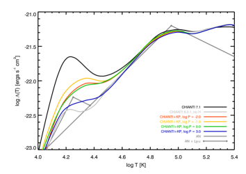
Figure 1: Radiative loss function $\Lambda_{\mathrm{kp}}$ plotted for different pressure values ($\log P$= -2, -1, 0, 3, red, yellow, green and blue line, respectively) and the one from the CHIANTI database, version 7.1 (Landi et al. 2013) (black line). Moreover, we plot some of the radiative loss functions used in Paper I: Antiochos & Noci (AN, dark grey line, 1986); AN function plus a peak mimicking the H Ly-$\alpha$ losses (dark grey line plus diamond symbols); from the CHIANTI database, version 6 (Dere et al. 2009), without the H contribution (light grey line).

2.2 Preliminary considerations on cool loop solutions

In their work, Antiochos & Noci (1986) turned their attention to the solutions of the hydrodynamic equations of loops with negligible conductive flux, and studied the properties and conditions of existence of their solutions under specific hypotheses about the radiative loss functions. They in particular approximated the optically thin function $\Lambda(T)$ with power-law segments: $\Lambda(T)\sim T^{a}$ for $T<0.1$ MK, and $\Lambda(T)\sim T^{-b}$ for $T>0.1$ MK, with $a$ and $b$ positive values. The conditions of existence and stability of such solutions were further and extensively studied by, e.g., Klimchuk et al. (1987); Cally & Robb (1991). Here we revisit some of those previous analyses, extending the results to consider the specific radiation losses functions we used in our simulations.

Antiochos & Noci (1986) solved the hydrodynamic equations Eq.1–3 assuming negligible conductive flux. The energy equation, Eq. 3, can then be rewritten as:

$$\left(\frac{P}{2kT}\right)^{2}\Lambda(T,P)=E(s,P)\;,$$ (6)

where now we considered the more general case of optically thick radiative loss function, $\Lambda(T,P)$, while $E(s,P)$ is given by Eq. 5.

It is convenient to define the following quantities:

$$H(T) \equiv 2kT/(m_{\mathrm{H}}\,g)\;,$$ (7)

$$\eta(s) \equiv g_{\parallel}(s)/g\;,$$ (8)

$$a(T,P) \equiv \partial\log\Lambda(T,P)/\partial\log T\;,$$ (9)

$$b(T,P) \equiv \partial\log\Lambda(T,P)/\partial\log P\;.$$ (10)

The quantity $a(T,P)$ can be interpreted as the local power-law index of the radiative loss function at a given temperature and pressure. The values of $a(T,P)$ for $\Lambda_{\mathrm{kp}}$ in the interval $\log T=$4.3–5 range from $\approx 0.5$ to $\approx 2$. The values for $b(T,P)$ are substantially smaller, ranging from $\approx-0.15$ to $\approx 0.2$ around the peak temperature of the Ly-$\alpha$ line.

Substituting Eq. 6 and Eq. 5 into the momentum equation, Eq. 2, with the above definitions the the equation for $T$ becomes:

$$\left[a(T,P)+\gamma-2\right]\frac{\mathrm{d}T}{\mathrm{d}s}=T\frac{1}{f(s)}\frac{\mathrm{d}f(s)}{\mathrm{d}s}+\left[b(T,P)+2-\gamma\right]\frac{T_{\circ}}{H(T_{\circ})}\eta(s)\;,$$ (11)

where $T_{\circ}$ is the temperature at the lower boundary of the loop.

The special case $a(T,P)=$ constant $=2-\gamma$ (power-law dependence of $\Lambda(T,P)$ with temperature, with exponent either 2 or 1, depending on the value of $\gamma$), reduces the above differential equation to the simpler expression:

$$H(T)=\left[-\frac{1}{f(s)}\frac{\mathrm{d}f(s)}{\mathrm{d}s}\right]^{-1}\left[b(T,P)+2-\gamma\right]\>\eta(s)\;.$$

In this case, any function $f(s)$ that is monotonically decreasing with height produces a loop solution, provided that $b(T,P)>-2+\gamma$ (true for $\Lambda_{\mathrm{kp}}$). The case $b=0$ and $a=2$ is the case we labelled “AN”, and is shown in Fig. 1 with a grey line.

In the remainder, we consider only the case $f(s)=1$; for simplicity, we further neglect the dependence of $\Lambda$ on pressure, i.e.: $b(T,P)=0$. In this case, Eq 11 can be integrated to obtain an implicit dependence of $T$ on $s$:

$$\theta(T,T_{\circ})=\frac{1}{H_{\circ}}\int_{s_{\circ}}^{s}\eta(\sigma)\>\mathrm{d}\sigma\;,$$ (12)

where the function $\theta(T,T_{\circ})$ is defined as:

$$\theta(T,T_{\circ})\equiv\left[\frac{\bar{a}(T,T_{\circ})+\gamma-2}{2-\gamma}\right]\left(\frac{T}{T_{\circ}}-1\right)\;,$$ (13)

while the quantity $\bar{a}(T,T_{\circ})$ is the “mean” power-law index:

$$\bar{a}(T,T_{\circ})\equiv\frac{1}{T-T_{\circ}}\int_{T_{\circ}}^{T}a(\tau)\>\mathrm{d}\tau\;.$$ (14)

The above equations highlights a first constraint for the existence of this kind of solutions: $\bar{a}(T,T_{\circ})>2-\gamma$. We have mentioned before that for the radiative loss function we are using, we have $a<2$ for $\log T>4.3$, it is clear that it would be very difficult to obtain cool solutions for the case of uniform heating per unit volume, $\gamma=0$.

The upper limit to the loop temperature as mapped by function $\theta(T,T_{\circ})$ is given by the maximum of $\int_{s_{\circ}}^{s}\eta(\sigma)\>\mathrm{d}\sigma/H_{\circ}$; in the case of a semicircular loop of radius $h$, this is $h/H_{\circ}$. However, a stronger constraint obviously follows from the consideration that $\int_{s_{\circ}}^{s}\eta(\sigma)\>\mathrm{d}\sigma$ is a monotonically increasing function, whereas $\theta(T,T_{\circ})$ is not, in general. Single-value solutions are therefore limited to the first local maximum of $\theta(T,T_{\circ})$, shown in Fig. 2 for the radiative loss function of Fig. 1 in the case $\gamma=0$ and $\gamma=1$.

The above simple considerations highlight one of the basic characteristics of cool loop solutions: their strong sensitivity on the details of the heating and of the radiation loss function.

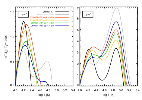
Figure 2: Function $\theta(T,T_{\circ})$ for the radiative loss functions shown in Fig. 1 in the case of $\gamma=0$ (left-hand panel) and $\gamma=1$ (right-hand panel).

3 Results and discussion

We ran numerous simulations, extensively exploring the parameter space, under different initial conditions. We consider a loop in a quasi-static equilibrium state when the plasma velocities are lower than 1–2 km/s. We took as an initial equilibrium state ($t=0$ s) for new simulations some of the cool loops obtained in Paper I, only changing the heating rate and the radiative loss function. The list of simulated loops, together with the relevant parameters, is given in Table 1 (cool loops) and Table 2 (intermediate temperature loops).

3.1 Loops from spatially uniform and temporally constant heating rate per unit volume

We start by making simulations with constant heating rate ($\gamma=0$) and using the radiative loss function $\Lambda_{\mathrm{kp}}$. As expected from the discussion in Sec. 2.2, we are not able to obtain stable cool loops since during the simulations, they become all hot ($T\sim 8\times 10^{5}$ K).

As an example, Fig. 3 shows the evolution of the mean temperature, density, and pressure of a loop (hereafter, Loop0) during a simulation started from a stable cool loop of top temperature $\sim 1.2\times 10^{4}$ K (Loop 24 of Table 1 in Paper I), assuming constant heating rate.

Loop0 stays for $\sim 42$ min in a cool state ($T<10^{5}$ K) even if not a stable one. The mean temperature of the loop oscillates between $1-2\times 10^{4}$ K (see left panel of Fig. 3) for $\sim 38$ min and then in $\sim 4$ min reaches much higher values. It becomes a quasi-static “coronal” loop, after $\sim 2.5$ h from the beginning of the simulation, reaching a top temperature of $\sim 8.5\times 10^{5}$ K. ARGOS gives the possibility to follow the evolution of the loop by storing the loop’s parameters at previously defined time steps. During the 4 minutes mentioned before, the simulation records three states characterized by maximum temperatures of $\sim 5,7$ and $9\times 10^{4}$ K, progressively. During the evolution of the loop, the maximum temperature is not always localized at $s=0$ (loop center) but also along the loop, i.e. at different values of $s$.

In Paper I, we obtained indeed quasi-static cool loops by using constant heating rate but the radiative loss functions used were different. From Fig. 1, it is clear that $\Lambda_{\mathrm{kp}}$ for pressure values characteristic of cool loops ($\log P\sim-2$) is higher than the losses used in Paper I and requires a higher thermal conductive flux from warmer regions to be balanced.

Figure 3: Evolution of the mean temperature, mean density, and mean pressure of Loop0, obtained from a simulation starting from a stable cool loop of top temperature $\sim 1.2\times 10^{4}$ K and constant heating rate per unit volume.

3.2 Loops from constant heating rate per particle

We perform new simulations with the radiative loss function $\Lambda_{\mathrm{kp}}$, and use constant heating rate per particle, setting $\gamma=1$ in Eq. 5. We list in Table 1 and discuss below a representative selection of cool loops in quasi-static equilibrium that we obtained in these conditions. All loops are obtained starting from four different loops of Paper I (Loops 17, 24, 26, and 27; the initial loop parameters are at the top of each loop group in Table 1), by changing the value of the constant $E_{\mathrm{h}}$ and the radiative loss function. We are able to obtain quasi-static cool loops with maximum temperature between $\sim 1.5$ and $6.2\times 10^{4}$ K, using $E_{\mathrm{h}}$ in the range $0.2-140\times 10^{-4}$ ergs cm^-3 s^-1. We are not able to obtain cool loops with maximum temperature in the range $4.3\lesssim\log T\lesssim 4.5$ K, since at those temperature, $a$, defined in eq. 9, becomes lower than 1 (see Sec. 2.2) due to the change of the slope of $\Lambda_{\mathrm{kp}}$. The cool loops found have the properties analytically predicted by Antiochos & Noci (1986): they are small ($L/2=7.5-8.8$ Mm and $h=1.67-3.05$ Mm), nearly isobaric, and in approximate balance between the heating rate and radiative losses. They have also the low-pressure values in the range predicted by Antiochos & Noci (1986), even if some loops have higher pressure (up to $\sim 7$ times) compared with the cool loops obtained in Paper I.

Table 1: Cool loop parameters at the end of the simulations when the loops have reached a quasi-static condition ($\gamma=1$). All loops are obtained starting from a loop of Paper I (the initial loop parameters are at the top of each loop group).

Loop	$E_{\mathrm{h}}$	$T_{\mathrm{max}}$	$P$	$L/2$	$h$
	$10^{-4}$ ergs cm-3 s-1	MK	dyne cm-2	Mm	Mm
Loopi: 17
	0.2	0.242	0.008	7	1.12
1	0.2	0.015	0.0003	7.7	1.90
2	1	0.042	0.0008	8.3	2.50
3	4	0.062	0.002	8.8	3.05
Loopi: 24
	6	0.012	0.024	5.2	0.27
4	6	0.017	0.011	7.6	1.77
5	7	0.019	0.012	7.6	1.84
6	8	0.022	0.013	7.7	1.89
7	15	0.049	0.012	7.9	2.09
8	30	0.053	0.043	8.1	2.33
9	35	0.055	0.049	8.2	2.41
10	50	0.057	0.067	8.3	2.52
11	60	0.058	0.079	8.3	2.52
12	70	0.059	0.090	8.4	2.56
13	100	0.061	0.13	8.4	2.56
14	130	0.059	0.17	7.6	1.84
15	140	0.058	0.18	7.7	1.89
Loopi: 26
	7.4	0.050	0.026	5.5	0.32
16	7.4	0.020	0.012	7.7	1.86
17	30	0.054	0.042	8.2	2.32
18	50	0.057	0.067	8.3	2.52
Loopi: 27
	6	0.087	0.024	2.3	0.04
19	6	0.016	0.012	7.5	1.67
20	9	0.038	0.015	7.7	1.89
21	12	0.042	0.020	7.8	1.99
22	20	0.051	0.030	8.0	2.20
23	25	0.052	0.037	8.1	2.28
24	28	0.053	0.040	8.1	2.32

In Fig. 4 we plot the behavior of the loop parameters as well as of the terms of the energy equation for three loops chosen as examples (loops 13, 16 and 22 from top to bottom) at the end of the simulation. The left panels show the temperature (solid line) and the pressure (dashed line) profiles as a function of the curvilinear coordinate, $s$, while the right panels show the radiative losses energy term, $n^{2}\Lambda$ (crosses), the heating rate, $E$ (solid line), and the divergence of the conductive flux, $\nabla\mathbf{F}_{\textmd{\tiny{c}}}$ (asterisks), as a function of the temperature. For all the loops, the pressure is constant along the loop (within 1% above the chromosphere) and the terms $n^{2}\Lambda$ and $E$ are in approximate balance, while the divergence of the conductive flux is only a small term. From the left panels of Fig. 4 we see that the temperature of the loops starts to increase slowly till a certain value of $s$ and then increases rapidly till the maximum temperature value reached by the loop. The values of $L/2$ in Table 1 for these loops include the piece where the temperature rises slowly.

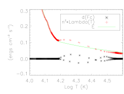
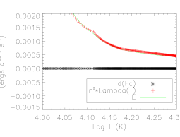
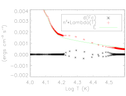
Figure 4: Top panel, left: temperature (solid line) and pressure (dashed line) as a function of the curvilinear coordinate along the field lines, $s$. Right: divergence of the conductive flux (asterisks), radiative losses (crosses) and heating rate, $E$ (solid line), as a function of the temperature, for loop 13. Middle and bottom panels: as in the top panels for loop 16 and 22, respectively.

Table 2: As in Tab. 1 for intermediate-temperature loops ($\gamma=1$).

Loop	$E_{\mathrm{h}}$	$T_{\mathrm{max}}$	$P$	$L/2$	$h$
	$10^{-4}$ ergs cm-3 s-1	MK	dyne cm-2	Mm	Mm
Loopi: 17
	0.2	0.242	0.008	7	1.12
25	5	0.206	0.008	8.9	3.14
26	10	0.431	0.036	9.2	3.44

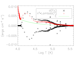
Figure 5: Top panel, left: temperature (solid line) and pressure (dashed line) as a function of the curvilinear coordinate along the field lines, $s$. Right: divergence of the conductive flux (asterisks), radiative losses (crosses) and heating rate, $E$ (solid line), as a function of the temperature, for loop 26.

Using the same radiative loss function and $\gamma=1$, we also obtained quasi-static intermediate-temperature loops ($0.1<T<0.5\times 10^{5}$ MK), listed in Table 2. These loops are obtained by starting the simulations from the quasi-static cool loop 17 of Table 1 in Paper I. For loop 26, we show in Fig. 5 the behavior of the temperature and the pressure as a function of $s$ (left) and of the terms of the energy equation as a function of the temperature (right). The divergence of the conductive flux, comparable to the radiative losses, contributes to dissipate the heating in excess.

3.3 Relations between loop parameters and scaling laws

In Fig. 6 we show the relations between the thermodynamic parameters ($P$, $T_{\mathrm{max}}$ and $L/2$) and $E_{\mathrm{h}}$ for the loops in Table 1 (loops 1–3 are represented by triangles, loops 4–15 by crosses, loops 16–18 by asterisks, and loops 19–24 by diamonds) and Table 2 (represented by squares). The solid lines in the lower panels of Fig. 6 represent the “static” scaling laws for coronal loops described by Rosner et al. (1978, hereafter RTV) for different values of $L/2$. The pressure of all cool loops with $T<0.1$ MK is proportional to $E_{\mathrm{h}}$ and it is dependent on their length and maximum temperature. In the simulations, indeed, we increase $E_{\mathrm{h}}$ in order to have higher temperature loops, obtaining also higher pressure and longer loops. There is, however, a maximum limit of $E_{\mathrm{h}}$ (different for each initial condition-loop) at which, even increasing its value, the loops continue increasing their pressure but not their maximum temperature (see bottom-left panel of Fig. 6).

Intermediate-temperature loops obey the RTV scaling law for coronal loops for temperature and pressure (see bottom-left panel of Fig. 6) as the intermediate-temperature loops we found in Paper I. Observed intermediate-temperature loops do not obey the coronal scaling laws (Brown 1996), but as we already discussed in Paper I, the static model used by Rosner et al. (1978) to derive the relationships between coronal temperature, pressure, length and heating in coronal loops does not seem to accurately predict the physical conditions of these loops. We obtained intermediate-temperature loops with pressures that are 1–2 orders of magnitudes lower than measured in observed loops with the same temperatures (Brown 1996). Loops 25–26 have the right pressures to fall on the scaling laws lines.

Figure 6: Behavior of the physical parameters for loops 1–3 (triangles), 4–15 (crosses), 16–18 (asterisks), and 19-24 (diamonds) of Table 1, and loops 25–26 (squares) of Table 2. The solid lines represent the RTV scaling laws for coronal loops for different values of L/2.

3.4 Calculated DEMs for cool and intermediate-temperature loops

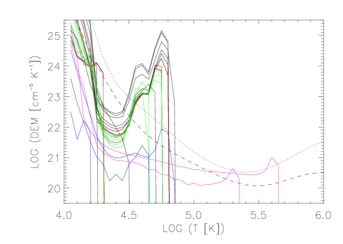
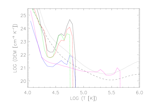
Figure 7: Top: Calculated DEMs for the quasi-static cool loops 1–3 (solid blue lines), 4–15 (black), 16–18 (red), 19–24 (green) of Table 1, and the intermediate-temperature loops 25–26 (magenta) of Table 2, compared to the DEMs of the quiet Sun (dashed) and active region (dotted) from the “CHIANTI” atomic data base (Dere et al. 2009). Bottom: total DEMs for each group of loops shown in the top panel.

Figure 8: Total DEM resulting from the combination of the DEMs of the loops 1–24 and 25–26 (solid line), compared to the DEMs of the quiet Sun (dashed) and active region (dotted) from the “CHIANTI” atomic data base (Landi et al. 2013).

The theoretical DEMs for a single or isolated loop were computed for the quasi-static loops we found according to Spadaro et al. (2003), with a temperature bin of 0.05 dex on a $\log T$ scale along the loop:

$$DEM=n^{2}\frac{ds}{dT}.$$ (15)

This simplified approach permits to study the overall properties of the DEM of this class of loops without the need for taking into account details such as the shape of the loop, the geometry of the observations, the loop cross-section, etc.

The upper panel of Fig. 7 shows the calculated DEMs versus temperature of the quasi-static cool loops 1–3 (solid blue lines), 4–15 (black), 16–18 (red), 19–24 (green) of Table 1, and the quasi-static intermediate-temperature loops 25–26 (magenta) of Table 2. In this figure and in the next ones, we plot, for comparison, the observed DEMs of the quiet Sun and active region (dashed and dotted lines, respectively), derived using the Vernazza & Reeves (1978) average quiet Sun and active region intensities, and produced as part of the “CHIANTI” atomic data base collaboration (Landi et al. 2013). In the lower panel of Fig. 7 we plot the total theoretical DEMs for each group of loops obtained starting from a different initial loop-condition (distinguished by the different colors). Assuming that the loops are equiprobable (uniformly distributed in $\log T$) and with the same cross-section, we divided the temperature range into bins of amplitude $0.2$ dex on a $\log T$ scale, and considered for each bin a representative loop, i.e. a loop whose maximum temperature belongs to that bin (our loops are almost isothermal). The total DEMs are obtained by summing the DEMs of these representative loops. When more loops have their maximum temperature falling in the same bin, we averaged their DEMs.

Using $\Lambda_{\mathrm{kp}}$ (and $\gamma=1$), we obtain cool loops with maximum temperatures covering the temperature range up to the position of its peak ($\log T\sim 4.8$ K) except for the interval $4.3\lesssim\log T\lesssim 4.5$. Adding the DEMs of the intermediate-temperature loops 25–26, the resulting DEM (black solid line in Fig. 8) follows the shape of the observed ones, except for the interval $4.6\lesssim\log T\lesssim 4.8$, where we have an excess of emission due to the high density of the loops with maximum temperature falling in that interval. Only Loop 2 and 3, with maximum temperature belonging to this interval, have a pressure such that their DEMs would resemble the observed one, but the solar total pressures at these temperatures and heights, according to the model of Avrett & Loeser (2008) are estimated around 0.1 dyne cm^-2 that is much higher than the pressures of loops 2 and 3 and closer to that of all other loops of Table 1. Moreover, the presence of the Ly-$\alpha$ peak at log$T\sim 4.2$ K and, in particular, the negative slope of the radiative loss function (as explained in Sec. 2.2), produces a relative minimum in all DEMs, which remains in the total DEM (lower panel of Fig. 7, blue, black, green or red lines). There are, however, in the literature, derived quiet Sun DEMs (Macpherson & Jordan 1999) that exhibit a minimum around log$T\sim 4.2$ K.

There is a minimum in the total DEM also around log$T=4.9$ K that is caused by the lack of cool loops with that maximum temperature. This minimum almost corresponds to the maximum of the function $\Lambda_{\mathrm{kp}}$ or better to the point where its slope starts to change and we have $a<1$. So, the lack of cool loops with maximum temperature around $\log T=4.9$ K it is not caused by an incomplete exploration of the parameter space but by the negative slope of $\Lambda_{\mathrm{kp}}$ that prevents their formation. However, the shape of the averaged DEM of the loops 25–26, with a flat minimum and a tail extended towards low temperatures, helps filling this gap, improving the agreement with the observed DEM. Since we considered a filling factor of $100\%$ the total DEM has its highest value. With a lower filling factor the height of the DEM would be lower.

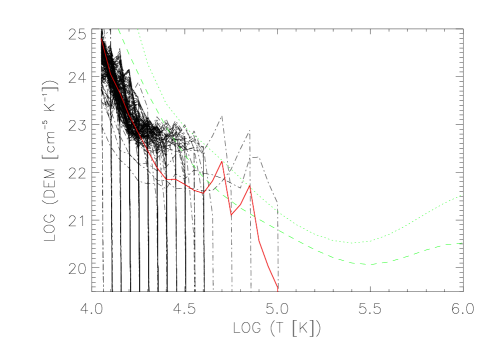
Figure 9: Calculated DEM of Loop0 over the first 42 min of the simulation (red line). It is obtained by averaging the DEM of each loop obtained at each time step of the simulation (black dash-dotted lines). It is compared to the DEMs of the quiet Sun (green dashed line) and active region (green dotted line) from the “CHIANTI” atomic data base (Landi et al. 2013).

We calculate also the emission due to Loop0, obtained in Sect. 3.1 by performing a simulation using constant heating rate per unit volume ($\gamma=0$) and starting from a quasi-static cool loop of maximum temperature $T_{\mathrm{max}}\sim 1.2\times 10^{4}$ K. The loop becomes a quasi-static “coronal” loop, after $\sim 2.5$ h from the beginning of the simulation, reaching a top temperature of $\sim 8.5\times 10^{5}$ K. The evolution of Loop0’s mean temperature, density and pressure is shown in Fig. 3.

The discussion that follows is based on considering each recordered step of the simulation as a single dynamic loops at a particular instant of its evolution (for example, cooling down or heating up depending if we keep the heating on or we shut it down). We show in Fig. 9, indeed, the DEM of each loop obtained at each time step of the simulation (black dot-dashed lines) during the first 42 min in which Loop0 evolves keeping its temperature lower than $10^{5}$ K. The red line is the total DEM obtained by combining all the loops as already explained. Another possible way to calculate the total DEM is described in Susino et al. (2010). They simulated the DEM of a multi-stranded loop by averaging instantaneous DEMs calculated at n different times, randomly selected throughout the simulation. This approach is based on the assumption that the states of the model at n randomly selected times can be used to describe the behaviour of n independent strands observed at the same time. In this analysis, we do not want to concentrate on how the loops are obtained but we only want to show how the emission measure produced by this particular distribution of loops looks like. The total DEM resembles quite well the observed one and we do not have any of the problems observed with the total DEM obtained from static loops. We are able to obtain also loops with maximum temperature prohibitive for the quasi-static loops ($\log T\sim 4.2$ and $\sim 4.9$ K).

Obviously, the resulting DEM depends on the assumption we are making, in particular on the number of the loops that fall in a certain temperature interval and/or the filling factor and, obviously, it depends on the distribution of the loops, and, ultimately, on the distribution of the heating rates (Antiochos & Noci 1986).

3.5 Non-equilibrium phase of Loop0

We have furthermore examined the behaviour of the vertical component of velocites in Loop0. At each time step of the simulation we computed the mean value weighted by the DEM (e.g.: Spadaro et al. 2003) of the vertical component of velocities in temperature bins of 0.20 dex in $\log T$, considering separately the two halves of the loop. The temperature bins chosen are centered at $\log T=4.1$, $4.3$, $4.5$, $4.7$, and $4.9$. The last two bins are populated only towards the end of the transient phase. We found that in the transient phase we are considering, the vertical velocities are of the same magnitude and sign at both footpoints.

During the transient phase, the mean vertical component of velocities averaged on the whole loop for the different temperature bins appear in a few bursts lasting 1-4 minutes and reaching values of the order of 5-10 km/s or more in absolute value. After the first 10-15 minutes of the simulation,the velocities in these bursts are sistematically negative, adopting a sign convention which corresponds to negative Doppler shifts (redshifts). Considering the episodic character of these Doppler shifts, the average values in each temperature bin over the 42 minutes interval correspond to redshifts of the order of -1 km/s or less. These redshifts, however, are limited to the range of temperatures covered by the transient phase (see Fig. 9). At later times, as the loop reaches near coronal temperatures, the vertical velocities start to oscillate between blue- and red-shifts, with decreasing amplitudes until a quasi-static situation is attained. Peter & Judge (1999) report observed values of about -5 km/s in the range $\log T=4.5-5$, with one exception of nearly zero wavelength shift. These redshifts are higher than our average redshifts, even though it should be noted that there are only a few measurements in the temperature range best covered by the transient phase of the simulations ($\log T<4.6$). Their Table 3 lists only three lines nominally forming at or below $\log T=4.7$, i.e. He i 584 Å, C ii 1036 Å and C ii 1037 Å. It is however encouraging that our results for transient phase of Loop0 show a predominance of redshifts, although this result should be confirmed and extended with simulations spanning a variety of loop parameters.

4 Conclusions

We have studied the conditions of existence and stability of cool loops with $T\lesssim 0.1$ MK through hydrodynamic simulations, introducing an optically thick radiative loss function. We analyzed two different cases: constant heating rate either per volume or per particle. We found that it is possible to obtain quasi-static (velocities lower than $1$ km/s) cool loops, as predicted by Antiochos & Noci (1986), only by using a constant heating rate per particle, unlike the previous work in which we used different radiative loss functions, with a less pronounced Ly-$\alpha$ peak.

We also obtained quasi-static loops with maximum temperature in the range $1-5\times 10^{5}$ K, using the same optically thick radiative loss function. These loops are smaller with respect to coronal loops but have different characteristics compared to the static cool loops proposed by Antiochos & Noci (1986) and others. They obey the scaling laws for coronal loops contrary to results of previous works based on the observational data (e.g., Brown 1996). The loops obtained have indeed low pressures that make their parameters obey the RTV scaling laws, but these pressures are 1–2 orders of magnitudes lower than those estimated from observations (Brown 1996).

We examined and discussed the quasi-static solutions we found and analyzed the contributions of the cool and intermediate-temperature loops to the TR DEM, finding that a combination of these loops (assuming that they were uniformly distributed), precisely because of their computed pressures, can give a DEM with a shape not too far from the observed one for $\log T<4.3$ and $\log T>5.0$. However there is a pronounced excess emission due to the high density of the cool loops between $4.6\lesssim\log T_{\mathrm{max}}\lesssim 4.8$ and a deficit around $\log T\sim 4.4$ (see Sec. 2.2).

In this work we also showed a dynamic loop (Loop0), obtained by performing a simulation using constant heating rate per unit volume and starting from a quasi-static cool loop of maximum temperature $T_{\mathrm{max}}\sim 1.2\times 10^{4}$ K. The loop becomes a quasi-static “coronal” loop, after $\sim 2.5$ h from the beginning of the simulation, reaching a top temperature of $\sim 8.5\times 10^{5}$ K. While the final state does not reproduce the observed DEM for temperatures lower than $10^{5}$ K, the average DEM of Loop0, interpreted as a combination of a set of evolving dynamic loops, reproduces quite well the observed DEM. The whole simulation that we called “Loop0” can also be considered as the evolution of a single loop emerging from lower atmospheric layers to the corona. The dimensions of this emerging loop, its initial and final temperatures, and the time-scale of the event are comparable to the observations and simulations of an emerging magnetic loops from photosphere to low corona as the one described in the work of Guglielmino et al. (2010).

In principle, cool and intermediate-temperature loops could be observed with current telescopes, but in order to resolve them in all their temperature extension, we would need multi-temperature observations, i.e. different UV lines formed at temperatures between $0.01-1$ MK with resolution of at least 1”. Highly dynamical cool, low-lying loops have recently been reported by Hansteen et al. (2014) using observations obtained with the IRIS spacecraft (De Pontieu et al. 2014). That kind of loops are usually observed as time-dependent, short-lived “segments”, not as complete loops. This could depend on the fact that those loops extend over a range of temperatures not enterely covered by the IRIS spectral lines. Such observations suggest that the class of loops reported by Hansteen et al. (2014) is related to short-lived, episodic heating; “temporary” loops would therefore be created and then rapidly collapse. Hansteen et al. also stress that these are high-density structures and postulate that these loops follow near-horizontal magnetic field (hence: they are low-lying).

Based on the work of Antiochos & Noci (1986) and Paper I, we expect cool loops to be low-lying even though we focuse our attention on steady-state heating. In this work, we confirm that the existence, stability and properties of cool loops strongly depend on the details of the radiative loss function. We also find that considering a more realistic function, the derived DEMs depart from the observations (see Fig. 7). On the other hand, transient loops, like Loop0, display characteristics which are appealingly closer to observations. Note that this class of transient loops does not necessarily imply impulsive heating. The similarity between the DEM of the transient phase of Loop0 and the observed one, together with the new observations of dynamic small scale structures on the Sun, suggest us to focus our attention to simulate dynamic cool loops. This conclusion is reinforced by noting that this dynamical loop is characterized in its non-equilibrium phase by the predominance of redshifts at its footpoints appearing in bursts of the order of -5 – -10 km/s and in average of the order of -1 km/s or less over the 42 minutes of the transient. Redshifts of this magnitude could be marginally consistent with existing spectroscopic observations of redshifts in the transition region in the relative low temperature range best covered by the transient phase of the simulation ($\log T<4.6$). The episodic nature of these red-shifts could be investigated by IRIS time-resolved spectroscopic observations. We also plan to further investigate this intriguing result with more simulations spanning a wider range of loop parameters.

In this perspective, an important point to consider is the effects of partial ionization of hydrogen on the hydrodynamics of the loop plasma. The equations for mass, momentum and energy conservation adopted in our work are for a fully ionized hydrogen plasma. This assumption is well verified in our cool loops, which are characterized by plasma pressures in the range $10^{-2}-10^{-1}$ dyne cm^-2, according to the calculations reported in Table 3 of Kuin & Poland (1991). Only in three cases the pressure in the loop is above $10^{-1}$ dyne cm^-2, resulting in a significant fraction of neutral hydrogen just below 2$\times 10^{4}$ K (see Kuin & Poland 1991). Note that the fraction increases and becomes important even at higher temperatures as the pressure becomes higher. Since Hansteen et al. (2014) stress that the episodically heated loop they observe are high-density structures, the simulation of dynamic cool loops should take into account the fraction of neutral hydrogen in the hydrodynamic equations.