Hybrid 3D Localization for Visible Light Communication Systems

Abstract

In this study, we investigate hybrid utilization of angle-of-arrival (AOA) and received signal strength (RSS) information in visible light communication (VLC) systems for 3D localization. We show that AOA-based localization method allows the receiver to locate itself via a least squares estimator by exploiting the directionality of light-emitting diodes (LEDs). We then prove that when the RSS information is taken into account, the positioning accuracy of AOA-based localization can be improved further using a weighted least squares solution. On the other hand, when the radiation patterns of LEDs are explicitly considered in the estimation, RSS-based localization yields highly accurate results. In order to deal with the system of non-linear equations for RSS-based localization, we develop an analytical learning rule based on the Newton-Raphson method. The non-convex structure is addressed by initializing the learning rule based on 1) location estimates, and 2) a newly developed method, which we refer as random report and cluster algorithm. As a benchmark, we also derive analytical expression of the Cramér-Rao lower bound (CRLB) for RSS-based localization, which captures any deployment scenario positioning in 3D geometry. Finally, we demonstrate the effectiveness of the proposed solutions for a wide range of LED characteristics and orientations through extensive computer simulations.

I Introduction

The reliable positioning in the environments where the Global Positioning System (GPS) signals cannot easily penetrate has become a growing research area due to its numerous applications [1]. Among many other technologies, radio frequency identification (RFID)[2, 3, 4], ultra wideband (UWB) positioning [5], cellular or wireless local area network (WLAN) based positioning [6, 7], and fingerprint based localization techniques [8] are the most prominent ones for GPS-free localization. Beside those technologies, visible light communication (VLC) [9, 10, 11], which has been recently emerging as a promising technology to provide high data rates for short range communications, can also deliver high accuracy for 3D localization [12, 13].

VLC systems have numerous advantages in comparison to other legacy systems. First, the performance of VLC systems is not affected by the radio frequency (RF) interference. Moreover, multipath fading can be averaged out as the area of photodetectors are very large compared to wavelength of the visible light [14]. Second, light emitting diodes offer narrow beamwidth, which enables more accurate angle of arrival information at the receiver side [15, 16]. Third, VLC systems can be utilized in scenarios where RF radiation is potentially hazardous or even forbidden such as planes or hospitals. Lastly, VLC systems maintain maintains high data rate communications while simultaneously providing illumination.

Due to its aforementioned advantages, employing VLC systems for the localization is recently getting significant attention in the literature. In particular, two approaches have become prominent for VLC-based localization: angle of arrival (AOA) based methods [16, 15] and received signal strength (RSS) based methods [17, 18]. While AOA-based approach takes the direction information of LED transmitters, RSS-based localization considers the captured power from LED transmitters. For example, in [15], AOA-based localization is investigated for indoor scenarios and a connectivity-based solution is proposed under 2D settings. The proposed solution exploits the narrow field of view (FOV)s of LEDs and relies on that fact that the receiver is likely to be located at the intersection of the directions of the connected LEDs transmitters. Yet, the proposed method is valid only under 2D settings where two straight lines always intersect between each other unless they are not parallel to each other. In [16], AOA information of LED transmitters are exploited in an ad-hoc networking environment. By starting from a limited number GPS-enabled devices, each node discovers its own location and broadcasts this information in order to help the other nodes to find their own locations. In [17], an RSS-based indoor positioning algorithm based on preinstalled LED transmitters is proposed to estimate receiver locations by analytically solving the equations that characterize the Lambertian pattern [19]. However, the analytical derivations are not generic, and cover only a limited number of scenarios, where the directionality of the LEDs (i.e., their modes) and the receiver’s direction are fixed to some predetermined values. In [18], Cramér-Rao lower bound (CRLB) for RSS-based localization is derived for a specific scenario of LED transmitters and receiver positions, where the authors emphasize the complexity of obtaining the CRLB in a 3D geometry.

In this study, we evaluate AOA-based and RSS-based localization methods by using multi-element visible light access points which consist of several LED transmitters [10, 20, 21]. The main contributions of this paper are as follows:

• Hybrid Localization: We develop hybrid localization methods that utilize both AOA and RSS information in the estimation process to improve the positioning accuracy in VLC systems. For AOA-based localization, we show that the VLC receiver can estimate its own location via a least squares (LS) estimator and the positioning accuracy can be improved further by incorporating with the RSS information. In addition, we demonstrate that the outcome of AOA-based location estimation can effectively be useful to deal with the non-convex objective function in RSS-based localization.

• Theoretical Framework: We introduce a comprehensive theoretical framework that allows us to investigate the various hybrid localization methods for VLC and the impact of the orientations of LED transmitters and the physical characteristics of LEDs on the estimator performance. As opposed to earlier work in the literature, the proposed methods and theoretical investigations are generic, and applicable to any 3D topology. Based on the introduced framework, we discuss the optimal LED weighting problem for AOA-based localization and the non-convex objective function for RSS-based localization. As a benchmark, we derive the analytical expression of CRLB for RSS-based localization, which generalizes the derivations provided in [18]. By using the derived CRLB, we demonstrate the trade-offs between light distribution and localization accuracy distribution and discuss the impact of LED characteristics, such as directivity, density, and orientation, on the maximum achievable positioning accuracy.

• Learning Algorithms: We introduce two algorithms, i.e., analytical learning algorithm based on Newton-Raphson method and random report and cluster (RRC) algorithm, to combat with the system of non-linear equations and the non-convex structure of the objective function for RSS-based localization, respectively. In order to increase the likelihood that the Newton-Raphson method converges to the global optimum, we employ RRC algorithm and show its effectiveness numerically.

The rest of the paper is organized as follows. The system model which captures any VAP deployment scenario in 3D geometry is provided in Section II. AOA-based localization and hybrid utilization of AOA and RSS information for VLC systems are discussed in Section III. Subsequently, RSS-based localization is investigated in Section IV. Theoretical expression of CRLB for RSS-based localization, the analytical learning rule, and the RRC algorithm are provided in this section. The numerical results evaluating the performance of the proposed methods for different configuration of VAPs are given in Section V. Finally, some concluding remarks are indicated in Section VI.

Notations: ${\rm\bf I}_{K}$ is the $K\times K$ identity matrix. The transpose operation is denoted by $(\cdot)^{\rm T}$. The Moore-Penrose pseudoinverse operation is denoted by $(\cdot)^{\rm\dagger}$. The operation of $\lVert{\cdot}\rVert_{2}$ is the 2-norm of its argument. The vectorization and the expectation operators are denoted by ${\rm vec}\left(\cdot\right)$ and $\mathbb{E}\left[{\cdot}\right]$, respectively. The kernel of a matrix is represented by $\ker\left(\cdot\right)$. The field of real numbers is shown as $\mathbb{R}$. $\mathcal{N}\left(0,{\rm\bf C}\right)$ is the Gaussian distribution with zero mean and covariance matrix of ${\rm\bf C}$.

II System Model

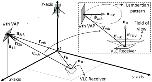
Figure 1: System model with multiple VAPs and a single VLC receiver.

We consider $K$ VAPs communicating with a VLC receiver as illustrated in Figure 1. Without loss of generality, the location of the receiver and its orientation are denoted by ${\rm\bf r}_{\rm R}=[x,y,z]^{\rm T}\in\mathbb{R}^{3\times 1}$ and ${\rm\bf n}_{\rm R}=[{n}_{{\rm R}}^{(x)},{n}_{{\rm R}}^{(y)},{n}_{{\rm R}}^{(z)}]^{\rm T}\in\mathbb{R}^{3\times 1}$ in Cartesian coordinate system, respectively. We consider multi-element VAPs which consist of $M$ LED transmitters. The location of $m$th LED transmitter of $k$th VAP and its orientation are denoted by ${\rm\bf r}_{mk}=[x_{mk},y_{mk},z_{mk}]^{\rm T}\in\mathbb{R}^{3\times 1}$ and ${\rm\bf n}_{mk}=[{n}_{{mk}}^{(x)},{n}_{{mk}}^{(y)},{n}_{{mk}}^{(z)}]^{\rm T}\in\mathbb{R}^{3\times 1}$, respectively. By assuming transmit power of $1$ W for each LED transmitter, the signal power of the $m$th LED of $k$th VAP at the receiver is given by [19]

$${P_{mk}}=\frac{n+1}{2\pi} \cos^{n}(\phi_{mk})\cos(\theta_{mk})\frac{A_{\rm R}}{R_{mk}^{2}}$$

$$~{}~{}~{}~{}~{}~{}~{}~{}~{}~{}~{}~{}~{}~{}~{}~{}\times{\Pi}\left(\frac{\theta_{mk}}{\theta_{\rm FOV}}\right){\Pi}\left(\frac{\phi_{mk}}{\pi/2}\right)~{},$$ (1)

where $\phi_{mk}$ is the angle between the LED transmitter orientation vector and the incidence vector, $\theta_{mk}$ is the angle between receiver orientation vector and the incidence vector, $R_{mk}$ is the distance between the LED transmitter and the receiver, $A_{\rm R}$ is the area of photo detector (PD) in ${\rm m}^{2}$, $\theta_{\rm FOV}$ is the FOV of PD, $n$ is the mode number which specificities the directionality of LED, and ${\Pi}\left(\cdot\right)$ is the rectangle function defined as

$${\Pi}\left(x\right)\triangleq\begin{cases}1&\mbox{for }|x|\leq 1\\ 0&\mbox{for }|x|>1\end{cases}~{}.$$ (2)

While ${\Pi}\left({\theta_{mk}}/{\theta_{\rm FOV}}\right)$ in (1) implies that a VLC receiver can detect the light only when $\theta_{mk}$ is less than $\theta_{\rm FOV}$, ${\Pi}\left({\phi_{mk}}/{(\pi/2)}\right)$ ensures that the location of VLC receiver is in the FOV of LED transmitter. Let ${\rm\bf v}_{mk}={\rm\bf r}_{\rm R}-{\rm\bf r}_{mk}=[{a}_{mk},{b}_{mk},{c}_{mk}]^{\rm T}\in\mathbb{R}^{3\times 1}$ be the incidence vector between the receiver and the $m$th LED transmitter of $k$th VAP. Then, the parameters of (1) can be expressed as

$$R_{mk}=\lVert{{\rm\bf v}_{mk}}\rVert_{2}~{},$$ (3)

$$\cos(\phi_{mk})=\frac{{\rm\bf n}_{mk}^{\rm T}({\rm\bf r}_{\rm R}-{\rm\bf r}_{mk})}{R_{mk}}=\frac{{\rm\bf v}_{mk}^{\rm T}{\rm\bf n}_{mk}}{\lVert{{\rm\bf v}_{mk}}\rVert_{2}}~{},$$ (4)

and

$$\cos(\theta_{mk})=\frac{{\rm\bf n}_{\rm R}^{\rm T}({\rm\bf r}_{mk}-{\rm\bf r}_{\rm R})}{R_{mk}}=-\frac{{\rm\bf v}_{mk}^{\rm T}{\rm\bf n}_{\rm R}}{\lVert{{\rm\bf v}_{mk}}\rVert_{2}}~{}.$$ (5)

Therefore (1) can be rewritten as

$${P_{mk}}=-\frac{(n+1)A_{\rm R}}{2\pi}{\Pi}\left(\frac{\theta_{mk}}{\theta_{\rm FOV}}\right){\Pi}\left(\frac{\phi_{mk}}{\pi/2}\right)\times f\left({\rm\bf v}_{mk}\right)~{},$$ (6)

where

$$f\left({\rm\bf v}_{mk}\right)= \frac{({\rm\bf v}_{mk}^{\rm T}{\rm\bf n}_{mk})^{n}{\rm\bf v}_{mk}^{\rm T}{\rm\bf n}_{\rm R}}{\lVert{{\rm\bf v}_{mk}}\rVert_{2}^{n+3}}$$

$$= ({a}_{mk}{n}_{{mk}}^{(x)}+{b}_{mk}{n}_{{mk}}^{(y)}+{c}_{mk}{n}_{{mk}}^{(z)})^{n}$$

$$~{}~{}~{}~{}~{}~{}~{}~{}~{}\times\frac{({a}_{mk}{n}_{{\rm R}}^{(x)}+{b}_{mk}{n}_{{\rm R}}^{(y)}+{c}_{mk}{n}_{{\rm R}}^{(z)})}{({a}_{mk}^{2}+{b}_{mk}^{2}+{c}_{mk}^{2})^{\frac{n+3}{2}}}~{}.$$ (7)

It is worth noting that (6) includes only the line-of-sight (LOS) component, i.e., first order Lambertian pattern, since the LOS component of signal is dominant compared to other multipath components for VLC systems [19, 17]. Hence, we discuss the theoretical analyses given in the following sections based on LOS component. In this study, we assume that all LEDs in VAPs are identical. In addition to that, the locations of the transmitters and directions of each LED are assumed to be known at the receiver, which can be shared through periodic broadcast messages. The unique identity of each LED transmitter and its corresponding VAP are assumed to be decodable at the receiver, which can be achieved by assigning different codes/headers from each LED transmitter. Accordingly, it is assumed that the receiver is able to measure the RSS associated with each LED transmitter.

III AOA-Based Localization

In AOA-based localization, a VLC receiver selects one of the LED transmitters for each VAP based on the RSS information and locates itself by exploiting the orientations of LED transmitters. Geometrically, AOA-based localization relies on finding a point in 3D space such that it minimizes the sum of distances (or squared distances) between this point and all the other lines extended from the directions of LED transmitters selected by the receiver [16, 15]. This approach can allow the receiver to locate itself with only two anchor nodes when the receiver is close to the intersection of the corresponding LED directions.

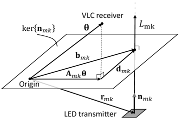
Figure 2: The distance between VLC receiver’s location and the line extended by the direction of an LED transmitter.

In order to analyze the AOA-based localization, let $L_{mk}$ be the line associated with the $m$th LED transmitter of $k$th VAP as illustrated in Figure 2, where its origin and direction are captured by the vectors ${\rm\bf r}_{mk}$ and ${\rm\bf n}_{mk}$, respectively. In addition, let ${\rm\bf A}_{mk}\in\mathbb{R}^{3\times 3}$ be the projection matrix which projects every vector ${\rm\bf x}\in\mathbb{R}^{3\times 1}$ onto the null space of ${\rm\bf n}_{mk}$, i.e., $\ker\left({\rm\bf n}_{mk}\right)$, which can be calculated by ${\rm\bf A}_{mk}={\rm\bf I}_{3}-{\rm\bf n}_{mk}{\rm\bf n}_{mk}^{\rm T}$. Hence, any vector in the column space of ${\rm\bf A}_{mk}$ is orthogonal to the direction of $L_{mk}$. In particular, the projection of any point on $L_{mk}$ yields the same point, i.e., the intersection between $L_{mk}$ and the subspace spanned by the columns of ${\rm\bf A}_{mk}$. The intersection point ${\rm\bf b}_{mk}$ can be simply calculated as ${\rm\bf A}_{mk}{\rm\bf r}_{mk}$ since ${\rm\bf r}_{mk}$ is a point on $L_{mk}$. Hence, the distance vector between an arbitrary point ${\bm{\uptheta}}\in\mathbb{R}^{3\times 1}$ and $L_{mk}$ is given by ${\rm\bf d}_{mk}={\rm\bf b}_{mk}-{\rm\bf A}_{mk}{\bm{\uptheta}}$, which yields

$${\rm\bf b}_{mk}={\rm\bf A}_{mk}{\bm{\uptheta}}+{\rm\bf d}_{mk}~{}.$$ (8)

By stacking the set of equations related to LED transmitters, we obtain

$${\rm\bf b}={\rm\bf A}{\bm{\uptheta}}+{\rm\bf d}~{},$$ (9)

where

$${\rm\bf b}=\begin{bmatrix}{\rm\bf b}_{{s_{1}}1}\\ \vdots\\ {\rm\bf b}_{{s_{k}}k}\\ \vdots\\ {\rm\bf b}_{{s_{K}}K}\\ \end{bmatrix},~{}{\rm\bf A}=\begin{bmatrix}{\rm\bf A}_{{s_{1}}1}\\ \vdots\\ {\rm\bf A}_{{s_{k}}k}\\ \vdots\\ {\rm\bf A}_{{s_{K}}K}\\ \end{bmatrix},~{}{\rm\bf d}=\begin{bmatrix}{\rm\bf d}_{{s_{1}}1}\\ \vdots\\ {\rm\bf d}_{{s_{k}}k}\\ \vdots\\ {\rm\bf d}_{{s_{K}}K}\\ \end{bmatrix}~{},$$ (10)

and $s_{k}$ is the index of selected LED transmitter of $k$th VAP. Therefore the objective function which minimizes the sum of squared error is solved via an LS estimator given by

$$\tilde{{\rm\bf r}}_{\rm R} ={{\rm\bf A}^{\rm\dagger}}{\rm\bf b}~{}.$$ (11)

III-A Weighting LED Transmitters

Treating the AOA information obtained from each of the LED transmitters identically, as in (11), may cause significant positioning error since the distance between exact position of the receiver and the line extended by the direction of LED transmitter may be large in some cases. In other words, less reliable AOA information may bias the location estimation and degrade localization accuracy. In order to address this issue, we consider an objective function which minimizes the weighted sum of squared distance as

$$\tilde{{\rm\bf r}}_{\rm R} =\arg\min_{{\bm{\uptheta}}}\sum_{\begin{subarray}{c}k=1\\ m=s_{k}\end{subarray}}^{K}\beta_{mk}\lVert{{\rm\bf d}_{mk}}\rVert_{2}^{2}$$

$$=\arg\min_{{\bm{\uptheta}}}\sum_{\begin{subarray}{c}k=1\\ m=s_{k}\end{subarray}}^{K}\beta_{mk}\lVert{{\rm\bf A}_{mk}{\bm{\uptheta}}-{\rm\bf b}_{mk}}\rVert_{2}^{2}~{},$$ (12)

where $\beta_{mk}$ is the weighing factor for the distance between ${\bm{\uptheta}}$ and $L_{mk}$. The purpose of weighing factors is to take the variability of ${\rm\bf d}_{mk}$ into account in the optimization. Under the assumptions of $\mathbb{E}\left[{{\rm\bf d}_{mk}}\right]=0$ and $\mathbb{E}\left[{{{\rm\bf d}_{nl}^{\rm T}}{{\rm\bf d}_{mk}}}\right]=0$, according to Gauss-Markov theorem [22], the optimal weighting factors that yield minimum variance estimator for (12) is obtained as

$$\beta_{mk}=c_{0}\times\frac{1}{\mathbb{E}\left[{\lVert{{\rm\bf d}_{mk}}\rVert^{2}}\right]}~{}.$$ (13)

where $c_{0}$ is an arbitrary positive real number. In order to calculate (13), the statistical characteristics of ${{\rm\bf d}_{mk}}$ should be known a priori. To this end, we exploit RSS information associated with LED transmitters in this study.

Without loss of generality, consider an LED transmitter located at the origin and its orientation is set to ${\rm\bf n}_{0}=[0,0,1]^{\rm T}$. Assuming that the LED transmitter and the VLC receiver face each other, i.e., ${\rm\bf n}_{\rm R}=-{\rm\bf n}_{0}$, $\theta_{\rm FOV}=\pi/2$, and ${\phi_{mk}}\leq{\pi/2}$, we rewrite (6) as

$${P_{0}}=\frac{(n+1)A_{\rm R}}{2\pi}\frac{z^{n+1}}{(x^{2}+y^{2}+z^{2})^{\frac{n+3}{2}}}~{}.$$ (14)

We then obtain the identity which characterizes the distance between the LED direction and VLC receiver’s location as

$$\lVert{{\rm\bf d}_{0}}\rVert_{2}^{2}=C^{{{\frac{2}{n+3}}}}z^{\frac{2n+2}{n+3}}-{z^{2}}~{},$$ (15)

where $\lVert{{\rm\bf d}_{0}}\rVert_{2}^{2}=x^{2}+y^{2}$ and $C\triangleq\frac{(n+1)A_{\rm R}z}{2\pi{P_{0}}}$. It is worth noting that (15) also identifies the locations where VLC receiver could observe the same RSS and forms an RSS contour. For example, when ${P_{0}}$ is fixed to $0.1$ mW and $A_{\rm R}=1$ cm², the potential locations of a VLC receiver are shown in Figure 3 for a given LED mode. Under the assumption that the receiver is equally likely to be on the locations that satisfy (15), one should obtain $\mathbb{E}\left[{\lVert{{\rm\bf d}_{0}}\rVert_{2}^{2}}\right]$ in order to find optimal weights given in (13). However, the calculation of $\mathbb{E}\left[{\lVert{{\rm\bf d}_{0}}\rVert_{2}^{2}}\right]$ is not trivial due to nonlinear characteristics of (15). On the other hand, considering the narrow beamwidth of the LED with high modes, RSS contours are spread around on $z$-axis as shown in Figure 3. Therefore, it becomes more likely that the VLC receiver location far away from the LED direction. Hence, in this study, we approximate the exact distribution of $\lVert{{\rm\bf d}_{0}}\rVert_{2}$ with a uniform probability density function (PDF) given by

$$p\left(\lVert{{\rm\bf d}_{0}}\rVert_{2}\right)=\begin{cases}\frac{1}{2\pi d_{\rm max}},&\lVert{{\rm\bf d}_{0}}\rVert_{2}=d_{\rm max}\\ 0,&{\rm otherwise}\\ \end{cases}$$ (16)

where

$$d_{\rm max}=\max\left({\lVert{{\rm\bf d}_{0}}\rVert_{2}}\right)=\sqrt{B^{-\frac{n+1}{2}}C-B^{-\frac{n+3}{2}}C}$$ (17)

and $B\triangleq(2n+6)/(2n+2)$. Therefore the variance of $\lVert{{\rm\bf d}_{0}}\rVert_{2}$ is obtained as $d_{\rm max}^{2}$ approximately. By induction, the optimum weights in (13) are derived as

$$\beta_{mk}\approx c_{0}\times\frac{\frac{2\pi{P_{mk}}}{(n+1)A_{\rm R}z}}{{B^{-\frac{n+1}{2}}-B^{-\frac{n+3}{2}}}}\stackrel{{\scriptstyle(a)}}{{=}}{P_{mk}}~{},$$ (18)

where (a) follows from the appropriate selection of $c_{0}$. As a result of (18), LED transmitters are weighted based on their RSS information ${P_{mk}}$.

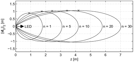
Figure 3: RSS contours for a given LED mode. All the locations on the RSS contours have identical RSS values.

$$\begin{bmatrix}\frac{\partial{P_{mk}}}{\partial{a}_{mk}}\\ \frac{\partial{P_{mk}}}{\partial{b}_{mk}}\\ \frac{\partial{P_{mk}}}{\partial{c}_{mk}}\\ \end{bmatrix}^{\rm T}\textrm{=}\begin{bmatrix}\textrm{-}\frac{(n+1)A_{\rm R}}{2\pi}{\Pi}\left(\frac{\theta_{mk}}{\theta_{\rm FOV}}\right){\Pi}\left(\frac{\phi_{mk}}{\pi/2}\right)g\left({a}_{mk};{n}_{{mk}}^{(x)},{n}_{{\rm R}}^{(x)},{b}_{mk}{n}_{{mk}}^{(y)}\textrm{+}{c}_{mk}{n}_{{mk}}^{(z)},{b}_{mk}{n}_{{\rm R}}^{(y)}\textrm{+}{c}_{mk}{n}_{{\rm R}}^{(z)},{b}_{mk}^{2}\textrm{+}{c}_{mk}^{2},n\right)\\ \textrm{-}\frac{(n+1)A_{\rm R}}{2\pi}{\Pi}\left(\frac{\theta_{mk}}{\theta_{\rm FOV}}\right){\Pi}\left(\frac{\phi_{mk}}{\pi/2}\right)g\left({b}_{mk};{n}_{{mk}}^{(y)},{n}_{{\rm R}}^{(y)},{a}_{mk}{n}_{{mk}}^{(x)}\textrm{+}{c}_{mk}{n}_{{mk}}^{(z)},{a}_{mk}{n}_{{\rm R}}^{(x)}\textrm{+}{c}_{mk}{n}_{{\rm R}}^{(z)},{a}_{mk}^{2}\textrm{+}{c}_{mk}^{2},n\right)\\ \textrm{-}\frac{(n+1)A_{\rm R}}{2\pi}{\Pi}\left(\frac{\theta_{mk}}{\theta_{\rm FOV}}\right){\Pi}\left(\frac{\phi_{mk}}{\pi/2}\right)g\left({c}_{mk};{n}_{{mk}}^{(z)},{n}_{{\rm R}}^{(z)},{a}_{mk}{n}_{{mk}}^{(x)}\textrm{+}{b}_{mk}{n}_{{mk}}^{(y)},{a}_{mk}{n}_{{\rm R}}^{(x)}\textrm{+}{b}_{mk}{n}_{{\rm R}}^{(y)},{a}_{mk}^{2}\textrm{+}{b}_{mk}^{2},n\right)\\ \end{bmatrix}^{\rm T}$$ (29)

The problem given in (12) corresponds to an unconstrained quadratic optimization problem, which can be solved via LS method. The closed-form solution of (12) can then be obtained as

$$\tilde{{\rm\bf r}}_{\rm R} ={{\rm\bf A}_{\rm w}}^{\rm\dagger}{\rm\bf b}_{\rm w}~{},$$ (19)

where $\displaystyle{\rm\bf A}_{{\rm w}}=\sum_{\begin{subarray}{c}k=1\\ m=s_{k}\end{subarray}}^{K}{P_{mk}}{\rm\bf A}_{mk}$ and $\displaystyle{\rm\bf b}_{\rm w}=\sum_{\begin{subarray}{c}k=1\\ m=s_{k}\end{subarray}}^{K}{P_{mk}}{\rm\bf b}_{mk}$.

IV RSS-Based Localization

Under the assumption of availability of physical characteristics of LEDs, the receiver can locate its own location based on RSS information associated with LED transmitters. Let ${\rm\bf s}\in\mathbb{R}^{MK\times 1}$ be the observation vector which is given by

$${\rm\bf s}={{\rm\bf p}({\bm{\uptheta}})}+{\rm\bf n}~{},$$ (20)

where ${\rm\bf n}\in\mathbb{R}^{KM\times 1}\sim\mathcal{N}\left(0,\sigma_{\rm n}^{2}{\rm\bf I}_{KM}\right)$ is an additive Gaussian noise vector, ${{\rm\bf p}({\bm{\uptheta}})}={\rm vec}\left({\rm\bf P({\bm{\uptheta}})}\right)\in\mathbb{R}^{MK\times 1}$, and ${\rm\bf P({\bm{\uptheta}})}\in\mathbb{R}^{M\times K}$ is a matrix which contains the exact RSS information with the entry on $m$th row and $k$th column being ${P_{mk}}$. The log-likelihood function for the location of VLC receiver is then expressed as

$$\mathcal{L}\left({\bm{\uptheta}}\right)=\log p\left({\rm\bf s};{\bm{\uptheta}}\right)~{},$$ (21)

where

$$p\left({\rm\bf s};{\bm{\uptheta}}\right)=\frac{1}{2\pi\sigma_{\rm n}^{2}}\exp{\left(-\frac{1}{2\sigma_{\rm n}^{2}}({\rm\bf s}-{{\rm\bf p}({\bm{\uptheta}})})^{\rm T}({\rm\bf s}-{{\rm\bf p}({\bm{\uptheta}})})\right)}$$ (22)

and ${\bm{\uptheta}}\in\mathbb{R}^{3\times 1}$ is the parameter vector which corresponds to the location of the VLC receiver, i.e., ${\rm\bf r}_{\rm R}$. Maximum likelihood (ML) estimate of ${\rm\bf r}_{\rm R}$ is therefore formulated as

$$\tilde{{\rm\bf r}}_{\rm R} =\arg\max_{{\bm{\uptheta}}}\mathcal{L}\left({\bm{\uptheta}}\right)\propto\arg\max_{{\bm{\uptheta}}}{\left(-({\rm\bf s}-{{\rm\bf p}({\bm{\uptheta}})})^{\rm T}({\rm\bf s}-{{\rm\bf p}({\bm{\uptheta}})})\right)}~{}.$$ (23)

As a result, (23) can be expressed as a nonlinear least squares (NLS) problem given by

$$\tilde{{\rm\bf r}}_{\rm R}=\arg\min_{{\bm{\uptheta}}}{\left(\lVert{{\rm\bf s}-{{{\rm\bf p}({\bm{\uptheta}})}}}\rVert_{2}^{2}\right)}~{}.$$ (24)

In the following subsections, first, we introduce a learning rule in order to solve (24). We then investigate the non-convex structure of (24) and address the initialization issues of the learning rule via the RRC algorithm. Finally, we provide CRLB of (24).

IV-A Learning Rule for RSS-Based Localization

In order to solve the system of nonlinear equations in (24), we follow multivariate Newton-Raphson method, which yields

$${\bm{\uptheta}}^{i+1}={\bm{\uptheta}}^{i}-\eta{\rm\bf H}^{\dagger}({\rm\bf s}-{{\rm\bf p}({\bm{\uptheta}}^{i})})~{},$$ (25)

where $\eta\in(0,1]$ is the step size and ${\rm\bf H}$ is the Jacobian matrix of ${{\rm\bf p}({\bm{\uptheta}})}$ with respect to ${\bm{\uptheta}}$. As $\theta_{1}$, $\theta_{2}$, and $\theta_{3}$ corresponds to $x$, $y$, and $z$ in (20), respectively, ${\rm\bf H}$ can be explicitly given by

$${\rm\bf H}=\begin{bmatrix}\frac{\partial{P_{00}}}{\partial x}&\frac{\partial{P_{00}}}{\partial y}&\frac{\partial{P_{00}}}{\partial z}\\ \frac{\partial{P_{10}}}{\partial x}&\frac{\partial{P_{10}}}{\partial y}&\frac{\partial{P_{10}}}{\partial z}\\ \vdots&\vdots&\vdots\\ \frac{\partial{P_{MK}}}{\partial x}&\frac{\partial{P_{MK}}}{\partial y}&\frac{\partial{P_{MK}}}{\partial z}\\ \end{bmatrix}~{}.$$ (26)

As it can be seen in (26), each row of ${\rm\bf H}$ indicates how the RSS associated with an LED transmitter change when the receiver moves in one of the axes, i.e., $x$, $y$, and $z$. Considering the chain rule of derivatives, the row associated with the $m$th LED transmitter of $k$th VAP is calculated as

$$\begin{bmatrix}\frac{\partial{P_{mk}}}{\partial x}\\ \frac{\partial{P_{mk}}}{\partial y}\\ \frac{\partial{P_{mk}}}{\partial z}\\ \end{bmatrix}^{\rm T}=\begin{bmatrix}\frac{\partial{P_{mk}}}{\partial{a}_{mk}}\\ \frac{\partial{P_{mk}}}{\partial{b}_{mk}}\\ \frac{\partial{P_{mk}}}{\partial{c}_{mk}}\\ \end{bmatrix}^{\rm T}\begin{bmatrix}\frac{\partial{a}_{mk}}{\partial x}&\frac{\partial{a}_{mk}}{\partial y}&\frac{\partial{a}_{mk}}{\partial z}\\ \frac{\partial{b}_{mk}}{\partial x}&\frac{\partial{b}_{mk}}{\partial y}&\frac{\partial{b}_{mk}}{\partial z}\\ \frac{\partial{c}_{mk}}{\partial x}&\frac{\partial{c}_{mk}}{\partial y}&\frac{\partial{c}_{mk}}{\partial z}\\ \end{bmatrix}~{}.$$ (27)

Since ${\rm\bf v}_{mk}={\rm\bf r}_{\rm R}-{\rm\bf r}_{mk}$, the matrix in (27), i.e., Jacobian of ${\rm\bf v}_{mk}$ respect to ${\bm{\uptheta}}$, becomes an identity matrix. Therefore, (27) can be directly calculated by evaluating the derivative of ${P_{mk}}$ with respect to ${\rm\bf v}_{mk}$ at ${\rm\bf v}_{mk}={\rm\bf r}_{\rm R}-{\rm\bf r}_{mk}$. The derivative of ${P_{mk}}$ with respect to ${\rm\bf v}_{mk}$ is analytically given in (29) by employing an auxiliary function $g\left(x;a,b,k,l,m,n\right)$ defined as

$$g\left(x;a,b,k,l,m,n\right) \triangleq\frac{\partial f\left(x;a,b,k,l,m,n\right)}{\partial x}$$

$$= \frac{(ax+k)^{(n-1)}(c_{3}x^{3}+c_{2}x^{2}+c_{1}x+c_{0})}{(x^{2}+m)^{\frac{n+5}{2}}}~{},$$

where $f\left(x;a,b,k,l,m,n\right)$ is a function based on the structure of ${P_{mk}}$ and keeping one of the elements of incidence vector ${\rm\bf v}_{mk}$ as a variable and the others as constants in (7). It is explicitly defined as

$$f\left(x;a,b,k,l,m,n\right)\triangleq\frac{(ax+k)^{(n-1)}(bx+l)}{(x^{2}+m)^{\frac{n+3}{2}}},$$ (28)

where $c_{0}=kbm+lamn$, $c_{1}=bmna+bma-lk(n+3)$, $c_{2}=-(kb(n+2)+3la)$, and $c_{3}=-2ab$. After plugging ${\rm\bf v}_{mk}={\rm\bf r}_{\rm R}-{\rm\bf r}_{mk}$ into (29), i.e., ${a}_{mk}=x-x_{mk}$, ${b}_{mk}=y-y_{mk}$, and ${c}_{mk}=z-z_{mk}$, (26) and (27) are obtained theoretically. Therefore, the learning rule given in (25) can be calculated analytically, which eliminates the numerical calculation of ${\rm\bf H}$ and yields less complex structures.

IV-B Non-Convex Structure of RSS-Based Localization

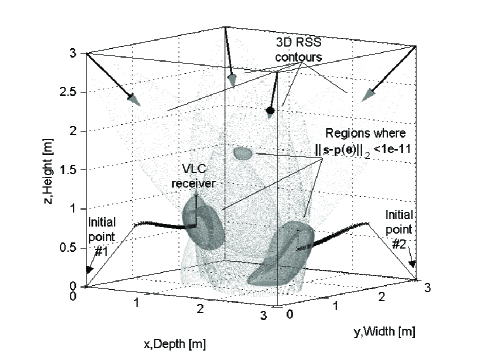
Figure 4: Convexity of (24). In this setup, there are three regions where the modeling error is less than $1$e-$11$ and lead to three different local optimum points which indicate non-convex structure of (24). While the first initial point allows (25) to find the global optimum, i.e., receiver’s location, the second initial point converges to one of the local optima.

Although Lambertian pattern offers a convex set by itself, (24) is not a convex function in general. This is due to the fact that the set of feasible solutions associated with each LED transmitter may become closer to each other in multiple locations in 3D geometry. For instance, consider a $3$ m $\times$ $3$ m $\times$ $3$ m where the VAPs are located at the corners as illustrated in Figure 4. In this setup, we assume that each VAP has single LED transmitter where $n=30$ and the angles between LED directions and side walls are set to $45$ degrees. The VLC receiver parameters are set as $\theta_{\rm FOV}=85$ degrees, $A_{\rm R}=1$ cm², ${\rm\bf r}_{\rm R}=[1,1,0.75]^{\rm T}$, and ${\rm\bf n}_{\rm R}=[0,0,1]^{\rm T}$. Having individual RSS information from each LED transmitter based on (1), we then find the locations where VLC receiver could observe the same RSS information for each LED transmitter in 3D geometry, which corresponds to RSS contours.

As it can been seen in Figure 4, the VLC receiver is located at the intersection of RSS contours. However, there are other locations in the room where the RSS contours get closer to each other. When we evaluate (24) and find the locations where the modeling error, i.e., $\lVert{{\rm\bf s}-{{{\rm\bf p}({\bm{\uptheta}})}}}\rVert_{2}$, is less than $1$e-$11$, we observe three different regions which indicate at least three different local optimum points. Therefore, different initial points for the learning rule given in (25) may converge to different location estimates. For example, in Figure 4, while the first initial point yields the true location of the VLC receiver, the second one converges to one of the local optima, i.e., the point where the RSS contours get closer to each other.

IV-C Initialization of RSS-Based Localization

In order to increase the likelihood that (25) converges to the global optimum, one may use the solution of AOA-based localization method as an initial point. The AOA-based solution is useful, such that it provides a closed-form solution that is close to the exact location of the VLC receiver, and hence does not require exhaustive search methods. However, this method may still lead to wrong results in some cases. In order to identify better initial points which increase the likelihood of finding the global optimum, i.e., location of the receiver, we propose a heuristic algorithm which is based on random search [23] and unsupervised clustering methods [24], which we call as the RRC algorithm.

RRC algorithm includes two steps: 1) random reporting and 2) clustering. In the first step, the algorithm generates $S$ random location samples in 3D space. The rewards achieved by the location samples are then calculated based on the modeling error in (21). By evaluating the rewards, only $G<S$ points that give the most promising results are chosen and the rest of the sample locations are eliminated. If the solution space is sampled in a sufficiently dense way, the favorable location samples should be located in the space as clusters since the objective function is non-convex and local regions appear in 3D space as clusters as illustrated in Figure 4.

In the second step, we aim at finding the centroids of the clusters. The reason for finding the centroids is that they are more likely to be around the true location of the VLC receiver, which make them good candidates for the initial points. To this end, we exploit unsupervised learning methods which are well investigated in the machine learning literature. Due to its simplicity, in this study, we employ $K$-means algorithm which is an effective method for finding the centroids of the clusters in a high-dimensional space [24, 25, 26]. Essentially, $K$-means algorithm converges to the centroids of the clusters with iterations. It applies two steps per each iteration. In the first step of $j$th iteration of $K$-means algorithm, the points are partitioned into $C$ clusters, $\{R_{\it i=1}^{j},R_{\it i=2}^{j},\dots,R_{\it i=C}^{j}\}$, based on their distances to the centroids obtained in $(j-1)$th iteration. In the second step, the $i$th centroid, i.e., ${\rm\bf c}_{i}$, is updated to better fit for the location samples as

$${\rm\bf c}_{i}^{(j+1)}=\frac{1}{\left|{R_{\it i}^{(j)}}\right|}\sum_{\ell\in R_{\it i}^{(j)}}{\rm\bf p}_{\ell}~{},$$ (29)

where ${\rm\bf p}_{\ell}$ is the $\ell$th point obtained from random reporting step and $\left|{\cdot}\right|$ is the cardinality of its argument. Once we obtain the centroids, we utilize them as initial points for the update rule in (25). We then select the best point based on (24).

IV-D Cramér-Rao Lower Bound for RSS-Based Localization

Without loss of generality, when ${\rm\bf x}\sim\mathcal{N}\left({\bm{\mu}}({\bm{\uptheta}}),{\rm\bf C}({\bm{\uptheta}})\right)$, the element on $i$th row and $j$th column of Fisher Information Matrix (FIM) ${\rm\bf J({{\bm{\uptheta}}})}$ can be calculated as [22]

$$[{\rm\bf J({{\bm{\uptheta}}})}]_{ij}= \left[\frac{\partial{\bm{\mu}}({\bm{\uptheta}})}{\partial\theta_{i}}\right]^{\rm T}{\rm\bf C}({\bm{\uptheta}})^{-1}\left[\frac{\partial{\bm{\mu}}({\bm{\uptheta}})}{\partial\theta_{j}}\right]$$

$$+\frac{1}{2}{\rm tr}\left[{\rm\bf C}({\bm{\uptheta}})^{-1}\frac{\partial{\rm\bf C}({\bm{\uptheta}})}{\partial\theta_{i}}{\rm\bf C}({\bm{\uptheta}})^{-1}\frac{\partial{\rm\bf C}({\bm{\uptheta}})}{\partial\theta_{j}}\right]~{}.$$ (30)

Since the noise term in (20) is assumed to be white Gaussian noise and does not depend on the location of receiver, the second term is zero and first term yields $[{\rm\bf J({{\bm{\uptheta}}})}]_{ij}=\frac{1}{\sigma_{\rm n}^{2}}\left[\frac{\partial{\bm{\mu}}({\bm{\uptheta}})}{\partial\theta_{i}}\right]^{\rm T}\left[\frac{\partial{\bm{\mu}}({\bm{\uptheta}})}{\partial\theta_{j}}\right]$. Based on (20), ${\bm{\mu}}({\bm{\uptheta}})$ corresponds to mean power captured power from all transmitters, i.e., ${\bm{\mu}}({\bm{\uptheta}})={{\rm\bf p}({\bm{\uptheta}})}$, which leads to the following expression:

$$[{\rm\bf J({{\bm{\uptheta}}})}]_{ij}= \frac{1}{\sigma_{\rm n}^{2}}\left[\frac{\partial{{\rm\bf p}({\bm{\uptheta}})}}{\partial\theta_{i}}\right]^{\rm T}\left[\frac{\partial{{\rm\bf p}({\bm{\uptheta}})}}{\partial\theta_{j}}\right]~{}.$$ (31)

By using (31), complete FIM can be then calculated as

$${\rm\bf J({{\bm{\uptheta}}})}= \frac{1}{\sigma_{\rm n}^{2}}{\rm\bf H}^{\rm T}{\rm\bf H}~{},$$ (32)

where ${\rm\bf H}$ is the Jacobian matrix of ${{\rm\bf p}({\bm{\uptheta}})}$ with respect to ${\bm{\uptheta}}$, which is already derived analytically by using (27) and (29). Once ${\rm\bf J({{\bm{\uptheta}}})}$ is calculated, CRLB for the receiver location in 3D geometry is obtained as

$${\rm RMSE}(x,y,z)\geq\sqrt{{\rm tr}({\rm\bf J}^{-1}({{\bm{\uptheta}}}))}~{},$$ (33)

where ${\rm RMSE}(x,y,z)$ is the root mean square error (RMSE) of the estimator given in (24). It is worth noting that the analytic expression of ${\rm\bf H}$ allows arbitrary scenarios in 3D coordinates, which generalizes the theoretical results provided in [18] where the angle between detector plane and floor plane is fixed to $0$ degrees.

V Numerical Results

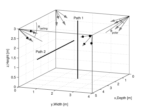
Figure 5: Simulation setup.

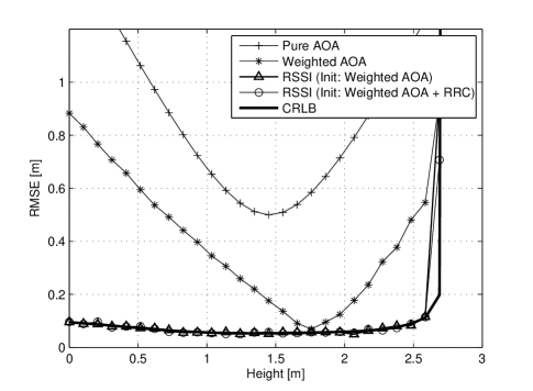
(a) Path 1, $n=10$.

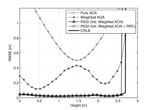
(b) Path 1, $n=30$.

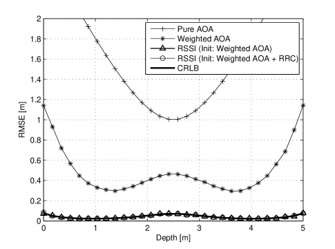
(c) Path 2, $n=10$.

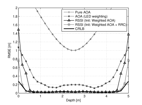
(d) Path 2, $n=30$.

Figure 6: Positioning accuracy on Path 1 and Path 2 ($\theta_{\rm polar}=20^{\circ}$, $\theta_{\rm ceiling}=30^{\circ}$).

In this section, we evaluate the performance of AOA and RSS based methods and impact of physical characteristics of LED transmitters on the estimators through computer simulations. For simulation tractability, we consider an empty room where its depth, width, and height are set to $5$, $4$, and $3$ meters, respectively. We deploy $4$ VAPs which are located at the corners of the room as shown in Figure 5. The angle between the direction of VAP and ceiling is denoted by $\theta_{\rm ceiling}$. Each VAP has $4$ LED transmitters where the angle between the direction of VAP and the direction of LED transmitters is assumed to be identical and parameterized as $\theta_{\rm polar}$. For the VLC receiver, $\theta_{\rm FOV}$ and $A_{\rm R}$ are set to $85$ degrees and $1$ cm², respectively. The direction of the VLC receiver is assumed to be ${\rm\bf n}_{\rm R}=[0,0,1]^{\rm T}$. Finally, based on the noise model given in [18] and the references therein, we set $\sigma_{\rm n}^{2}$ to $1$e$-13$ A².

V-A Performance of AOA and RSS Based Location Estimators

In order to evaluate the estimators discussed in Section III and Section IV numerically, we consider two different paths, i.e., Path 1 and Path 2, as shown in Figure 5. Path 1 considers a VLC receiver where its localization on x-axis and y-axis are fixed to $2$ m. On the other hand, Path 2 follows a horizontal path where the exact position of the VLC receiver on y-axis and z-axis are set to $1$ m and $1.5$ m, respectively. We then sweep the VLC receiver’s position on z-axis for Path 1 and x-axis for Path 2 and calculate RMSE of each estimator after $50$ realizations. We perform the simulations for $n=10$ and $n=30$ in (1) when $\theta_{\rm ceiling}=30^{\circ}$ and $\theta_{\rm polar}=20^{\circ}$.

As it can be seen from Figure 6, LED mode, i.e., $n$, does not affect the performance of pure AOA method based on (11) for both Path 1 and Path 2. This result is expected since the LED transmitters are assumed to be identical. Therefore VLC receiver selects the same LED transmitters as anchors regardless of $n$, which yields the same estimation results for pure AOA method. However, LED directivity, characterized by $n$, significantly affects the performance of AOA-based estimation, when RSS information is taken into account. For weighted AOA method based on (19), increasing $n$ provides better estimation results on both Path 1 and Path 2. This is due to the fact that RSS information becomes a dominant factor when VLC receiver is close to the line pointed by the orientation vectors of LED transmitters. In other words, nodes with higher $n$ have more reliable AOA estimates for a given RSS value, which is captured by the proposed weighted LS estimator.

For RSS-based localization, we consider two different initializations for the Newton-Raphson method ($\eta=0.2$) given in (25). We first run the simulations when weighted AOA results are considered as the initialization points. In this case, the search algorithm may happen to converge to local optima, which causes significant positioning errors. For example, the estimator performance degrades drastically for Path 2 when the VLC receiver is close to the side walls of the room, as given in Figure 6LABEL:sub@fig:path1n30. On the other hand, when RRC algorithm ($S=500$, $G=100$, and $C=4$) is applied for finding better initial points, RSS based localization is more likely to find the global optimum and attains the CRLB in most of the positions.

When the position of VLC receiver is close to the ceiling, all methods that use RSS fail as shown in Figure 6LABEL:sub@fig:path1n10 and Figure 6LABEL:sub@fig:path1n30. This is due to the large angle between receiver orientation vector and the incidence vector which reduces the effective area of PD. In particular, after certain height, FOV of VLC receiver does not allow the PD to capture any signal, which explains why CRLB goes to infinity.

V-B Number Of Clusters for RRC Algorithm

In this subsection, we evaluate the impact of number cluster of RRC algorithm, based on the configuration given in Figure 5. As a pessimistic scenario, we consider a VLC receiver located at the origin of the coordinate system. We then provide the probability of convergence to the location of VLC receiver for $C=\{0,1,2,3,4\}$ when $n=10$ and $n=30$. For each scenario, we also include the result of weighted AOA to the initial points obtained via RRC algorithm. In order to have a better understanding on the convergence, we evaluate the impact of number clusters in the noiseless case. We assume that a successful converge is considered when $\lVert{\tilde{{\rm\bf r}}_{\rm R}-{\rm\bf r}_{\rm R}}\rVert_{2}^{2}$ is less than $1$e$-2$.

As shown in Figure 7, increasing number of clusters yields better probability of converge. However, different LED modes require different number of clusters. For example, while RRC with $2$ clusters is sufficient to attain the global optimum with very high probability when $n=10$, RRC with $4$ cluster, i.e., 4 extra initial points beside weighted AOA result, yields high probability of convergence to global optimum when $n=30$.

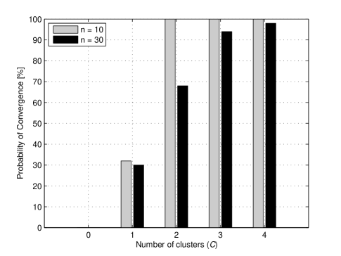
Figure 7: Probability of convergence for RRC algorithm.

V-C Configuration of VLC Access Points

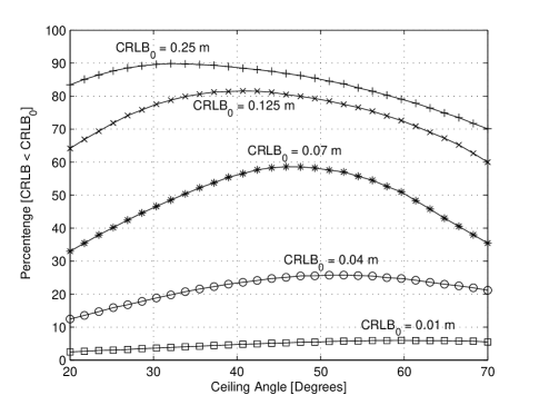
(a) $n=10$.

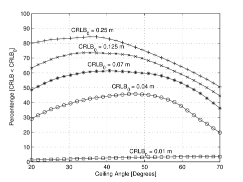
(b) $n=30$.

Figure 8: Probability of accuracy for a given $\theta_{\rm ceiling}$ ($\theta_{\rm polar}=20^{\circ}$).

In this subsection, we investigate the impact of deployment of VAP on positioning accuracy. We consider the simulation setup illustrated in Figure 5 and choose $\theta_{\rm ceiling}$ as a design parameter. We sweep $\theta_{\rm ceiling}$ between $20^{\circ}$ and $70^{\circ}$ and calculate CRLBs for the positions of the VLC receiver based on 3D grid in the whole room. We then calculate the probabilities where CRLB is less than or equal to certain values, i.e., ${\rm CRLB}_{0}=\{0.01,0.04,0.07,0.125,0.25\}$ in meters when $n=10$ and $n=30$. In the analysis, we fix $\theta_{\rm polar}$ to $20^{\circ}$.

As it can be seen from both Figure 8LABEL:sub@fig:n10 and Figure 8LABEL:sub@fig:n30, the optimum $\theta_{\rm ceiling}$ that gives the highest probability of accuracy in the room varies depending on $\rm CRLB_{0}$ and LED mode $n$. For example, the highest probability of accuracy is obtained at $\theta_{\rm ceiling}=60^{\circ}$ when $\rm CRLB_{0}=0.01$ m as given in Figure 8LABEL:sub@fig:n10. On the other hand, the highest probability is achieved at $\theta_{\rm ceiling}=30^{\circ}$ for the same LED mode when $\rm CRLB_{0}=0.25$ m. Similarly, when $n$ is set to $30$, the choice of $\theta_{\rm ceiling}=37^{\circ}$ yields the highest probability of accuracy for the same $\rm CRLB_{0}$ as given in Figure 8LABEL:sub@fig:n30.

It is also possible to infer how LED directivity affects the positioning accuracy overall in the room from Figure 8. As it can be seen from Figure 8LABEL:sub@fig:n10, $\%90$ of the room is covered when $\rm CRLB_{0}=0.25$ m and $n=10$. However, increasing LED mode $n$ to $30$ reduces the probability of accuracy to $\%85$ of the room as given in Figure 8LABEL:sub@fig:n30. On the other hand, higher LED mode increases the probability of highly accurate results. For example, when ${\rm CRLB}_{0}$ is fixed to $0.04$ m, $\%45$ of the room is covered for $n=30$ while it reduces to $\%27$ of the room for $n=10$.

V-D Orientations of LED Transmitters

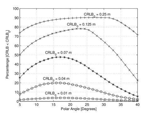
(a) $n=10$.

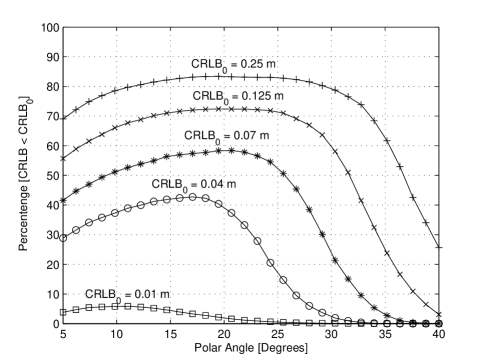
(b) $n=30$.

Figure 9: Probability of accuracy for a given $\theta_{\rm polar}$ ($\theta_{\rm ceiling}=30^{\circ}$).

In this subsection, we discuss the impact of the orientations of LED transmitters on positioning accuracy. Considering the setup illustrated in Figure 5, we sweep $\theta_{\rm polar}$ between $5^{\circ}$ and $40^{\circ}$. Similar to the analysis given in Section V-C, we obtain the probabilities that CRLB is less than or equal to certain values when $n=10$ and $n=30$. For this analysis, we fix $\theta_{\rm ceiling}$ to $30^{\circ}$.

As shown in Figure 9, the optimum $\theta_{\rm polar}$ depends on the LED mode and selected $\rm CRLB_{0}$. For instance, when $n=10$ and $\rm CRLB_{0}=0.01$ m, the optimum $\theta_{\rm polar}$ is $17.5^{\circ}$ as given in Figure 9LABEL:sub@fig:n10_polar. However, as shown in Figure 9LABEL:sub@fig:n30_polar, the optimum $\theta_{\rm polar}$ is obtained as $10^{\circ}$ when $n=30$. Similarly, when $\rm CRLB_{0}$ is set to $0.25$ m, $27^{\circ}$ and $19^{\circ}$ yield to the highest probability of accuracies in the room when $n=10$ and $n=30$, respectively. Nevertheless, in general, the optimum $\theta_{\rm polar}$ increases for higher ${\rm CRLB}_{0}$. This is due to the fact that larger $\theta_{\rm polar}$ yields more physical separation between LED transmitters for each VAP and the intensity distribution becomes more homogeneous in the room. Therefore while narrow $\theta_{\rm polar}$ yields more accurate results at specific points of the room, larger $\theta_{\rm polar}$ provides less accurate but better probability of accuracy for the setup given in Figure 5. On the other hand, increasing $\theta_{\rm polar}$ above the optimal point deteriorates the positioning accuracy as the orientations of LED transmitters start to be parallel to the walls of the room. In these cases, the center of the room does not receive sufficient amount of energy, which causes more positioning error.

VI Conclusion

In this study, we discuss AOA-based localization and RSS-based localization methods by considering hybrid utilization of AOA and RSS information in the location estimation. We show that AOA-based localization can be solved with an LS estimator. Yet its estimation results may be highly inaccurate, depending on the location of VLC receiver. On the other hand, when RSS information is utilized to weight LED transmitters in the optimization, the positioning accuracy increases significantly. For the scenario investigated in this study, i.e. a room with the dimensions of $3\times 5\times 4$ meters and $4$ VAPs, the localization error is less than $1$ meter. On the other hand, RSS-based localization method, which exploits the Lambertian patterns of LEDs, offers high positioning accuracy at the expense of a system of nonlinear equations and a non-convex objective function. In order to solve the system of nonlinear equations, we derive an analytical learning rule based on the Newton-Raphson method. Since the learning rule is analytical, it eliminates the calculation of Jacobian matrix numerically. For the hybrid utilization, the learning rule is initialized with the result of AOA-based method to increase the likelihood of converging to the global optimum, which the positioning accuracy improves up to $10$ cm. In addition to employing the results of AOA-based method, we also develop a heuristic search method, RRC algorithm, to identify extra initial points which could lead to find the global optimum.

In this investigation, we also discuss the impact of the orientations of LED transmitters and the physical characteristics of LEDs on the localization performance probabilistically. For this purpose, we utilize the CRLB that is derived for an arbitrary configuration in 3D geometry in this study. According to our analyses, when the illumination is homogeneous in 3D geometry, the positioning error becomes relatively high but mostly in attainable levels. On the other hand, when the illumination is not homogeneous due to the orientations of LEDs or using highly directive LEDs, the positioning accuracy is improved significantly at the locations where the energy is high; this also degrades the positioning accuracy at the same time in the locations where the energy, i.e., illumination, is low.

References

- [1] H. Liu, H. Darabi, P. Banerjee, and J. Liu, “Survey of wireless indoor positioning techniques and systems,” IEEE Trans. Syst., Man, Cybern.,Syst., vol. 37, no. 6, pp. 1067–1080, Nov. 2007.
- [2] D. Hahnel, W. Burgard, D. Fox, K. Fishkin, and M. Philipose, “Mapping and localization with RFID technology,” in Proc. IEEE Int. Conf. Robotics and Automation (ICRA), vol. 1, Apr. 2004, pp. 1015–1020.
- [3] M. Bouet and A. dos Santos, “RFID tags: Positioning principles and localization techniques,” in Proc. IEEE Wireless Days (WD), Nov. 2008, pp. 1–5.
- [4] B. Ciftler, A. Kadri, and I. Guvenc, “Fundamental bounds on RSS-based wireless localization in passive UHF RFID systems,” in Proc. IEEE Wireless Commun. Networking Conf., New Orleans, LO, Mar. 2015.
- [5] S. Gezici, Z. Tian, G. Giannakis, H. Kobayashi, A. Molisch, H. Poor, and Z. Sahinoglu, “Localization via ultra-wideband radios: a look at positioning aspects for future sensor networks,” IEEE Sig. Proc. Mag., vol. 22, no. 4, pp. 70–84, Jul. 2005.
- [6] A. Sayed, A. Tarighat, and N. Khajehnouri, “Network-based wireless location: challenges faced in developing techniques for accurate wireless location information,” IEEE Sig. Proc. Mag., vol. 22, no. 4, pp. 24–40, Jul. 2005.
- [7] I. Guvenc and C.-C. Chong, “A survey on TOA based wireless localization and NLOS mitigation techniques,” IEEE Commun. Surveys and Tutorials, vol. 11, no. 3, pp. 107–124, 2009.
- [8] K. Kaemarungsi, “Efficient design of indoor positioning systems based on location fingerprinting,” in Proc. IEEE Int. Conf. on Wireless Networks, Communications and Mobile Computing, vol. 1, Jun. 2005, pp. 181–186.
- [9] T. Komine and M. Nakagawa, “Fundamental analysis for visible-light communication system using LED lights,” IEEE Trans. Consum. Electron., vol. 50, no. 1, pp. 100–107, Feb. 2004.
- [10] A. Sevincer, A. Bhattarai, M. Bilgi, M. Yuksel, and N. Pala, “LIGHTNETs: smart lighting and mobile optical wireless networks – a survey,” IEEE Commun. Surveys and Tutorials, vol. 15, no. 4, pp. 1620–1641, Apr. 2013.
- [11] H. Burchardt, N. Serafimovski, D. Tsonev, S. Videv, and H. Haas, “VLC: Beyond point-to-point communication,” IEEE Commun. Mag., vol. 52, no. 7, pp. 98–105, Jul. 2014.
- [12] H. Elgala, R. Mesleh, and H. Haas, “Indoor optical wireless communication: potential and state-of-the-art,” IEEE Commun. Mag., vol. 49, no. 9, pp. 56–62, Sep. 2011.
- [13] J.-H. Liu, Q. Li, and X.-Y. Zhang, “Cellular coverage optimization for indoor visible light communication and illumination networks,” J. Commun., vol. 9, no. 11, Nov. 2014.
- [14] J. Kahn and J. Barry, “Wireless infrared communications,” Proc. IEEE, vol. 85, no. 2, pp. 265–298, Feb. 1997.
- [15] Y. S. Eroglu, I. Guvenc, N. Pala, and M. Yuksel, “AOA-based localization and tracking in multi-element VLC systems,” in Proc. IEEE Wireless and Microwave Technology Coneference (WAMICON), Coconut Beach, FL, Apr. 2015.
- [16] M. Bilgi, A. Sevincer, M. Yuksel, and N. Pala, “Optical wireless localization,” Wirel. Netw., vol. 18, no. 2, pp. 215–226, Feb. 2012.
- [17] Z. Zhou, M. Kavehrad, and D. Peng, “Indoor positioning algorithm using light-emitting diode visible light communications,” Optical Engineering, vol. 51, Aug. 2012.
- [18] X. Zhang, J. Duan, Y. Fu, and A. Shi, “Theoretical accuracy analysis of indoor visible light communication positioning system based on received signal strength indicator,” IEEE J. Lightw. Technol., vol. 32, no. 21, pp. 4180–4186, Nov. 2014.
- [19] J. Barry, J. Kahn, W. Krause, E. Lee, and D. Messerschmitt, “Simulation of multipath impulse response for indoor wireless optical channels,” IEEE J. Select. Areas Commun. (JSAC), vol. 11, no. 3, pp. 367–379, Apr. 1993.
- [20] M. Bilgi and M. Yuksel, “Capacity scaling in free-space-optical mobile ad hoc networks,” Ad Hoc Networks, vol. 12, pp. 150–164, 2014.
- [21] D. Tsonev, S. Videv, and H. Haas, “Light fidelity (Li-Fi): towards all-optical networking,” Proc. SPIE, vol. 9007, pp. 900 702–900 702–10, 2013.
- [22] S. M. Kay, Fundamentals of Statistical Signal Processing: Estimation Theory. Upper Saddle River, NJ, USA: Prentice-Hall, Inc., 1993.
- [23] T. Ye, H. Kaur, S. Kalyanaraman, and M. Yuksel, “Large-scale network parameter configuration using an on-line simulation framework,” IEEE/ACM Trans. Netw., vol. 16, no. 4, pp. 777–790, Aug. 2008.
- [24] T. Hastie, R. Tibshirani, and J. Friedman, The Elements of Statistical Learning, ser. Springer Series in Statistics. New York, NY, USA: Springer New York Inc., 2001.
- [25] M. Aharon, M. Elad, and A. Bruckstein, “K-SVD: An algorithm for designing overcomplete dictionaries for sparse representation,” IEEE Trans. Sig. Proc., vol. 54, no. 11, pp. 4311–4322, Nov. 2006.
- [26] A. Gersho and R. M. Gray, Vector Quantization and Signal Compression. Norwell, MA, USA: Kluwer Academic Publishers, 1991.