Optimal input signal distribution and per-sample mutual information for nondispersive nonlinear optical fiber channel at large SNR

Abstract

We consider a model nondispersive nonlinear optical fiber channel with additive white Gaussian noise at large $\mathrm{SNR}$ (signal-to-noise ratio) in the intermediate power region. Using Feynman path-integral technique we for the first time find the optimal input signal distribution maximizing the channel’s per-sample mutual information. The finding of the optimal input signal distribution allows us to improve previously known estimates for the channel capacity. The output signal entropy, conditional entropy, and per-sample mutual information are calculated for Gaussian, half-Gaussian and modified Gaussian input signal distributions. We explicitly show that in the intermediate power regime the per-sample mutual information for the optimal input signal distribution is greater than the per-sample mutual information for the Gaussian and half-Gaussian input signal distributions.

I Introduction.

The channel capacity $C$ introduced by Shannon in his seminal work [1] is related to the maximum amount of information that can be reliably transmitted over a noisy communication channel. Shannon calculated the capacity of the linear channel with additive white Gaussian noise (AWGN) and found the famous logarithmic dependence of the channel’s capacity on the signal power:

$$C\propto\log_{2}\left(1+\mathrm{SNR}\right)\,,$$ (1)

where $\mathrm{SNR}=P/N$ is the signal-to-noise power ratio, $P$ is the signal power, and $N$ is the noise power. This, in particular, means that when the noise power $N$ is fixed, in order to increase the capacity one has to increase the signal power $P$.

The interest in nonlinear communication channels has been increasing since the beginning of the 2000’s when fiber optics communication systems had to increase both bandwidth and system reach which required the use of ever higher optical power. Fiber optic nonlinear channels have been studied both analytically and numerically in numerous papers, see e.g. [2, 3, 4, 5, 6, 7, 8, 9] and references therein. The simplified model nondispersive nonlinear optical fiber channel was considered, e.g. in [10, 11, 12, 13, 14]. The investigation of nonlinear communication channels where transmission is affected and changed by the signal power is a difficult problem, especially at large $\mathrm{SNR}$ [6]. Analysis of the capacity of these channels is technically challenging and new techniques and methods are highly desirable to advance these studies [3, 13, 15, 16, 17]. In this work we consider a simplified model nonlinear channel with a limited range of practical applications. However, methods developed for and tested on such model channels might be useful for much more complex and challenging nonlinear fiber communication problems. We introduce here a new approach to the calculation of the conditional probability density function via the path-integral technique and demonstrate its application using considered model channel as a particular example.

The channel capacity $C$ is defined as the maximum of the mutual information $I_{P_{X}[X]}$ with respect to the probability density function $P_{X}[X]$ of the input signal $X$:

$$C=\max_{P_{X}[X]}I_{P_{X}[X]},$$ (2)

where the maximum value of $I_{P_{X}[X]}$ should be found subject to the condition of fixed average signal power:

$$P=\int{\cal D}X|X|^{2}P_{X}[X].$$ (3)

The mutual information of a memoryless channel is defined in terms of the output signal entropy $H[Y]$ and conditional entropy $H[Y|X]$:

$$I_{P_{X}[X]}=H[Y]-H[Y|X],$$ (4)

with

$$\!\!\!H[Y|X] = -\int{\cal D}X{\cal D}YP_{X}[X]{P[Y|X]}\log P[Y|X],$$ (5)

$$\!\!\!H[Y] = -\int{\cal D}YP_{out}[Y]\log P_{out}[Y],$$ (6)

$$\!\!\!P_{out}[Y] = \int{\cal D}XP_{X}[X]P[Y|X],$$ (7)

where $P[Y|X]$ is the conditional probability density function (PDF) for an output signal $Y$ when the input signal is $X$, and $P_{out}[Y]$ is the PDF for an output signal $Y$. The measure ${\cal D}Y$ is defined as $\int{\cal D}YP[Y|X]=1$, and ${\cal D}X$ is defined as $\int{\cal D}XP_{X}[X]=1$. The capacity (2), as defined by (4)-(7), is measured in units of $(\log 2)^{-1}$ bits per symbol (also known as nats per symbol). The input and output signals are functions of time where the signal’s spectrum is restricted to a given bandwidth. In general, a sampling of the temporal signal should be introduced to define a discrete-time memoryless channel, however, here we consider only per-sample quantities.

The channel’s mutual information (4) depends on the probability distribution $P_{X}[X]$ of the input signal. The input signal PDF, that maximizes the channel’s per-sample mutual information is called “capacity-approaching” or “optimal” PDF $P_{X}^{opt}[X]$. Obviously, the problem of finding the optimal PDF of the input signal for nonlinear optical channels is of great practical importance.

In the previous studies of nondispersive nonlinear optical channels (e.g. [11], [13], [14]) the Gaussian and half-Gaussian input signal PDF’s were used as trial functions in order to put low bound constraint on the channel capacity, or to provide asymptotic estimate of the capacity in the regime of large SNR. The authors of [14] argued, that the half-Gaussian PDF which we denote as $P_{X}^{(1)}[X]$,

$$P_{X}^{(1)}[X]=\dfrac{\exp\left\{-|X|^{2}/(2{P})\right\}}{\pi|X|(2\pi{P})^{1/2}},\,$$ (8)

provides the best approximation for the “capacity-approaching” input signal distribution at large SNR. In the present paper by solving a variational problem we show that it is not the case. We find a true optimal distribution $P_{X}^{opt}[X]$ (which in fact is different from half-Gaussian distribution) in the regime of large SNR for intermediate power range. We explicitly show, that in this regime the mutual information (4) for our optimal input signal PDF is larger than the mutual information for the Gaussian and half-Gaussian input signal distributions.

The estimates for the capacity of nonlinear fiber channels with zero dispersion and additive white Gaussian noise in the regime of large SNR were obtained in Refs. [13], [14]. The lower bound for capacity of the channel, based on trial Gaussian input signal PDF, reads [13]:

$$C\geq\frac{1}{2}\log\left(\mathrm{SNR}\right)+\frac{1+\gamma_{E}-\log(4\pi)}{2}+{\cal O}\left(\frac{\log\left(\mathrm{SNR}\right)}{\mathrm{SNR}}\right)\,,$$ (9)

where $\gamma_{E}\approx 0.5772$ is the Euler constant. Note that the second term on the right-hand side of Eq. (9) was presented as ${\cal O}(1)$ in Ref. [13] but it is easily calculated using Eqs. (23) and (24) of Ref. [13]. The pre-logarithmic factor $1/2$ in Eq. (9) arises as a result of the fact that in the high power regime, when the signal power $P\gtrsim\Big{(}N\gamma^{2}L^{2}\Big{)}^{-1}$, the signal-dependent phase noise due to self phase modulation occupies the entire phase interval $[0,2\pi]$ and, as a result, the phase does not transfer information, see Ref. [14]. Here $\gamma$ is the Kerr nonlinearity coefficient and $L$ is the fiber link length, see below. In [14] capacity estimates were also given in the intermediate power range $N\ll P\ll 6\pi^{2}\Big{(}N\gamma^{2}L^{2}\Big{)}^{-1}$. For such a power $P$ the following estimate of the lower bound for the capacity, based on the half-Gaussian input signal PDF, was derived [14]:

$$C\geq-\log(\gamma NL)+\frac{\gamma_{E}-1+\log(3\pi)}{2}+{\cal O}\left(\frac{1}{\sqrt{\mathrm{SNR}}}\right),$$ (10)

where instead of ${\cal O}\left(\frac{1}{\sqrt{\mathrm{SNR}}}\right)$ the authors presented the explicit function of the parameter $\mathrm{SNR}$ which decreases at large $\mathrm{SNR}$, see Eq. (40) in [14]. However, the authors of [14] did not take into account the ${1}/{\sqrt{\mathrm{SNR}}}$ corrections in the output signal entropy $H[Y]$, therefore, using these explicit functions in the capacity inequality is beyond the calculation accuracy. It also means that the result Eq. (40) of [14] is not a lower bound on the capacity. It is worth noting that in their result there is term $\log 2$ missing. Also their result does not recover the Shannon limit $\log\,\mathrm{SNR}$ as $\gamma\to 0$. Moreover, it is strange that the capacity estimate goes to infinity when $\gamma$ tends to zero. Therefore, there are obvious flaws in the result (10).

The analytical expression for the conditional probability density function of the channel was obtained in the complex form of an infinite series [10, 13, 14] within the Martin-Siggia-Rose formalism based on quantum field theory methods [18]. In the present paper we adopt the Martin-Siggia-Rose formalism and develop a new method for the approximate computation of the conditional probability density function $P[Y|X]$. Using this method we obtain the simple analytical expression for the function $P[Y|X]$ in the leading and next-to-leading order in the parameter $1/\mathrm{SNR}$ for the intermediate power regime

$$N\ll P\ll\Big{(}N\gamma^{2}L^{2}\Big{)}^{-1}.$$ (11)

Our method allows us first to derive the analytical expression for the mutual information and then the optimal input signal distribution $P^{opt}_{X}[X]$ which is different from the half-Gaussian.

In [17] a method to calculate the conditional PDF for a nonlinear optical fiber channel with nonzero dispersion in the large $\mathrm{SNR}$ limit was introduced. Here we illustrate this general approach in application to a simpler nondispersive nonlinear optical fiber channel as considered in [13, 14, 10]. Since the channel is dispersionless, the temporal signal waveform does not change during propagation (note, though, that the signal bandwidth will grow due to the fiber nonlinearity and signal modulation). Therefore, instead of considering the evolution of $\psi(z,t)$ we can consider a set of independent scalar channels [10, 14] (per-sample channels) governed by the following model:

$$\partial_{z}\psi(z)-i\gamma|\psi(z)|^{2}\psi(z)=\eta(z),$$ (12)

where $\psi(z)$ is the signal function that is assumed to obey the boundary conditions $\psi(0)=X$, $\psi(L)=Y$. The noise $\eta(z)$ has zero mean $\langle\eta(z)\rangle_{\eta}=0$ and a correlation function $\langle\eta(z)\bar{\eta}(z^{\prime})\rangle_{\eta}=Q\delta(z-z^{\prime})\,$, so that the $\mathrm{SNR}=P/QL$, where $P$ and $N=QL$ are the per-sample signal power and the per-sample noise power, respectively. The connection between the differential model (12) and the conventional information-theoretic presentation in the form of an explicit input-output probabilistic model and appropriate sampling has been discussed in detail in [13, 14, 10]. For this per-sample channel we calculate the conditional probability density function (in order to illustrate how our method works), the conditional entropy (5), the output signal entropy (6), and the mutual information (4). Solving a variational problem for the mutual information we find the optimal input signal distribution $P_{X}[X]$ maximizing the mutual information in the leading order in $1/\mathrm{SNR}$.

The paper is organized as follows. In Section II we develop the quasi-classical method for the calculation of the conditional PDF $P[Y|X]$ for arbitrary nonlinearity in the intermediate power regime (11) in the leading and next-to-leading order in $1/\mathrm{SNR}$. We find a simple representation for $P[Y|X]$ in this case. This allows us to calculate the output signal distribution $P_{out}[Y]$. The optimal signal distribution $P_{X}^{opt}[X]$ is found in Section III. Section IV is focused on the calculation and the comparison of the mutual information for various input signal distributions. We demonstrate that there is a range of power $P$ where the mutual information $I_{P_{X}^{(2)}[X]}$ calculated for a Gaussian distribution $P_{X}^{(2)}[X]$, see Eq. (34) below, is closer to $I_{P_{X}^{opt}[X]}$, whereas at large enough power $P$ the mutual information $I_{P_{X}^{(1)}[X]}$ calculated for the half-Gaussian distribution $P_{X}^{(1)}[X]$ is closer to $I_{P_{X}^{opt}[X]}$ than the mutual information $I_{P_{X}^{(2)}[X]}$. We discuss our results in Section V.

II The conditional PDF $P[Y|X]$ and output signal PDF $P_{out}[Y]$ at large $\mathrm{SNR}$

II-A ”Quasiclassical” method for the conditional PDF $P[Y|X]$ calculation

The conditional probability density function can be written via the path-integral form [13, 18, 19] in a retarded discretization scheme, see e.g. Supplemental Materials of Ref. [17]

$$P[Y|X]=\!\!\!\!\int\limits_{\psi(0)=X}^{\psi(L)=Y}\!\!\!\!{\cal D}\psi\exp\Big{\{}-\frac{S[\psi]}{Q}\Big{\}}\,,$$ (13)

and can be reduced to the quasi-classical form, see Ref. [19]:

$$P[Y|X]=e^{-\frac{S[\Psi_{cl}(z)]}{Q}}\!\!\!\!\!\int\limits_{\tilde{\psi}(0)=0}^{\tilde{\psi}(L)=0}\!\!\!\!\!{\cal D}\tilde{\psi}\,e^{-\frac{S[\Psi_{cl}(z)+\tilde{\psi}(z)]-S[\Psi_{cl}(z)]}{Q}}\,,$$ (14)

where the effective action $S[\psi]=\int\limits_{0}^{L}dz\Big{|}\partial_{z}\psi-i\gamma|\psi|^{2}\psi\Big{|}^{2}$, and the function $\Psi_{cl}(z)$ is the ”classical” solution of the equation $\delta S[\Psi_{cl}]=0$, where $\delta S$ is the variation of our action $S[\psi]$. The equation $\delta S[\Psi_{cl}]=0$ (Euler-Lagrange equation) has the form

$$\frac{d^{2}\Psi_{cl}}{dz^{2}}-4i\gamma\left|\Psi_{cl}\right|^{2}\frac{d\Psi_{cl}}{dz}-3\gamma^{2}\left|\Psi_{cl}\right|^{4}\Psi_{cl}=0,$$ (15)

with the boundary conditions $\Psi_{cl}(0)=X$, $\Psi_{cl}(L)=Y$.

In order to find $P[Y|X]$ one should calculate the exponent $e^{-\frac{S[\Psi_{cl}(z)]}{Q}}$ and the path-integral in Eq. (14). First, we evaluate the exponent. To find it we have to calculate the function $\Psi_{cl}(z)$ and then the action $S[\Psi_{cl}(z)]$. We found the general solution $\Psi_{cl}(z)$ of (15) implicitly through the boundary conditions, see Eqs. (68)–(72), and Eq. (74) in Appendix -A. This form of the solution is inconvenient for further calculations. Therefore we adopt a different approach and find the solution in the leading and next-to-leading order in $1/\mathrm{SNR}$, linearizing Eq. (15) in the vicinity of the solution $\Psi_{0}(z)$. Here $\Psi_{0}(z)$ is the solution of the equation (12) with zero noise and with the boundary condition $\Psi_{0}(0)=X=\rho e^{i\phi^{(X)}}$. The function $\Psi_{0}(z)$ reads

$$\Psi_{0}(z)=\rho\exp\left\{i\mu\frac{z}{L}+i\phi^{(X)}\right\},$$ (16)

where $\mu=\gamma L\rho^{2}=\gamma L|X|^{2}$. Note that this solution satisfies only the input boundary condition $\Psi_{0}(0)=X=\rho e^{i\phi^{(X)}}$, and it is the solution of Eq. (15) as well. Therefore, we look for the solution of Eq. (15) in the following form

$$\Psi_{cl}(z)=\Big{(}\rho+\varkappa(z)\Big{)}\exp\left\{i\mu\frac{z}{L}+i\phi^{(X)}\right\},$$ (17)

where the function $\varkappa(z)$ is assumed to be small: $|\varkappa(z)|\ll\rho$. In the general case, the ratio $|\varkappa(z)|/\rho$ is not necessarily small and it depends on the output boundary condition $\varkappa(L)$. However, the configurations of $\varkappa(z)$ at which $\Psi_{cl}(z)$ significantly deviates from $\Psi_{0}(z)$ ($|\varkappa(z)|\sim\rho$) are statistically irrelevant. Indeed, the expansion $S[\Psi_{0}(z)+\delta\Psi(z)]\propto\varkappa^{2}(z)$ starts from the quadratic term at small $\varkappa(z)$, since the action achieves an extremum (the absolute minimum $S[\Psi_{0}(z)]=0$) on the solution $\Psi_{0}(z)$. Thus the exponent $e^{-\frac{S[\Psi_{cl}(z)]}{Q}}$ and, as a result, the conditional PDF $P[Y|X]$ vanishes exponentially if the typical $\varkappa(z)$ is much greater than $\sqrt{QL}$.

Substituting Eq. (17) into Eq. (15) and retaining only terms linear in $\varkappa(z)/\rho$, we obtain the following equation which is still exact in the non-linearity parameter $\mu$:

$$\frac{d^{2}\varkappa}{dz^{2}}-2i\frac{\mu}{L}\frac{d\varkappa}{dz}-4\frac{\mu^{2}}{L^{2}}Re[\varkappa]=0.$$ (18)

The boundary conditions for the function $\varkappa(z)$ read

$$\varkappa(0)=0,\,\varkappa(L)=Ye^{-i\phi^{(X)}-i\mu}-\rho\equiv x_{0}+iy_{0},$$ (19)

where $x_{0}=Re\{\varkappa(L)\}$ and $y_{0}=Im\{\varkappa(L)\}$. The solution of the linearized boundary problem (18), (19) reads

$$Re[\varkappa(z)]=\Big{(}\mu\frac{\mu x_{0}-y_{0}}{1+\mu^{2}/3}\frac{z}{L}+\frac{(1-2\mu^{2}/3)x_{0}+\mu y_{0}}{1+\mu^{2}/3}\Big{)}\frac{z}{L},$$

$$Im[\varkappa(z)]=\Big{(}\frac{\mu x_{0}-y_{0}}{1+\mu^{2}/3}\left(\frac{2\mu^{2}z^{2}}{3L^{2}}-1\right)+\mu\,\frac{(1-2\mu^{2}/3)x_{0}+\mu y_{0}}{1+\mu^{2}/3}\frac{z}{L}\Big{)}\frac{z}{L}.$$ (20)

After substitution of the solution Eq. (II-A) in the action we obtain

$$\frac{1}{Q}S[\Psi_{cl}(z)]=\frac{1}{Q}S\left[\left(\rho+\varkappa(z)\right)\exp\left\{i\mu\frac{z}{L}+i\phi^{(X)}\right\}\right]\approx$$

$$\frac{1}{Q}\int^{L}_{0}dz\Big{|}\partial_{z}\varkappa-2i\frac{\mu}{L}Re[\varkappa]\Big{|}^{2}=$$

$$\frac{(1+4\mu^{2}/3)x^{2}_{0}-2\mu x_{0}y_{0}+y^{2}_{0}}{QL(1+\mu^{2}/3)}.$$ (21)

Note that here we retain only the terms quadratic in $\varkappa$. However, it is straightforward to calculate the next correction to the action (II-A) which is $O(1/\sqrt{\mathrm{SNR}})$, see details in Appendix -A. A regular perturbative expansion for $\varkappa(z)$ in powers of $1/\sqrt{\mathrm{SNR}}$ can be obtained using the exact equation for the function $\varkappa(z)$, see Eq. (-A) in Appendix -A.

The next step in evaluation of the conditional probability $P[Y|X]$ is the calculation of the path-integral in Eq. (14). In order to calculate the path-integral in the leading $1/\mathrm{SNR}$ order we retain only quadratic in $\tilde{\psi}$ terms in the integrand. Any extra power of $\tilde{\psi}$ or $\varkappa$ is suppressed by the multiplicative parameter $\sqrt{QL}$, because at small $Q$ the main contribution to the path-integral comes from $\tilde{\psi}\sim\sqrt{QL}$. Moreover, as soon as we calculate the path-integral in the leading order in $Q$, we can substitute $\Psi_{0}(z)$ for $\Psi_{cl}(z)$ in the action difference $S[\Psi_{cl}(z)+\tilde{\psi}(z)]-S[\Psi_{cl}(z)]$. To find $P[Y|X]$ in the next-to-leading order in $1/\mathrm{SNR}$ we should retain both $\varkappa(z)$ in $\Psi_{cl}(z)$ and higher powers of $\tilde{\psi}$ in the action difference. Details of the path-integral calculation in the leading and next-to-leading order in $1/\sqrt{\mathrm{SNR}}$ are presented in Appendix -B. Taking into account the expression for the action (88) and the result of the path-integral calculation (-B) we obtain the final result for $P[Y|X]$:

$$\!\!\!P[Y|X]=\dfrac{\exp\left\{-\dfrac{(1+4\mu^{2}/3)x^{2}_{0}-2\mu x_{0}y_{0}+y^{2}_{0}}{QL(1+\mu^{2}/3)}\right\}}{\pi QL\sqrt{1+\mu^{2}/3}}\Bigg{(}1-\frac{\mu/\rho}{15(1+\mu^{2}/3)^{2}}\left(\mu(15+\mu^{2})x_{0}-2(5-\mu^{2}/3)y_{0}\right)-$$

$$\frac{\mu/\rho}{135QL\left(1+\mu^{2}/3\right)^{3}}\Big{\{}\mu\left(4\mu^{4}+15\mu^{2}+225\right)x^{3}_{0}+\left(23\mu^{4}+255\mu^{2}-90\right)x^{2}_{0}y_{0}+\mu\left(20\mu^{4}+117\mu^{2}-45\right)x_{0}y^{2}_{0}-$$

$$3\left(5\mu^{4}+33\mu^{2}+30\right)y^{3}_{0}\Big{\}}+{\cal O}\left(\frac{QL}{|X|^{2}}\right)+{\cal O}\left(\gamma^{2}L^{3}Q|X|^{2}\right)\Bigg{)},$$ (22)

where $x_{0}$ and $y_{0}$ are the functions of $X$ and $Y$ defined in (19). Since we consider here only the result (II-A) for the large $\mathrm{SNR}$ limit we imply that $|X|^{2}\gg QL$. Note that the conditional PDF $P[Y|X]$ was already derived in [13] in the form of an infinite series. Our result (II-A) for the function $P[Y|X]$ is the analytic summation of this series in the limit of large $\mathrm{SNR}$ and intermediate power region

$$QL\ll P\ll\left(QL^{3}\gamma^{2}\right)^{-1}.$$ (23)

The accuracy ${\cal O}\left(\gamma^{2}L^{3}Q|X|^{2}\right)$ in Eq. (II-A) appears in the calculation of the path-integral as a result of neglecting higher powers of the field $\tilde{\psi}$, see Eq. (-B) in Appendix -B. One can show that the normalization condition $\int DYP[Y|X]=1$ is fulfilled. Also one can check that the distribution (II-A) obeys the following important property

$$\lim_{Q\rightarrow 0}P[Y|X]=\delta\Big{(}Y-\Psi_{0}(L)\Big{)}.$$ (24)

The expression (24) is nothing else, but the deterministic limit of $P[Y|X]$ in the absence of noise. Also Eq. (II-A) has the correct limit for the linear channel ($\gamma\to 0$):

$$P^{(0)}[Y|X]=\frac{e^{-|Y-X|^{2}/{QL}}}{\pi QL}\,,$$ (25)

that is nothing else but the conditional PDF for the linear nondispersive channel with AWGN.

II-B Output signal PDF $P_{out}[Y]$

Now we proceed to calculate the probability density function of the output signal $P_{out}[Y]$. Let us consider the integral, see Eq. (7),

$$P_{out}[Y]=\int{\cal D}XP[Y|X]P_{X}[X],$$ (26)

where the function $P_{X}[X]$ is a smooth function with a scale of variation $P$ which is much greater than $QL$. In that case we can calculate the integral (26) with accuracies ${\cal O}\left({1}/{{\mathrm{SNR}}}\right)$ and ${\cal O}\left(\gamma^{2}L^{3}QP\right)$ by Laplace’s method [20], see Appendix -C. The result has the form:

$$P_{out}[Y]=\int{\cal D}XP[Y|X]P_{X}[X]=P_{X}\left[Ye^{-i\gamma|Y|^{2}L}\right]\left(1+{\cal O}\left({1}/{{\mathrm{SNR}}}\right)+{\cal O}\left(\gamma^{2}L^{3}QP\right)\right).$$ (27)

The main term of this result (27) can be easily obtained from the following reasoning. The function $P[Y|X]$, see Eq. (II-A), varies on a scale of order $QL$ which is much less than the scale of $P_{X}[X]$ (the function $P[Y|X]$ is essentially narrower than the function $P_{X}[X]$). Also $P[Y|X]$ has the delta-function limit (24) and therefore in the integral (26) it can be replaced with the delta-function. Note that to obtain the result (27) we do not require the limit $Q\rightarrow 0$ but only the relation between the scales ${P}$ and $QL$ to be satisfied. In what follows we will omit the terms ${\cal O}(\ldots)$ for brevity and restore them in the final results. For the case of the distribution $P_{X}[X]$ which depends only on $|X|$ we have $P_{out}[Y]=P_{X}[|Y|]$. For such distributions we can calculate corrections to (27) in the parameter $QL$ in any order in $QL$.

Let us restrict our consideration in the remainder of this Section to the distributions $P_{X}[X]$ depending only on $|X|$. We can use the $P[Y|X]$ found in Ref. [13], see Eqs. (11)–(13) therein. In this case $P_{out}[Y]$ is a function of $|Y|=\rho^{\prime}$

$${P}_{out}[\rho^{\prime}]=\dfrac{2e^{-\dfrac{\rho^{\prime 2}}{QL}}}{QL}\int^{\infty}_{0}d\rho\rho e^{-\dfrac{\rho^{2}}{QL}}I_{0}\left(\frac{2\rho\rho^{\prime}}{QL}\right){P}_{X}[\rho],$$ (28)

where $I_{0}(z)$ is the modified Bessel function of the first kind. Using this representation we can obtain the simple relation for ${P}_{out}[\rho^{\prime}]$ calculation in the perturbation theory in $QL$. To this end we perform the zero order Hankel transformation [20]:

$$\hat{P}[k]=\int^{\infty}_{0}d\rho\rho J_{0}(k\rho)P_{X}[\rho].$$ (29)

of both sides of Eq. (28), then we use the standard integral [21] with Bessel and modified Bessel functions

$$\int^{\infty}_{0}dzze^{-pz^{2}}J_{\nu}\left(bz\right)I_{\nu}(cz)=\frac{1}{2p}J_{\nu}\left(\frac{bc}{2p}\right)e^{\frac{c^{2}-b^{2}}{4p}},$$

and arrive at the simple relation between the Hankel images

$$\hat{P}_{out}[k]=e^{-k^{2}\frac{QL}{4}}\hat{P}[k].$$ (30)

Performing the inverse Hankel transformation

$${P}_{X}[\rho]=\int^{\infty}_{0}dkkJ_{0}(k\rho)\hat{P}[k],$$ (31)

we obtain

$${P}_{out}[\rho]=e^{\frac{QL}{4}\Delta_{\rho}}{P}_{X}[\rho],$$ (32)

where $\Delta_{\rho}=\frac{d^{2}}{d\rho^{2}}+\frac{1}{\rho}\frac{d}{d\rho}$ is the two-dimensional radial Laplace operator. From the relation (32) the problem of finding $(QL)^{n}$ corrections to ${P}_{out}[\rho]$ reduces to the exponent expansion and straightforward calculations of the action of the differential operator $\Delta_{\rho}^{n}$ on ${P}_{X}[\rho]$.

Let us consider the widely used example of the modified Gaussian distribution

$$P_{X}^{(\beta)}[\rho]=\frac{\exp\left\{-{\beta\rho^{2}}/{(2P)}\right\}\rho^{\beta-2}}{\pi\Gamma\left({\beta}/{2}\right)\left(2P/\beta\right)^{\beta/2}}.$$ (33)

For $\beta>0$ the distribution $P_{X}^{(\beta)}[\rho]$ is normalized to unity, $2\pi\int^{\infty}_{0}d\rho\rho P_{X}^{(\beta)}[\rho]=1$, and has the average power $P$, $2\pi\int^{\infty}_{0}d\rho\rho^{3}P_{X}^{(\beta)}[\rho]=P$. The distribution $P_{X}^{(\beta)}[X]$ generalizes the half-Gaussian distribution (8) for $\beta=1$ and the Gaussian for $\beta=2$:

$$P_{X}^{(2)}[X]=\frac{1}{\pi P}e^{-|X|^{2}/P}.$$ (34)

Inserting (34) into Eq. (28) we obtain a standard integral which can be found in [21]. The result for the output signal PDF has the form:

$$\!\!\!P_{out}^{(\beta)}[Y]=_{1}\!\!F_{1}\left(\frac{\beta}{2};1;\frac{|Y|^{2}2P}{QL(2P+\beta QL)}\right)\times$$

$$\frac{\exp\{-|Y|^{2}/QL\}}{\pi QL}\left(\frac{\beta QL}{2P+\beta QL}\right)^{\beta/2},$$ (35)

where ${}_{1}F_{1}(\frac{\beta}{2};1;z)$ is the confluent hypergeometric function that reduces to $e^{z}$ for the Gaussian case and to $e^{z/2}I_{0}(z/2)$ for the half-Gaussian case:

$$P_{out}^{(2)}[Y]=\frac{1}{\pi(P+QL)}\exp\left\{-\frac{|Y|^{2}}{P+QL}\right\},$$ (36)

$$P_{out}^{(1)}[Y]=\frac{\exp\{-|Y|^{2}/(2P+QL)\}}{\pi|Y|\sqrt{\pi(2P+QL)}}\times$$

$$\sqrt{\frac{\pi|Y|^{2}}{QL}}e^{-\frac{|Y|^{2}P}{QL(2P+QL)}}I_{0}\left(\!\!\frac{|Y|^{2}P}{QL(2P+QL)}\right).$$ (37)

Note that the result for $P_{out}^{(1)}[Y]$ in Ref. [14], see Eq. (38) therein, for the half-Gaussian distribution is incorrect. To demonstrate the general result of Eq. (27) let us consider Eq. (II-B) in the case $QL\ll|Y|^{2}\sim P$. For the case one can obtain:

$$P_{out}^{(1)}[Y]=P_{X}^{(1)}[|Y|]\left(1+{\cal O}\left(\frac{1}{\mathrm{SNR}}\right)\right).$$ (38)

The result (38) coincides with Eq.  (27) with the accuracy ${\cal O}\left(\gamma^{2}L^{3}QP\right)$.

III Optimal input signal distribution at large $\mathrm{SNR}$

The optimal input signal distribution at large $\mathrm{SNR}$ can be found calculating the mutual information (4) and then maximizing the result with respect to the input signal distribution function $P_{X}[X]$. Let us start from the calculation of the output signal entropy $H[Y]$, see Eq. (6), at large $\mathrm{SNR}$. When the parameter $\mathrm{SNR}\gg 1$ we can substitute $P_{X}\left[Y\exp\left\{-i\gamma|Y|^{2}L\right\}\right]$ instead of $P_{out}[Y]$ due to the relation (27):

$$H[Y] = -\int^{2\pi}_{0}d\phi\!\!\int^{\infty}_{0}d\rho^{\prime}\rho^{\prime}P_{X}\left[\rho^{\prime}e^{i\phi}\right]\times$$ (39)

$$\log P_{X}\left[\rho^{\prime}e^{i\phi}\right]+{\cal O}\left(\frac{1}{\mathrm{SNR}}\right)+{\cal O}\left(\gamma^{2}L^{3}QP\right).$$

In order to obtain Eq. (39) we have performed the change of the integration variable ${\phi}=\phi^{(Y)}+\gamma|Y|^{2}L$. One can see that the output signal entropy (39) coincides with the input signal entropy in the leading order in $1/\mathrm{SNR}$ and $\gamma^{2}L^{3}QP$.

The conditional entropy $H[Y|X]$ can be calculated by substitution of $P[Y|X]$ in the form of Eq. (II-A) into Eq. (5). After the substitution we change the integration variables ${\cal D}Y\equiv dReYdImY$ to $dx_{0}dy_{0}$. Then we perform integration over $x_{0}$, $y_{0}$ and obtain

$$\!\!\!\!\!\!\!\!\!\!\!\!H[Y|X]=1+\log({\pi QL})+$$

$$\!\!\!\!\!\!\!\!\!\!\!\!\frac{1}{2}\int^{2\pi}_{0}d\phi^{(X)}\int^{\infty}_{0}d\rho\rho P_{X}\left[\rho e^{i\phi^{(X)}}\right]\log\left(1+\frac{\gamma^{2}L^{2}}{3}\rho^{4}\right)+{\cal O}\left(\frac{1}{\mathrm{SNR}}\right)+{\cal O}\left(\gamma^{2}L^{3}QP\right),$$ (40)

where the first two terms come from the Gaussian type integrals over ${\cal D}Y$ in the conditional entropy definition (5) and the normalization factor $\pi QL$ in Eq. (II-A). The third term in Eq. (III) comes from the normalization factor $\sqrt{1+\mu^{2}/3}$, see Eq. (II-A). Note that there are no terms which are ${\cal O}\left({1}/\sqrt{\mathrm{SNR}}\right)$ in Eqs.  (39) and (III). Indeed, the integrals with the odd powers of $x_{0}$ and $y_{0}$ vanish when integrating over $x_{0}$, $y_{0}$ in Eq.  (5) for $H[Y|X]$.

To find the optimal distribution $P_{X}^{opt}[X]$ normalized to unity and having a fixed average power $P$ one should solve the variational problem for the functional $J[P_{X},\lambda_{1},\lambda_{2}]$

$$J[P_{X},\lambda_{1},\lambda_{2}]=H[Y]-H[Y|X]-\lambda_{1}\left(\int{\cal D}XP_{X}[X]-1\right)-$$

$$\lambda_{2}\left(\int{\cal D}XP_{X}[X]|X|^{2}-P\right),$$ (41)

where $\lambda_{1,2}$ are Lagrange multipliers. We substitute $H[Y]$ and $H[Y|X]$ from Eqs. (39) and (III) to (III), perform the variation of the functional $J[P_{X},\lambda_{1},\lambda_{2}]$ over $P_{X}[X]$, $\lambda_{1}$, $\lambda_{2}$, and write the Euler-Lagrange equations $\delta J[P_{X},\lambda_{1},\lambda_{2}]=0$:

$$\int{\cal D}XP_{X}[X]=1,$$ (42)

$$\int{\cal D}XP_{X}[X]|X|^{2}=P,$$ (43)

$$-1-\log P_{X}[X]-\frac{1}{2}\log\left(1+\frac{\gamma^{2}L^{2}}{3}|X|^{4}\right)-\lambda_{1}-\lambda_{2}|X|^{2}=0.$$ (44)

The solution $P_{X}^{opt}[X]$ of Eqs. (42)-(44) referred to as the “optimal” distribution depends only on $|X|$ and has the form:

$$P_{X}^{opt}[X]=N_{0}(P)\frac{\exp\left\{-\lambda_{0}(P)|X|^{2}\right\}}{\sqrt{1+\gamma^{2}L^{2}|X|^{4}/3}},$$ (45)

where functions $N_{0}(P)$ and $\lambda_{0}(P)$ are determined from the conditions  (42), (43):

$$\int{\cal D}XP_{X}^{opt}[X]=2\pi N_{0}(P)\int^{\infty}_{0}\frac{d\rho\,\rho\,e^{-\lambda_{0}(P)\rho^{2}}}{\sqrt{1+\gamma^{2}L^{2}\rho^{4}/3}}=1,$$ (46)

$$\!\!\int\!\!{\cal D}XP_{X}^{opt}[X]|X|^{2}\!\!=2\pi N_{0}(P)\!\!\int^{\infty}_{0}\!\!\frac{d\rho\,\rho^{3}\!e^{-\lambda_{0}(P)\rho^{2}}}{\sqrt{1+\gamma^{2}L^{2}\rho^{4}/3}}=P.$$ (47)

In a parametric form this dependance reads

$$\lambda_{0}(P)=\frac{\gamma L}{\sqrt{3}\,}\,\alpha,\qquad N_{0}(P)=\frac{\gamma L}{\pi\sqrt{3}\,G(\alpha)},$$ (48)

here $G(\alpha)=\int^{\infty}_{0}\frac{dz\,\,e^{-\alpha z}}{\sqrt{1+z^{2}}}=\frac{\pi}{2}\Big{\{}H_{0}(\alpha)-Y_{0}(\alpha)\Big{\}}$ with $Y_{0}(\alpha)$ and $H_{0}(\alpha)$ being the Neumann and Struve functions of zero order, respectively. The parameter $\alpha(P)>0$ emerges as the real solution of the nonlinear equation $\frac{d}{d\alpha}\log G(\alpha)=-\gamma LP/\sqrt{3}$, which comes from Eqs. (46) and (47). Let us emphasize that the optimal distribution obtained here, $P_{X}^{opt}[X]$ (45), is different from the half-Gaussian distribution, see Eq. (33) for $\beta=1$, whereas in the Ref.  [14] the half-Gaussian distribution was considered as optimal. For sufficiently large values of the power $P$, such that $\log(\gamma PL)\gg 1$, we can simplify (48) using the asymptotic expansions of $Y_{0}(\alpha)$ and $H_{0}(\alpha)$ at small $\alpha$, see [21]:

$$\lambda_{0}(P) \approx \frac{1-\log\log(C\tilde{\gamma})/\log(C\tilde{\gamma})}{P\log(C\tilde{\gamma})},$$

$$N_{0}(P) \approx \frac{\tilde{\gamma}}{\pi}\lambda_{0}(P),$$ (49)

where $C=2e^{-\gamma_{E}}$ and $\tilde{\gamma}=\gamma LP/\sqrt{3}$. At small $P$, the parameter $\tilde{\gamma}\ll 1$, the solution of the Eqs. (46) and (47) has the form:

$$\lambda_{0}(P)=\frac{1}{P}\left(1-2\tilde{\gamma}^{2}\right),\,\,N_{0}(P) = \frac{1}{\pi P}\left(1-\tilde{\gamma}^{2}\right).$$ (50)

It is worth noting that at $\tilde{\gamma}\to 0$ our distribution (45) approaches the Gaussian distribution (34) that is known to be optimal for the linear channel [1].

IV The mutual information

In this Section we present the entropies and the mutual information for $P_{X}^{(\beta)}[X]$ and $P_{X}^{opt}[X]$ and compare our new results with those already known.

Substituting the expression (45) for $P_{X}^{opt}[X]$ in equations (39)-(III) and using the definition (4) we obtain the mutual information for the optimal distribution in the leading order in $1/\mathrm{SNR}$:

$$\!\!\!I_{P_{X}^{opt}[X]}=P\lambda_{0}(P)-\log N_{0}(P)-\log(\pi eQL)+{\cal O}\left(\frac{1}{\mathrm{SNR}}\right)+{\cal O}\left(\gamma^{2}L^{3}QP\right),$$ (51)

which gives a capacity estimate in a wide range (23) of the average power $P$. The mutual information (51) is depicted by the black solid line in Fig. 1 as a function of power $P$ for the following parameters: $Q=1.5\times 10^{-7}\,\mathrm{mW}\,\mathrm{km}^{-1}$, $\gamma=10^{-3}\,\mathrm{mW}^{-1}\mathrm{km}^{-1}$, $L=1000\,\mathrm{km}$. For these realistic parameters, the power range (23) is actually very wide:

$$1.5\times 10^{-4}\mathrm{mW}\ll P\ll 0.66\times 10^{4}\mathrm{mW}.$$ (52)

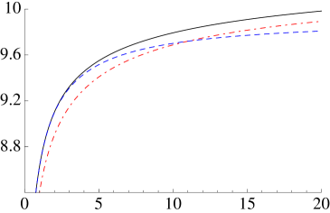
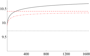
Figure 1: The mutual information for various input PDFs as a function of input average power $P$ for the parameters $Q=1.5\times 10^{-7}\,\mathrm{mW}\,\mathrm{km}^{-1}$, $\gamma=10^{-3}\,\mathrm{mW}^{-1}\mathrm{km}^{-1}$, $L=1000\,\mathrm{km}$. (a): The solid black line, blue dashed line, red dashed dotted line correspond to the optimal PDF $P_{X}^{opt}[X]$, Gaussian PDF $P_{X}^{(2)}[X]$, and half-Gaussian PDF $P_{X}^{(1)}[X]$, respectively. (b): The solid black line corresponds to $I_{P_{X}^{opt}[X]}$, see Eq. (51); the red dashed dotted line corresponds to the mutual information for the half-Gaussian distribution $I_{P_{X}^{(1)}[X]}$, see Eq. (57) for $\beta=1$; the red dashed horizontal line corresponds to our limit (59) at $\tilde{\gamma}\gg 1$ for the half-Gaussian distribution; the black dotted horizontal line corresponds to the result [14], see Eq. (10).

There is no simple analytical form for $N_{0}(P)$ and $\lambda_{0}(P)$ therefore to plot Fig. 1 and Fig 2 (see below) we calculated $\lambda_{0}(P)$ and $N_{0}(P)$ numerically. For large and small values of the parameter $\tilde{\gamma}$ we can use the solutions in Eqs. (III) and (50), respectively. At small $\tilde{\gamma}=\gamma LP/\sqrt{3}$ we obtain

$$\!\!\!I_{P_{X}^{opt}[X]}=\log\left(1+\mathrm{SNR}\right)-\tilde{\gamma}^{2}+{\cal O}(\tilde{\gamma}^{3})+{\cal O}\left(\frac{1}{{\mathrm{SNR}}}\right),$$ (53)

which is simply the Shannon capacity, $\log\left(1+\mathrm{SNR}\right)$, of the linear AWGN channel (1) with the first nonlinear correction. In Eq. (53) the unity in the logarithm is beyond the accuracy of our calculation but we keep it to bring to notice that the derived expressions (III) and (53) have the correct limit when the parameter $\gamma$ tends to zero (in contrast to the Eq. (35) in Ref. [14]). In Eq. (53) we omit the accuracy ${\cal O}\left(\gamma^{2}L^{3}QP\right)$ since the parameter $\gamma^{2}L^{3}QP$ is of order of $\tilde{\gamma}^{2}/\mathrm{SNR}$. In the second power sub-interval $(\gamma L)^{-1}\ll P\ll\left(QL^{3}\gamma^{2}\right)^{-1}$, using Eq. (III) one can see that the mutual information increases very slowly (loglog) with $P$

$$I_{P_{X}^{opt}[X]}=-\log\left({QL^{2}\gamma}\right)-1+\frac{\log 3}{2}+\log\log\left(\frac{C\gamma LP}{\sqrt{3}}\right)+$$

$$\frac{1}{\log\left({C\gamma LP}/{\sqrt{3}}\right)}\left[\log\log\left(\frac{C\gamma LP}{\sqrt{3}}\right)+1-\frac{\log\log\left({C\gamma LP}/{\sqrt{3}}\right)}{\log\left({C\gamma LP}/{\sqrt{3}}\right)}\right]+$$

$${\cal O}\left(1/\log^{2}(\gamma LP)\right)+{\cal O}\left(1/\mathrm{SNR}\right)+{\cal O}\left(\gamma^{2}L^{3}QP\right),$$ (54)

as opposed to the constant behavior of the mutual information for Gaussian-like distributions of an input signal, see formulae (58) and (59) below.

In the remainder of this Section we perform an analysis of the mutual information for the distribution $P_{X}^{(\beta)}[X]$, see Eq. (33), generalizing the half-Gaussian distribution (8) (see, for example Ref. [14]) and the Gaussian input PDF (34). In the leading order in $1/\mathrm{SNR}$ from (39) we obtain

$$\!\!\!\!\!\!\!\!\!\!H_{\beta}[Y]=\log\left(P\frac{2\pi}{\beta}\Gamma\left(\frac{\beta}{2}\right)\right)+\frac{\beta}{2}+\frac{2-\beta}{2}\psi\Big{(}\frac{\beta}{2}\Big{)},$$ (55)

where $\psi(z)$ is the digamma function $\psi(z)=\Gamma^{\prime}(z)/\Gamma(z)$, where $\psi(1)=-\gamma_{E}$ and $\psi(1/2)=-\gamma_{E}-2\log(2)$. The substitution of Eq. (33) into Eq. (III) gives

$$\!\!\!\!\!\!H_{\beta}[Y|X]=\log\Big{(}\pi eQL\Big{)}+$$

$$\frac{1}{2\Gamma\left(\frac{\beta}{2}\right)}\int^{\infty}_{0}d\tau e^{-\tau}\tau^{\beta/2-1}\log\left(1+\frac{4\tilde{\gamma}^{2}}{\beta^{2}}\tau^{2}\right)$$ (56)

with at least ${{\cal O}(1/{\mathrm{SNR}})}$ accuracy. The integral in Eq. (IV) can be calculated analytically using Ref. [21], however, the result of the integration is cumbersome, hence we do not present it here. One can easily obtain the mutual information $I_{P_{X}^{(\beta)}[X]}$ by subtracting Eq. (IV) from Eq. (55):

$$I_{P_{X}^{(\beta)}}[X] = \log\mathrm{SNR}+\log\left(\frac{2\Gamma\left(\beta/2\right)}{\beta}\right)-$$ (57)

$$\frac{1}{2\Gamma\left(\frac{\beta}{2}\right)}\int^{\infty}_{0}d\tau e^{-\tau}\tau^{\beta/2-1}\log\left(1+\frac{4\tilde{\gamma}^{2}}{\beta^{2}}\tau^{2}\right)+$$

$$\frac{\beta-2}{2}\left(1-\psi\left(\frac{\beta}{2}\right)\right)+{{\cal O}\left(\frac{1}{{\mathrm{SNR}}}\right)+{\cal O}\left(\gamma^{2}L^{3}QP\right)}.$$

The mutual information is depicted in Fig. 1(a) for the Gaussian distribution by the blue dashed line, and for the half-Gaussian by the red dashed dotted line. One can see that at small $P$ the mutual information for the Gaussian distribution is greater than that of the half-Gaussian, whereas at $P>11\mathrm{mW}$ the mutual information is greater for the half-Gaussian distribution. Note that $I_{P_{X}^{opt}[X]}$ is greater than $I_{P_{X}^{(\beta)}[X]}$ for all values of $P$, as it should be. At $\tilde{\gamma}\gg 1$ the mutual information $I_{P_{X}^{(\beta)}[X]}$ takes the form

$$I_{P_{X}^{(\beta)}[X]}\!\! = \!\!-\log\left(QL^{2}\gamma\right)-\frac{2-\beta}{2}+\frac{\log 3}{2}-\frac{\beta}{2}\psi\left(\frac{\beta}{2}\right)+$$ (58)

$$\log\left(\Gamma\left(\beta/2\right)\right)+{{\cal O}\left(\frac{1}{{\mathrm{SNR}}}\right)+{\cal O}\left(\gamma^{2}L^{3}QP\right)}.$$

One can see that at large $\mathrm{SNR}$ $I_{P_{X}^{(\beta)}[X]}$ goes to a constant in the interval of power $P$ considered, and this constant depends on the noise power $QL$. We remind that $I_{P_{X}^{opt}[X]}$ increases as $\log\log P$ in the region under consideration. The mutual information for the half-Gaussian distribution (8) in the regime $\tilde{\gamma}\gg 1$ can be obtained as a particular case of (58) for $\beta=1$:

$$I_{P_{X}^{(1)}[X]} = -\log\left({QL^{2}\gamma}\right)+\log 2+$$ (59)

$$\frac{\log 3\pi-1+\gamma_{E}}{2}+{{\cal O}\left(\frac{1}{{\mathrm{SNR}}}\right)+{\cal O}\left(\gamma^{2}L^{3}QP\right)}.$$

Comparing our expression (59) with the result (40) of Ref. [14] we have an extra term $+\log 2$ due to our more accurate calculation of $H[Y|X]$. Our result (59) and the result of Ref. [14], see Eq. (10), are presented in Fig. 1(b). In Fig. 1(b) one can see that the mutual information (51) for the optimal distribution exceeds the limit (59) at $P\sim 190$mW. At this power the difference between the limit (59) and $I_{P_{X}^{(1)}[X]}$ evaluated on the base of Eq. (57) with $\beta=1$ is of order of $1.5\%$ and getting smaller at higher $P$.

Since we have now found $P_{X}^{opt}[X]$ in the power region (23), we can calculate an approximation for the capacity of the considered per-sample nonlinear channel. By definition it coincides with the mutual information expression (51):

$$C=I_{P_{X}^{opt}[X]}.$$ (60)

Let us emphasize that this result for the capacity has accuracy ${\cal O}\left(1/{\mathrm{SNR}}\right)+{\cal O}\left(\gamma^{2}L^{3}QP\right)$, see Eq. (51). The comparison of the approximation (60) with the Shannon capacity of the linear AWGN channel is presented in Fig. 2.

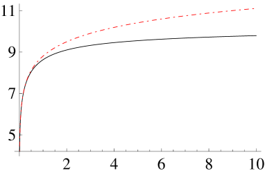
Figure 2: Shannon capacity and the capacity of the nonlinear channel $I_{P_{X}^{opt}[X]}$ for the parameters $Q=1.5\times 10^{-7}\,\mathrm{mW}\,\mathrm{km}^{-1}$, $\gamma=10^{-3}\,\mathrm{mW}^{-1}\mathrm{km}^{-1}$, $L=1000\,\mathrm{km}$. The black solid line corresponds to $I_{P_{X}^{opt}[X]}$, see Eq. (51), the red dashed-dotted line corresponds to the Shannon limit $\log[1+\mathrm{SNR}]$.

One can see that the Shannon capacity of the linear AWGN channel is always greater than the approximation (60) for the nondispersive nonlinear fiber channel for the considered region of $P$.

V Conclusion

We have developed a new approach to the calculation of the conditional PDF via the path-integral representation (14) at large $\mathrm{SNR}$ for the intermediate power region (23). This may be an especially useful technique for complex nonlinear channels in which the calculation of the conditional PDF is technically challenging. Applying our method to the per-sample nondispersive nonlinear fiber channel, we derived compact analytical expressions for the conditional PDF, conditional entropy and the entropy of the output signal for different input signal PDFs $P_{X}[X]$. Moreover, we solved the variational problem on $P_{X}[X]$ maximizing the mutual information in the leading order in $1/\mathrm{SNR}$ in the power region (23). That allows us to find the optimal input signal distribution (45) and the approximation for the channel capacity (51) up to ${1/{\mathrm{SNR}}}$ and $\gamma^{2}L^{3}QP$ corrections in the power interval $QL\ll P\ll(\gamma^{2}QL^{3})^{-1}$, which is extremely wide for realistic parameters, see (52). The found distribution $P_{X}^{opt}[X]$ is different from the half-Gaussian one, and at the zero nonlinearity $P_{X}^{opt}[X]$ approaches the Gaussian distribution. We demonstrated that the approximation found for the capacity of the channel considered here (60) is always greater than the mutual information calculated for Gaussian and half-Gaussian distributions, and lower than the Shannon capacity of the linear AWGN channel.

Acknowledgments The calculations of the next-to-leading order corrections in $1/\mathrm{SNR}$ have been performed with support of the Russian Science Foundation (RSF) (grant No. 16-11-10133). Part of the work (Section III) was supported by the Russian Scientific Foundation (RFBR), Grant No. 16-31-60031/15. A. V. Reznichenko thanks the President program for support. The work of S. K. Turitsyn was supported by the grant of the Ministry of Education and Science of the Russian Federation (agreement No. 14.B25.31.0003) and the EPSRC project UNLOC.

-A The classical solution $\Psi_{cl}$ and the action $S[\Psi_{cl}]$.

In Ref. [17] we have shown that in the case $\mathrm{SNR}={P}/{QL}\gg 1$ the conditional probability can be written in the form:

$$P[Y|X]=\exp\left\{-\frac{S[\Psi_{cl}(z)]}{Q}\right\}\!\!\int\limits_{{\psi}(0)=0}^{{\psi}(L)=0}\!\!\!\!\!{\cal D}{\psi}\,\exp\left\{-\dfrac{S[\Psi_{cl}(z)+{\psi}(z)]-S[\Psi_{cl}(z)]}{Q}\right\}\,,$$ (61)

where for the nondispersive model the effective action reads

$$S[\psi]=\int\limits_{0}^{L}dz\Big{|}\partial_{z}\psi-i\gamma|\psi|^{2}\psi\Big{|}^{2}.$$ (62)

The action (62) is associated with the l.h.s. of the nonlinear Shrödinger equation

$$\partial_{z}\psi(z)-i\gamma|\psi(z)|^{2}\psi(z)=\eta(z),$$ (63)

where the noise $\eta(z)$ has the Gaussian nature:

$$\langle\eta(z)\rangle_{\eta}=0\,,\qquad\langle\eta(z)\bar{\eta}(z^{\prime})\rangle_{\eta}=Q\delta(z-z^{\prime})\,.$$ (64)

The measure ${\cal D}{\psi}$ in Eq. (61) is defined as

$${\cal D}{\psi}=\lim_{\Delta\rightarrow 0}\Big{(}\frac{1}{\Delta\pi Q}\Big{)}^{N}\prod^{N-1}_{i=1}dRe{\psi}_{i}\,dIm{\psi}_{i},$$ (65)

here ${\psi}_{i}={\psi}(z_{i})$ and $\Delta=\frac{L}{N}$ is the grid space.

Now we consider the difference of actions in the exponent of the path-integral in Eq. (61).

$${S[\Psi_{cl}(z)+{\psi}(z)]-S[\Psi_{cl}(z)]}=$$

$$\int^{L}_{0}dz\Big{\{}\left|\partial_{z}{\psi}-i\gamma(2{\psi}|\Psi_{cl}|^{2}+\bar{\psi}\Psi^{2}_{cl})\right|^{2}+2\gamma Im\left[\left(\partial_{z}\bar{\Psi}_{cl}+i\gamma\bar{\Psi}_{cl}|{\Psi}_{cl}|^{2}\right)\left(2\Psi_{cl}|\psi|^{2}+\bar{\Psi}_{cl}\psi^{2}\right)\right]+$$

$$\gamma^{2}\left|2\Psi_{cl}|\psi|^{2}+\bar{\Psi}_{cl}\psi^{2}+\psi|\psi|^{2}\right|^{2}+2\gamma Im\left[\left(\partial_{z}\bar{\psi}+i\gamma(2\bar{\psi}|\Psi_{cl}|^{2}+{\psi}\bar{\Psi}^{2}_{cl})\right)\left(2\Psi_{cl}|\psi|^{2}+\bar{\Psi}_{cl}\psi^{2}+\psi|\psi|^{2}\right)\right]+$$

$$2\gamma Im\left[\left(\partial_{z}\bar{\Psi}_{cl}+i\gamma\bar{\Psi}_{cl}|{\Psi}_{cl}|^{2}\right)\psi|\psi|^{2}\right]\Big{\}}.$$ (66)

In Eq.  (61) the function $\Psi_{cl}(z)$ is the solution of the equation $\delta S[\Psi_{cl}]=0$ (Euler-Lagrange equation) which has the form

$$\frac{d^{2}\Psi_{cl}}{dz^{2}}-4i\gamma\left|\Psi_{cl}\right|^{2}\frac{d\Psi_{cl}}{dz}-3\gamma^{2}\left|\Psi_{cl}\right|^{4}\Psi_{cl}=0,$$ (67)

with boundary conditions $\Psi_{cl}(0)=X=|X|\exp[{i\phi^{(X)}}]$, $\Psi_{cl}(L)=Y=|Y|\exp[{i\phi^{(Y)}}]$. It is easy to find the solution of Eq.  (67) in the polar coordinate system: $\Psi_{cl}(z)=\rho(\zeta)e^{i\theta(\zeta)}$, $\zeta=z/L$. The solution depends on four real integration constants. We denote them as $E$, $\tilde{\mu}$, $\zeta_{0}$ and $\theta_{0}$. There are two different regimes of the solution: in the trigonometric regime one has $E=\frac{k^{2}}{2}\geq 0$, and in the hyperbolic regime $E=-\frac{k^{2}}{2}\leq 0$. For both cases instead of $E$ we introduce the non-negative parameter $k=\sqrt{2|E|}$.

• In the trigonometric case ($E=\frac{k^{2}}{2}\geq 0$) we have the solution for $\tilde{\mu}\geq k\geq 0$:

  $$\begin{split}&\rho^{2}(\zeta)=\frac{1}{2L\gamma}\Big{(}\tilde{\mu}+\sqrt{\tilde{\mu}^{2}-k^{2}}\cos[2k(\zeta-\zeta_{0})]\Big{)}\,,\\ &\theta(\zeta)=\frac{\tilde{\mu}}{2}(\zeta-\zeta_{0})+\sqrt{\tilde{\mu}^{2}-k^{2}}\,\frac{\sin[2k(\zeta-\zeta_{0})]}{4k}+\arctan\left[(\tilde{\mu}-\sqrt{\tilde{\mu}^{2}-k^{2}})\frac{\tan[k(\zeta-\zeta_{0})]}{k}\right]+\theta_{0}.\end{split}$$ (68)

  Here the integration constants $\tilde{\mu}$, $k$ and $\zeta_{0}$ must be found from the boundary conditions:

  $$|X|^{2}=\rho^{2}(0)=\frac{1}{2L\gamma}\Big{(}\tilde{\mu}+\sqrt{\tilde{\mu}^{2}-k^{2}}\cos[2k\zeta_{0}]\Big{)},$$ (69)

  $$|Y|^{2}=\rho^{2}(1)=\frac{1}{2L\gamma}\Big{(}\tilde{\mu}+\sqrt{\tilde{\mu}^{2}-k^{2}}\cos[2k(1-\zeta_{0})]\Big{)},$$ (70)

  $$\phi^{(X)}=\theta(0)=-\frac{\tilde{\mu}}{2}\zeta_{0}-\sqrt{\tilde{\mu}^{2}-k^{2}}\,\frac{\sin[2k\zeta_{0}]}{4k}-\arctan\left[(\tilde{\mu}-\sqrt{\tilde{\mu}^{2}-k^{2}})\frac{\tan[k\zeta_{0}]}{k}\right]+\theta_{0},$$ (71)

  $$\phi^{(Y)}=\theta(1)=\frac{\tilde{\mu}}{2}(1-\zeta_{0})+\sqrt{\tilde{\mu}^{2}-k^{2}}\,\frac{\sin[2k(1-\zeta_{0})]}{4k}+\arctan\left[(\tilde{\mu}-\sqrt{\tilde{\mu}^{2}-k^{2}})\frac{\tan[k(1-\zeta_{0})]}{k}\right]+\theta_{0}.$$ (72)

  Then one can find the action

  $$S[\Psi_{cl}(z;E=\frac{k^{2}}{2},\tilde{\mu},\zeta_{0},\theta_{0})]=\frac{k^{2}}{2\gamma L}\left({\tilde{\mu}}-\sqrt{\tilde{\mu}^{2}-k^{2}}\,\frac{\sin[2k(1-\zeta_{0})]+\sin[2k\zeta_{0}]}{2k}\right).$$ (73)

• In the hyperbolic case ($E=-\frac{k^{2}}{2}\leq 0$) we have the solution for $k\geq 0$ and arbitrary $\tilde{\mu}$ in the following form

  $$\begin{split}&\rho^{2}(\zeta)=\frac{1}{2L\gamma}\Big{(}-\tilde{\mu}+\sqrt{\tilde{\mu}^{2}+k^{2}}\cosh[2k(\zeta-\zeta_{0})]\Big{)}\,,\\ &\theta(\zeta)=-\frac{\tilde{\mu}}{2}(\zeta-\zeta_{0})+\sqrt{\tilde{\mu}^{2}+k^{2}}\,\frac{\sinh[2k(\zeta-\zeta_{0})]}{4k}-\arctan\left[(\tilde{\mu}+\sqrt{\tilde{\mu}^{2}+k^{2}})\frac{\tanh[k(\zeta-\zeta_{0})]}{k}\right]+\theta_{0},\end{split}$$ (74)

  where $\tilde{\mu}$, $k$, $\zeta_{0}$, and $\theta_{0}$ are derived from the same procedure as in the trigonometric regime. The action reads

  $$S[\Psi_{cl}(z;E=-\frac{k^{2}}{2},\tilde{\mu},\zeta_{0},\theta_{0})]=\frac{k^{2}}{2\gamma L}\left({\tilde{\mu}}+\sqrt{\tilde{\mu}^{2}+k^{2}}\,\frac{\sinh[2k(1-\zeta_{0})]+\sinh[2k\zeta_{0}]}{2k}\right).$$ (75)

Note, there are two solutions of Eq. (67) with constant $\rho(z)=\rho(0)\equiv\rho$ obeying only the input boundary condition $\Psi_{0}(0)=X$. The first one reads

$$\Psi_{0}(z)=\rho\exp\left\{i\mu\frac{z}{L}+i\phi^{(X)}\right\},$$ (76)

where $\mu=\gamma L\rho^{2}=\gamma L|X|^{2}$. This function corresponds to the solution representation (68) with $k=0$ and $\tilde{\mu}=\mu$ or to the solution representation (74) with $k=0$ and $\tilde{\mu}=-\mu$. The function $\Psi_{0}(z)$ is the solution of the Eq.  (63) with zero noise and with the input boundary condition. Furthermore, $\Psi_{0}(z)$ delivers the absolute minimum of the action (62): $S[\Psi_{0}(z)]=0$. The second solution of Eq. (67) with constant $\rho(z)$ is the trigonometric regime (68) case with $\tilde{\mu}=k=2\mu$:

$$\Psi_{\rho=const}(z)=\rho\exp\left\{3i\,\mu\frac{z}{L}+i\phi^{(X)}\right\},\qquad\mu=\gamma L\rho^{2}=\gamma L|X|^{2}.$$ (77)

To find the solution of Eq. (67) one should express the integration constant through the boundary conditions. Instead, we exploit the fact that the noise power $QL$ is much less than the input signal power $P=|X|^{2}\equiv\rho^{2}$. In other words, we will find a solution of Eq. (67) that is close to $\Psi_{0}(z)$: it is the solution of Eq. (63) with zero noise which provides the absolute minimum of the action $S[\Psi_{0}(z)]=0$. In that fashion we perform the substitution in Eq. (67):

$$\Psi_{cl}(z)=(\rho+\varkappa(z))\exp\left\{i\mu\frac{z}{L}+i\phi^{(X)}\right\},$$ (78)

where the function $\varkappa(z)$ is assumed to be small: $\varkappa(z)\ll\rho$ for all configurations of $\Psi_{cl}(z)$ providing $S[\Psi_{cl}(z)]/Q={\cal O}(1)$ when $QL$ tends to zero. We have the following equation on $\varkappa(z)$ resulting from the Eq. (67):

$$\frac{d^{2}\varkappa}{dz^{2}}-2i\frac{\mu}{L}\frac{d\varkappa}{dz}-4\frac{\mu^{2}}{L^{2}}Re[\varkappa]=4i\frac{\mu}{L\rho}\left(\varkappa+\bar{\varkappa}\right)\frac{d\,\varkappa}{dz}+\frac{\mu^{2}}{L^{2}\rho}\left[5\varkappa^{2}+10|\varkappa|^{2}+3\bar{\varkappa}^{2}\right]+$$

$$\frac{|\varkappa|^{2}\mu}{L^{2}\rho^{2}}\left[4iL\frac{d\varkappa}{dz}+9{\mu}\bar{\varkappa}+14{\mu}{\varkappa}\right]+\frac{3\mu^{2}}{L^{2}\rho^{2}}\varkappa^{3}+\frac{3\mu^{2}}{L^{2}\rho^{3}}|\varkappa|^{2}\left[3|\varkappa|^{2}+2\varkappa^{2}\right]+\frac{3\mu^{2}}{L^{2}\rho^{4}}|\varkappa|^{4}\varkappa.$$ (79)

We present $\varkappa(z)$ as a perturbation theory decomposition in powers of $1/\sqrt{\mathrm{SNR}}$: $\varkappa(z)=\varkappa_{1}(z)+\varkappa_{2}(z)+\ldots$, where $\varkappa_{1}(z)$ is of $1/\sqrt{\mathrm{SNR}}$ order and provides the leading order contribution, $\varkappa_{2}(z)$ is of $1/{\mathrm{SNR}}$ order, and so on.

• The linearized equation for the function $\varkappa_{1}(z)=x_{1}(z)+iy_{1}(z)$ can be obtained from Eq. (-A) by omitting the r.h.s. of this equation:

  $$\frac{d^{2}\varkappa_{1}}{dz^{2}}-2i\frac{\mu}{L}\frac{d\varkappa_{1}}{dz}-4\frac{\mu^{2}}{L^{2}}Re[\varkappa_{1}]=0.$$ (80)

  The boundary conditions $\Psi_{cl}(0)=X$ and $\Psi_{cl}(1)=Y\equiv\rho^{\prime}e^{i\phi^{(Y)}}$ lead to

  $$\varkappa_{1}(0)=0,$$

  $$\varkappa_{1}(L)=x_{0}+iy_{0}=\rho^{\prime}e^{i(\phi^{(Y)}-\phi^{(X)}-\mu)}-\rho.$$ (81)

  The solution $\varkappa_{1}(z)=x_{1}(z)+iy_{1}(z)$ of the linearized boundary problem (80), (• ‣ -A) is polynomial

  $$x_{1}(z)=\Big{(}-\mu a_{1}(X,Y)\frac{z}{L}+a_{2}(X,Y)\Big{)}\frac{z}{L},$$

  $$y_{1}(z)=\Big{(}-\frac{2}{3}\mu^{2}a_{1}(X,Y)\frac{z^{2}}{L^{2}}+\mu\,a_{2}(X,Y)\frac{z}{L}+a_{1}(X,Y)\Big{)}\frac{z}{L},$$ (82)

  where coefficients $a_{1}(X,Y)$ and $a_{2}(X,Y)$ can be found from the boundary conditions (• ‣ -A) and have the form:

  $$a_{1}(X,Y)=\frac{-\mu x_{0}+y_{0}}{1+\mu^{2}/3},\qquad a_{2}(X,Y)=\frac{(1-2\mu^{2}/3)x_{0}+\mu y_{0}}{1+\mu^{2}/3},$$ (83)

  with $x_{0}=x_{0}(X,Y)$ and $y_{0}=y_{0}(X,Y)$ being determined from Eq. (• ‣ -A). In the leading order the action reads

  $$\frac{1}{Q}S\left[\Psi_{0}(z)+\varkappa_{1}(z)e^{i\mu\frac{z}{L}+i\phi^{(X)}}\right]=\frac{1}{Q}\int^{L}_{0}dz\left[\left|\partial_{z}\varkappa_{1}-2i\frac{\mu}{L}Re[\varkappa_{1}]\right|^{2}+{\cal O}\left(\frac{\varkappa_{1}^{3}}{\rho^{3}}\right)\right]=$$

  $$=\frac{(1+4\mu^{2}/3)a^{2}_{1}-2\mu a_{1}a_{2}+a^{2}_{2}}{QL}+{\cal O}\left(\frac{1}{\sqrt{\mathrm{SNR}}}\right)=\frac{(1+4\mu^{2}/3)x^{2}_{0}-2\mu x_{0}y_{0}+y^{2}_{0}}{QL(1+\mu^{2}/3)}+{\cal O}\left(\frac{1}{\sqrt{\mathrm{SNR}}}\right).$$ (84)

• Let us proceed to the next-to-leading order correction to $P[Y|X]$. We should calculate the next approximation $\varkappa_{2}(z)$ to the solution (78). Taking into account Eq. (80) we present the equation for $\varkappa_{2}(z)$ in the form

  $$\frac{d^{2}\varkappa_{2}}{dz^{2}}-2i\frac{\mu}{L}\frac{d\varkappa_{2}}{dz}-4\frac{\mu^{2}}{L^{2}}Re[\varkappa_{2}]=4i\frac{\mu}{L\rho}\left(\varkappa_{1}+\bar{\varkappa}_{1}\right)\frac{d\,\varkappa_{1}}{dz}+\frac{\mu^{2}}{L^{2}\rho}\left[5\varkappa_{1}^{2}+10|\varkappa_{1}|^{2}+3\bar{\varkappa_{1}}^{2}\right],$$ (85)

  where the boundary conditions for $\varkappa_{2}(z)$ read $\varkappa_{2}(0)=\varkappa_{2}(L)=0$. The solution $\varkappa_{2}(z)=x_{2}(z)+iy_{2}(z)$ of Eq. (85) is polynomial in $z$ and quadratic in $x_{0}$ and $y_{0}$:

  $$\begin{split}x_{2}(z)=&-\frac{\mu/\rho}{270(1+\mu^{2}/3)^{3}}\Big{(}1-\frac{z}{L}\Big{)}\frac{z}{L}\times\\ &\Big{\{}\mu\left(2\mu^{4}-15\mu^{2}+585\right)x^{2}_{0}+2\left(13\mu^{2}\left(\mu^{2}+15\right)-180\right)x_{0}y_{0}+\mu\left(2\mu^{2}+15\right)\left(5\mu^{2}-9\right)y^{2}_{0}-\\ &5\left(\mu^{2}+3\right)\frac{z}{L}\left(\mu\left(\mu^{2}-15\right)x^{2}_{0}-4\left(\mu^{2}-6\right)x_{0}y_{0}+\mu\left(\mu^{2}+9\right){y^{2}_{0}}\right)+\\ &5\mu\left(\mu^{2}+3\right)\frac{z^{2}}{L^{2}}\left(3\left(5\mu^{2}-3\right)x^{2}_{0}-36\mu x_{0}y_{0}-\left(\mu^{2}-15\right)y^{2}_{0}\right)+\\ &20\mu^{2}\left(\mu^{2}+3\right)\frac{z^{3}}{L^{3}}(y_{0}-\mu x_{0})\left(2\mu y_{0}-\left(\mu^{2}-3\right)x_{0}\right)-\\ &20\mu^{3}\left(\mu^{2}+3\right)\frac{z^{4}}{L^{4}}(y_{0}-\mu x_{0})^{2}\Big{\}}.\end{split}$$ (86)

  $$\begin{split}y_{2}(z)=&-\frac{\mu/\rho}{270(1+\mu^{2}/3)^{3}}\Big{(}1-\frac{z}{L}\Big{)}\frac{z}{L}\times\\ &\Big{\{}\left(7\mu^{4}-75\mu^{2}+360\right)x^{2}_{0}+6\mu\left(\mu^{2}+75\right)x_{0}y_{0}+3\mu^{2}\left(5\mu^{2}+39\right)y^{2}_{0}+\\ &2\frac{z}{L}\left(\left(\mu^{6}-4\mu^{4}+255\mu^{2}+180\right)x^{2}_{0}+\mu\left(\mu^{2}+15\right)\left(13\mu^{2}+3\right)x_{0}y_{0}+\mu^{2}\left(5\mu^{4}+36\mu^{2}-9\right)y^{2}_{0}\right)-\\ &14\mu\left(\mu^{2}+3\right)\frac{z^{2}}{L^{2}}(y_{0}-\mu x_{0})\left(\left(15-4\mu^{2}\right)x_{0}+9\mu y_{0}\right)+\\ &84\mu^{2}\left(\mu^{2}+3\right)\frac{z^{3}}{L^{3}}(y_{0}-\mu x_{0})^{2}\Big{\}}.\end{split}$$ (87)

  In the leading, see Eq. (• ‣ -A), and next-to-leading order in $1/\sqrt{\mathrm{SNR}}$ the action reads

  $$\begin{split}&\frac{1}{Q}S[\Psi_{cl}(z)]=\frac{(1+4\mu^{2}/3)x^{2}_{0}-2\mu x_{0}y_{0}+y^{2}_{0}}{QL(1+\mu^{2}/3)}+\frac{\mu/\rho}{135QL\left(1+\mu^{2}/3\right)^{3}}\Big{\{}\mu\left(4\mu^{4}+15\mu^{2}+225\right)x^{3}_{0}+\\ &{\left(23\mu^{4}+255\mu^{2}-90\right)x^{2}_{0}y_{0}+\mu\left(20\mu^{4}+117\mu^{2}-45\right)x_{0}y^{2}_{0}-3\left(5\mu^{4}+33\mu^{2}+30\right)y^{3}_{0}}\Big{\}}+{\cal O}\left(\frac{1}{{\mathrm{SNR}}}\right).\end{split}$$ (88)

-B The path-integral calculation.

To calculate the conditional probability density $P[Y|X]$ in Eq. (61) one should find the pre-exponent path-integral, referred to as the quantum corrections near the classical solution $\Psi_{cl}(z)$, in the leading and next-to-leading order in $1/\sqrt{\mathrm{SNR}}$:

$$I_{QC}[\Psi_{cl}(z)]=\int\limits_{\tilde{\psi}(0)=0}^{{\psi}(L)=0}\!\!\!\!\!{\cal D}{\psi}\,\exp\left\{-\dfrac{S[\Psi_{cl}(z)+{\psi}(z)]-S[\Psi_{cl}(z)]}{Q}\right\}.$$ (89)

In what follows we are interested in the leading and next-to-leading order corrections for the path-integral (61). That is why we retain only quadratic in $\psi$ terms in Eq. (-A). All these terms are placed in the second line of Eq. (-A). As it will be demonstrated below an extra power of $\psi$ results in an extra power of $\sqrt{QL}$. In the leading and next-to-leading order calculation of the path-integral we should take into account the first correction ($\varkappa_{1}(z)\propto\sqrt{QL}$) to the solution $\Psi_{cl}(z)$, see Eqs. (78) and (• ‣ -A). Now we put (78) with $\varkappa_{1}(z)$ and $\psi(z)$ in the form $\psi(z)=u(z)\exp\left\{i\mu\frac{z}{L}+i\phi^{(X)}\right\}$ into the first line of Eq. (-A). In our approximation we obtain

$${S[\Psi_{cl}(z)+{\psi}(z)]-S[\Psi_{cl}(z)]}=\int^{L}_{0}dz\Big{\{}\left|\partial_{z}u-i\frac{\mu}{L}(u+\bar{u})\right|^{2}+$$

$$2\frac{\mu}{L\rho}Im\left[2\Big{(}\partial_{z}\bar{u}+i\frac{\mu}{L}(u+\bar{u})\Big{)}\Big{(}u(\varkappa_{1}+\bar{\varkappa}_{1})+\bar{u}\varkappa_{1}\Big{)}+\Big{(}\partial_{z}\bar{\varkappa}_{1}+i\frac{\mu}{L}(\varkappa_{1}+\bar{\varkappa}_{1})\Big{)}\Big{(}2|u|^{2}+u^{2}\Big{)}\right]+$$

$${\cal O}\left(\frac{\gamma}{L}u^{2}\varkappa^{2}_{1}\right)+{\cal O}\left(\frac{\gamma}{L}\rho u^{2}\varkappa_{2}\right)+{\cal O}\left(\gamma^{2}\rho^{2}u^{4}\right)\Big{\}}.$$ (90)

We substitute this difference in the exponent in Eq. (89). Then we expand the exponent at small $Q$ and obtain:

$$\exp\left\{-\dfrac{S[\Psi_{cl}(z)+{\psi}(z)]-S[\Psi_{cl}(z)]}{Q}\right\}=\exp\Big{\{}-\frac{1}{Q}\int^{L}_{0}dz\Big{|}\partial_{z}u-i\frac{\mu}{L}(u+\bar{u})\Big{|}^{2}\Big{\}}\Big{\{}1-$$

$$\frac{2\mu}{QL\rho}Im\int^{L}_{0}dz\left[2\Big{(}\partial_{z}\bar{u}+i\frac{\mu}{L}(u+\bar{u})\Big{)}\Big{(}u(\varkappa_{1}+\bar{\varkappa}_{1})+\bar{u}\varkappa_{1}\Big{)}+\Big{(}\partial_{z}\bar{\varkappa}_{1}+i\frac{\mu}{L}(\varkappa_{1}+\bar{\varkappa}_{1})\Big{)}\Big{(}2|u|^{2}+u^{2}\Big{)}\right]+$$

$${\cal O}\left(\frac{QL}{\rho^{2}}\right)+{\cal O}\left(\gamma^{2}QL^{3}\rho^{2}\right)\Big{\}}.$$ (91)

Here we imply that any extra power of $u$ or $\varkappa$ is suppressed by the multiplicative parameter $\sqrt{QL}$, because at small $Q$ the main contribution to the path-integral comes from $u\sim\sqrt{QL}$. We substitute this expansion (-B) into the path-integral (89) and change the variable from ${\psi}(z)$ to $u(z)$ and arrive at

$$I_{QC}[\Psi_{0}(z)]=\int\limits_{u(0)=0}^{u(L)=0}\!\!\!\!\!{\cal D}u\,\exp\Big{\{}-\frac{1}{Q}\int^{L}_{0}dz\Big{|}\partial_{z}u-i\frac{\mu}{L}(u+\bar{u})\Big{|}^{2}\Big{\}}\Big{[}1-$$

$$\frac{2\mu}{QL\rho}Im\int^{L}_{0}dz\left[2\Big{(}\partial_{z}\bar{u}+i\frac{\mu}{L}(u+\bar{u})\Big{)}\Big{(}u(\varkappa_{1}+\bar{\varkappa}_{1})+\bar{u}\varkappa_{1}\Big{)}+\Big{(}\partial_{z}\bar{\varkappa}_{1}+i\frac{\mu}{L}(\varkappa_{1}+\bar{\varkappa}_{1})\Big{)}\Big{(}2|u|^{2}+u^{2}\Big{)}\right]+$$

$${\cal O}\left(\frac{QL}{\rho^{2}}\right)+{\cal O}\left(\gamma^{2}QL^{3}\rho^{2}\right)\Big{]}.$$ (92)

To calculate the leading and next-to-leading order contributions to $I_{QC}[\Psi_{0}(z)]$ in $1/\mathrm{SNR}$ we should take the first and the second terms in the square brackets in Eq. (-B), respectively. We start our consideration from the leading order. In this case we represent the path-integral $I^{(0)}_{QC}[\Psi_{0}(z)]=\int_{u(0)=0}^{u(L)=0}{\cal D}u\,\exp\Big{\{}-\frac{1}{Q}\int^{L}_{0}dz\Big{|}\partial_{z}u-i\frac{\mu}{L}(u+\bar{u})\Big{|}^{2}\Big{\}}$ in the retarded discretization scheme:

$$I^{(0)}_{QC}[\Psi_{0}(z)]=\int\limits_{u(0)=0}^{u(L)=0}\!\!\!\!\!{\cal D}u\,\exp\Big{\{}-\frac{1}{Q}\int^{L}_{0}dz\Big{|}\partial_{z}u-i\frac{\mu}{L}(u+\bar{u})\Big{|}^{2}\Big{\}}=$$

$$\lim_{N\rightarrow\infty}\left(\frac{N}{\pi QL}\right)^{N}\int^{\infty}_{-\infty}\prod^{N-1}_{i=1}du^{(1)}_{i}du^{(2)}_{i}\exp\left\{-\frac{N}{QL}\sum^{N-1}_{i=0}\Big{\{}(u^{(1)}_{i+1}-u^{(1)}_{i})^{2}+(u^{(2)}_{i+1}-u^{(2)}_{i}-2\frac{\mu}{N}u^{(1)}_{i})^{2}\Big{\}}\right\},$$ (93)

where we use the measure (65) and the notations $u(z_{j})=u^{(1)}_{j}+iu^{(2)}_{j}$, $z_{i}=\Delta\,i$, $\Delta=\frac{L}{N}$ and $u^{(1)}_{0}=u^{(1)}_{N+1}=u^{(2)}_{0}=u^{(2)}_{N+1}=0$. The sequential integration over $u^{(2)}_{N-1}$, $u^{(2)}_{N-2}$, $\ldots$, $u^{(2)}_{1}$ is trivial:

$$\int dY\exp\left\{-\frac{(A-Y)^{2}}{2\tau_{1}}-\frac{(Y-B)^{2}}{2\tau_{2}}\right\}=\left(2\pi\frac{\tau_{1}\tau_{2}}{\tau_{1}+\tau_{2}}\right)^{1/2}\exp\left\{-\frac{(A-B)^{2}}{2(\tau_{1}+\tau_{2})}\right\}.$$ (94)

It leads to the remaining integral (over $u^{(1)}_{i}$, $i=1,\ldots,N-1$) of the form

$$\lim_{N\rightarrow\infty}\left(\frac{N}{\pi QL}\right)^{N}\frac{(\pi QL/N)^{\frac{N-1}{2}}}{\sqrt{N}}\int^{\infty}_{-\infty}\prod^{N-1}_{i=1}du^{(1)}_{i}\exp\left\{-\frac{N}{QL}\sum^{N-1}_{i,j=1}u^{(1)}_{i}M_{i,j}(\alpha)u^{(1)}_{j}\right\},$$ (95)

where we denote $\alpha=\frac{4}{N}\Big{(}\frac{\mu}{N}\Big{)}^{2}$, and the $(N-1)$ by $(N-1)$ matrix $M(\alpha)$ has the following elements: $M_{i,i}=2+\alpha$, $M_{i,i\pm 1}=-1+\alpha$, $i=1,\ldots,N-1$, $M_{i,j}=\alpha$, $j\neq i,j\neq i\pm 1$. It is straightforward to calculate the determinant of $M(\alpha)$ and hence to perform the Gaussian integration over $u^{(1)}_{i}$

$$\det[M(\alpha)]=N+\alpha\frac{N^{2}(N^{2}-1)}{12},$$ (96)

$$I^{(0)}_{QC}[\Psi_{0}(z)]=\frac{1}{\pi QL\sqrt{1+\mu^{2}/3}}.$$ (97)

To calculate the next-to-leading order contribution to the path-integral (-B) we should take the second term in the square brackets in Eq. (-B). To find this correction we should calculate the integral (the correlator):

$$\langle u^{(\alpha)}(z)u^{(\beta)}(z^{\prime})\rangle\equiv\frac{1}{I^{(0)}_{QC}[\Psi_{0}(z)]}\int\limits_{u(0)=0}^{u(L)=0}\!\!\!\!\!{\cal D}u\,e^{-\frac{1}{Q}\int^{L}_{0}dz\Big{|}\partial_{z}u-i\frac{\mu}{L}(u+\bar{u})\Big{|}^{2}}u^{(\alpha)}(z)u^{(\beta)}(z^{\prime})=QL\,G^{\alpha,\,\beta}(z,z^{\prime}),$$ (98)

where we have introduced the dimensionless Green matrix $G^{\alpha,\,\beta}(z,z^{\prime})$, $\alpha,\,\beta=1,\,2$. The standard method for the Green matrix calculation is the calculation of the generating functional [18]:

$$Z[J_{1},J_{2}]=\int\limits_{u(0)=0}^{u(L)=0}\!\!\!\!\!{\cal D}u\,\exp\Big{\{}-\frac{1}{Q}\int^{L}_{0}dz\Big{|}\partial_{z}u-i\frac{\mu}{L}(u+\bar{u})\Big{|}^{2}+\int^{L}_{0}dz\left(J_{1}(z)u^{(1)}(z)+J_{2}(z)u^{(2)}(z)\right)\Big{\}},$$ (99)

then any correlator can be derived from the variation of the $Z[J_{1},J_{2}]$ over $J_{\alpha}$, for example

$$\langle u^{(\alpha)}(z)u^{(\beta)}(z^{\prime})\rangle=\frac{1}{Z[J_{1},J_{2}]}\frac{\delta Z[J_{1},J_{2}]}{\delta J_{\alpha}(z)\delta J_{\beta}(z^{\prime})}\Big{|}_{J_{1}=0,\,J_{2}=0}.$$ (100)

The calculation of the generating functional can be performed in the same way as the calculation of the normalization integral (-B): the integration over $u^{(2)}_{j}$ followed by the integration over $u^{(1)}_{j}$. The only new element in the calculation of the Gaussian integrals with the sources $J_{\alpha}$ is the inverse matrix $M(\alpha)^{-1}_{i,j}$ for $M(\alpha)_{i,j}=\alpha+2\delta_{i,j}-\delta_{i,j+1}-\delta_{i+1,j}$ defined herein above, see the text after Eq. (95). The calculation is simple (after the observation that $\det[M(\alpha)]M(\alpha)^{-1}_{i,j}$ is linear in $\alpha$), and we only set out the result

$$M(\alpha)^{-1}_{i,j}=N\left[\frac{i}{N}\left(1-\frac{j}{N}\right)\theta(i\leq j)+\frac{j}{N}\left(1-\frac{i}{N}\right)\theta(i>j)-\frac{\alpha N^{4}}{4\det[M(\alpha)]}\frac{i}{N}\left(1-\frac{i}{N}\right)\frac{j}{N}\left(1-\frac{j}{N}\right)\right],$$ (101)

where $\det[M(\alpha)]$ is given by Eq.  (96), and $\lim_{N\to\infty}\left(\alpha N^{4}/(4\det[M(\alpha)])\right)=3\mu^{2}/(3+\mu^{2})$. We present the result of the generating functional calculation in the form of a Green matrix convolution with the sources $J_{\alpha}$:

$$Z[J_{1},J_{2}]=\frac{1}{\pi QL\sqrt{1+\mu^{2}/3}}\exp\left\{\frac{QL}{2}\int^{L}_{0}dz\int^{L}_{0}dz^{\prime}J_{\alpha}(z)G^{\alpha,\,\beta}(z,z^{\prime})J_{\beta}(z^{\prime})\right\},$$ (102)

where the Green matrix is Hermitian and it has the following elements:

$$G^{1,\,1}(z,z^{\prime})=G^{1,\,1}(z^{\prime},z)=\left\{\theta(z^{\prime}-z)\frac{z}{2L}\left(1-\frac{z^{\prime}}{L}\right)-\frac{3\mu^{2}}{4(3+\mu^{2})}\left(1-\frac{z}{L}\right)\left(1-\frac{z^{\prime}}{L}\right)\frac{zz^{\prime}}{L^{2}}\right\}+\{z\leftrightarrow z^{\prime}\},$$ (103)

$$G^{1,\,2}(z,z^{\prime})=G^{2,\,1}(z^{\prime},z)=\frac{\mu}{2(3+\mu^{2})}\Bigg{\{}\theta(z-z^{\prime})\frac{z^{\prime}}{L}\left(1-\frac{z}{L}\right)\left(3\frac{z^{\prime}}{L}-3\frac{z}{L}+\frac{z^{\prime}}{L}\mu^{2}\Big{[}1+\frac{z}{L}\Big{(}2\frac{z^{\prime}}{L}-3\Big{)}\Big{]}\right)+$$ (104)

$$\theta(z^{\prime}-z)\frac{z}{L}\left(1-\frac{z^{\prime}}{L}\right)\left(3\frac{z^{\prime}}{L}-3\frac{z}{L}+\Big{(}\frac{z^{\prime}}{L}-1\Big{)}\mu^{2}\Big{[}\frac{z}{L}+2\frac{z^{\prime}}{L}\Big{(}\frac{z}{L}-1\Big{)}\Big{]}\right)\Bigg{\}},$$

$$G^{2,\,2}(z,z^{\prime})=G^{2,\,2}(z^{\prime},z)=\Bigg{\{}\frac{\theta(z-z^{\prime})}{6(3+\mu^{2})}\Big{(}1-\frac{z}{L}\Big{)}\frac{z^{\prime}}{L}\Bigg{[}9+3\mu^{2}\Big{(}1+\frac{z}{L}-2\frac{z^{2}}{L^{2}}+3\frac{zz^{\prime}}{L^{2}}-2\frac{z^{\prime 2}}{L^{2}}\Big{)}+$$

$$2\mu^{4}\frac{z^{\prime}}{L}\Big{(}\frac{z}{L}-1\Big{)}\Big{(}\frac{z^{\prime}}{L}-3\frac{z}{L}+2\frac{zz^{\prime}}{L^{2}}\Big{)}\Bigg{]}\Bigg{\}}+\{z\leftrightarrow z^{\prime}\}.$$ (105)

The second way to obtain the expression for the correlator (98) and Eqs. (103)-(-B) reflects the fact that the Gaussian integral (99) is saturated in the vicinity of the saddle-point solution of the equation of motion (i.e. the Euler-Lagrange equation for the action in question) [19]. Thus to find it we should solve the set of equations

$$\hat{K}_{\alpha,\gamma}G^{\gamma,\beta}(z,z^{\prime})=\frac{1}{L}\delta^{\beta}_{\alpha}\delta(z-z^{\prime}),$$ (106)

where the matrix differentiation operator $\hat{K}$ for the functions $u(z=0)=u(z=L)=0$ is defined as

$$-\frac{1}{Q}\int^{L}_{0}dz\Big{|}\partial_{z}u-i\frac{\mu}{L}(u+\bar{u})\Big{|}^{2}=-\frac{1}{2Q}\int^{L}_{0}dzu^{(\alpha)}(z)\hat{K}_{\alpha,\beta}u^{(\beta)}(z),$$ (107)

and it has the form

$$\hat{K}=2\begin{pmatrix}-\partial^{2}_{z}+\frac{4\mu^{2}}{L^{2}},&-2\frac{\mu}{L}\partial_{z}&\\ 2\frac{\mu}{L}\partial_{z},&-\partial^{2}_{z}&\end{pmatrix}.$$ (108)

The boundary conditions for equations (106) are as follows: $G^{\alpha,\beta}(z=0,z^{\prime})=G^{\alpha,\beta}(z=L,z^{\prime})=0$. The problem has the unambiguous solution (103)-(-B). Note that the homogeneous solution of the Eq. (106) is governed by the solutions of Eq.  (80) obtained above.

Using the correlator (98) with (103)-(-B) one can easily calculate the first correction presented in the second line of Eq.  (-B). This term is proportional to $\varkappa_{1}(z)\propto\sqrt{QL}$ hence delivering the first correction in $1/\sqrt{\mathrm{SNR}}$ to the leading term (97). The subsequent integration of the elements (103)-(-B) with the solution (• ‣ -A) for $\varkappa_{1}(z)$ is trivial, however the proper way to understand the discontinuous derivatives of the Green matrix elements (103)-(-B) at the same point $z^{\prime}=z$ is the retarded scheme adopted in our approach [17]: $\partial_{z}G^{\alpha,\beta}(z,z^{\prime})|_{z^{\prime}=z}\rightarrow\partial_{z}G^{\alpha,\beta}(z+0,z^{\prime})|_{z^{\prime}=z}$. Finally we have

$$I_{QC}[\Psi_{0}(z)]=\frac{1}{\pi QL\sqrt{1+\mu^{2}/3}}\Bigg{[}1-\frac{\mu/\rho}{15(1+\mu^{2}/3)^{2}}\left(\mu(15+\mu^{2})x_{0}-2(5-\mu^{2}/3)y_{0}\right)+$$

$${\cal O}\left(\frac{QL}{\rho^{2}}\right)+{\cal O}\left(\gamma^{2}QL^{3}\rho^{2}\right)\Bigg{]}.$$ (109)

The error estimation ${\cal O}\left({QL}/{\rho^{2}}\right)={\cal O}\left(1/\mathrm{SNR}\right)$ comes from taking into account the next term in the $\Psi_{cl}$ expansion of the complete action expression (-A). The estimation ${\cal O}\left(\gamma^{2}QL^{3}\rho^{2}\right)$ appears as the estimation of the contribution of the nonlinear biquadratic terms, see Eq. (-B), originating from the third line in the action (-A). Indeed, it is obvious from the expression (98) that any extra power of the field $u(z)$ results in an extra factor $\sqrt{QL}$. Substituting the leading order expression for $\Psi_{cl}$ in the third line of Eq. (-A) for these terms we arrive at the estimation ${\cal O}\left(\gamma^{2}QL^{3}\rho^{2}\right)$. That is why the formal parameter of the perturbation theory for the nonlinear terms is $QL\gamma^{2}L^{2}\rho^{2}$. Note the quantity $QL\gamma^{2}L^{2}\rho^{2}\equiv N\gamma^{2}L^{2}P$ is the very parameter determining the upper limit of the intermediate power region (23).

Finally, from Eq.  (88) for the exponent factor and from Eq. (-B) for the pre-exponent factor we arrive at the expression

$$\!\!\!P[Y|X]=\dfrac{\exp\left\{-\dfrac{(1+4\mu^{2}/3)x^{2}_{0}-2\mu x_{0}y_{0}+y^{2}_{0}}{QL(1+\mu^{2}/3)}\right\}}{\pi QL\sqrt{1+\mu^{2}/3}}\Bigg{(}1-\frac{\mu/\rho}{15(1+\mu^{2}/3)^{2}}\left(\mu(15+\mu^{2})x_{0}-2(5-\mu^{2}/3)y_{0}\right)-$$

$$\frac{\mu/\rho}{135QL\left(1+\mu^{2}/3\right)^{3}}\Big{\{}\mu\left(4\mu^{4}+15\mu^{2}+225\right)x^{3}_{0}+\left(23\mu^{4}+255\mu^{2}-90\right)x^{2}_{0}y_{0}+\mu\left(20\mu^{4}+117\mu^{2}-45\right)x_{0}y^{2}_{0}-$$

$$3\left(5\mu^{4}+33\mu^{2}+30\right)y^{3}_{0}\Big{\}}+{\cal O}\Big{(}\frac{QL}{\rho^{2}}\Big{)}+{\cal O}\left(\gamma^{2}QL^{3}\rho^{2}\right)\Bigg{)}.$$ (110)

Now it is easy to show, that the normalization condition

$$\int DYP[Y|X]=1$$ (111)

is fulfilled.

-C Calculation of $P_{out}[Y]$.

Let us consider the integral $P_{out}[Y]=\int{\cal D}XP_{X}[X]P[Y|X]$. In our case the measure ${\cal D}X=dxdy$, where $x=Re\{X\}$, $y=Im\{X\}$, so we should consider the integral:

$$\int\limits_{-\infty}^{\infty}dxdyP_{X}[x,y]P[Y|X]\,.$$ (112)

In the integral the scale of variation of the function $P_{X}[x,y]$ is $P\gg QL$. The scale of variation of the function $P[Y|X]$ is $QL$, and this function has the form Eq. (II-A), therefore we can use Laplace’s method. To demonstrate that one can see that the function $P[Y|X]$ depends on $|X|$, $x_{0}=Re\{\bar{X}(Ye^{-i\mu}-X)/|X|\}$, $y_{0}=Im\{\bar{X}(Ye^{-i\mu}-X)/|X|\}$, and reaches the maximal value at the point $x_{0}=y_{0}=0$. Let us change the integration variables $x,\,y$ to $\eta_{1},\,\eta_{2}$, where $\eta=\eta_{1}+i\eta_{2}=(Xe^{i{\mu}}-Y)e^{-i\phi^{(Y)}}$. Here $\phi^{(Y)}$ is the phase of the $Y$. The inverse transformation reads $X=(\eta+|Y|)e^{-i\gamma L|\eta+|Y||^{2}+i\phi^{(Y)}}$. In the new variables the function $P[Y|X]$ reaches maximum at the point $\eta_{1}=\eta_{2}=0$. The integral (112) takes the following form

$$\int\limits_{-\infty}^{\infty}d\eta_{1}d\eta_{2}P_{X}\left[Re\left\{(\eta+|Y|)e^{-i\gamma L|\eta+|Y||^{2}+i\phi^{(Y)}}\right\},Im\left\{(\eta+|Y|)e^{-i\gamma L|\eta+|Y||^{2}+i\phi^{(Y)}}\right\}\right]P[Y|X]\,,$$ (113)

here we have used the fact that the Jacobian determinant for the variables transformation is equal to unity. Since $P[Y|X]$ reaches its maximum at the point $\eta=0$ we can expand the functions $P_{X}[X]$ and $P[Y|X]$ in the vicinity of the point:

$$\!\!\!\!\!\!\!\!\!\!\!\!\!\!\!P_{X}[Re\{(\eta+|Y|)e^{-i\gamma L|\eta+|Y||^{2}+i\phi^{(Y)}}\},Im\{(\eta+|Y|)e^{-i\gamma L|\eta+|Y||^{2}+i\phi^{(Y)}}\}]\approx$$

$$\left(P_{X}[Re\{Ye^{-i\tilde{\mu}}\},Im\{Ye^{-i\tilde{\mu}}\}]+\mathrm{terms\,\,proportional\,\,to\,\,}\,\,\eta+\ldots\right)\,,$$ (114)

$$\!\!\!\!\!\!\!\!\!\!\!\!\!\!\!P[Y|X]\approx\frac{1}{\pi QL\sqrt{1+\tilde{\mu}^{2}/3}}\exp\left\{-\frac{(1+4\tilde{\mu}^{2}/3)\eta_{1}^{2}-2\tilde{\mu}\eta_{1}\eta_{2}+\eta_{2}^{2}}{QL(1+\tilde{\mu}^{2}/3)}\right\}\left(1+\mathrm{terms\,\,proportional\,\,to\,\,}\,\,\eta\,\,\,\,\mathrm{and}\frac{\eta^{3}}{QL}\right)\,,$$ (115)

where we have used the fact that in the vicinity of the point $\eta=0$ we have $x_{0}=-\eta_{1}$ and $y_{0}=-\eta_{2}$ up to higher powers of $\eta$. In Eqs.  (114) and (115) we have the parameter $\tilde{\mu}=\gamma L|Y|^{2}$.

One can see that at large $\tilde{\mu}$ the exponent contains three different terms:

$$\frac{(1+4\tilde{\mu}^{2}/3)\eta_{1}^{2}-2\tilde{\mu}\eta_{1}\eta_{2}+\eta_{2}^{2}}{QL(1+\tilde{\mu}^{2}/3)}\approx\frac{4\eta_{1}^{2}}{QL}-6\frac{\eta_{1}\eta_{2}}{QL\tilde{\mu}}+\frac{3\eta_{2}^{2}-9\eta_{1}^{2}}{QL\tilde{\mu}^{2}}\,.$$ (116)

Therefore to use Laplace’s method we have to transform our quadratic form

$$(\eta_{1},\eta_{2})A(\eta_{1},\eta_{2})^{T}=\frac{(1+4\tilde{\mu}^{2}/3)\eta_{1}^{2}-2\tilde{\mu}\eta_{1}\eta_{2}+\eta_{2}^{2}}{QL(1+\tilde{\mu}^{2}/3)}$$ (117)

to the canonical form. The matrix of quadratic form is:

$$A=\frac{1}{QL\left(1+\tilde{\mu}^{2}/3\right)}\left(\begin{array}[]{cc}1+\dfrac{4\tilde{\mu}^{2}}{3}&-\tilde{\mu}\\ -\tilde{\mu}&1\end{array}\right).$$ (120)

The eigenvalues of the matrix $A$ are

$$\lambda_{1} = \frac{1}{QL}\left(1+\tilde{\mu}\frac{\tilde{\mu}+\sqrt{9+4\tilde{\mu}^{2}}}{3+\tilde{\mu}^{2}}\right)\,,$$ (121)

$$\lambda_{2} = \frac{1}{QL}\left(1+\tilde{\mu}\frac{\tilde{\mu}-\sqrt{9+4\tilde{\mu}^{2}}}{3+\tilde{\mu}^{2}}\right)\,.$$ (122)

One can see that $\lambda_{1,2}>0$, and at large $\tilde{\mu}$ they have the form:

$$\lambda_{1}\approx\frac{4}{QL}\,,\quad\lambda_{2}\approx\frac{3}{4QL\tilde{\mu}^{2}}.$$ (123)

Therefore at large $\mu\approx\tilde{\mu}$ there are two parameters in the Laplace integral, one parameter is $1/QL$, the other is $1/(QL\tilde{\mu}^{2})$. To use Laplace’s method for the integral Eq. (112) we have to impose two conditions $P\gg QL$, and $P\gg QL\tilde{\mu}^{2}$. These conditions lead to the two dimensionless parameters for Laplace’s method

$$\mathrm{SNR}\gg 1\,,$$ (124)

$$(\gamma^{2}QL^{3}P)^{-1}\gg 1.$$ (125)

To calculate the integral Eq. (113) in the leading order in the parameters $1/\mathrm{SNR}$ and $(\gamma^{2}QL^{3}P)$ we substitute the first term of the expansion Eq. (114) and the first term in the brackets of the expansion Eq. (115) to the integral Eq. (112). After straightforward calculation we obtain:

$$P_{X}\left[Re\left\{Ye^{-i\gamma L|Y|^{2}}\right\},Im\left\{Ye^{-i\gamma L|Y|^{2}}\right\}\right]\int\limits_{-\infty}^{\infty}d\eta_{1}d\eta_{2}P[Y|X]\approx P_{X}\left[Ye^{-i\gamma L|Y|^{2}}\right]\,.$$ (126)

To calculate corrections to the integral in parameters $1/\mathrm{SNR}$ and $\gamma^{2}QL^{3}P$ we should take terms which are proportional to $\eta$ and $\eta^{3}$ in the product of expansions Eqs. (114) and (115). Formally the first correction to the integral should be of order of $1/\sqrt{\mathrm{SNR}}$ and $\sqrt{\gamma^{2}QL^{3}P}$, but it is zero due to the symmetry $\eta\to-\eta$ (the exponent contains only even combination of $\eta$). Therefore we can estimate the order of the first nonzero corrections as ${\cal O}(1/\mathrm{SNR})$ and ${\cal O}(\gamma^{2}QL^{3}P)$. Therefore the result for the integral Eq. (112) can be written as:

$$\int\limits_{-\infty}^{\infty}dxdyP_{X}[x,y]P[Y|X]=P_{X}\left[Ye^{-i\gamma L|Y|^{2}}\right]\left(1+{\cal O}\left(1/\mathrm{SNR}\right)+{\cal O}\left(\gamma^{2}QL^{3}P\right)\right)\,.$$ (127)

References

- [1] C. Shannon, ”A mathematical theory of communication”, Bell System Techn. J., vol. 27, no. 3, pp. 379–423, 1948; vol. 27, no. 4, pp. 623–656, 1948.
- [2] P. P. Mitra and J. B. Stark, ”Nonlinear limits to the information capacity of optical fibre communications”, Nature, vol. 411, pp. 1027-1030, April 2001.
- [3] E. E. Narimanov and P. Mitra, ”The channel capacity of a fiber optics communication system: Perturbation theory”, J. Lightw. Technol., vol. 20, no. 3, pp. 530 537, March 2002.
- [4] J. M. Kahn and K.-P. Ho, ”Spectral efficiency limits and modulation detection techniques for DWDM systems”, IEEE. J. Sel. Topics Quant. Electron., vol. 10, no. 2, pp. 259 272, March/April 2004.
- [5] R.-J. Essiambre, G. J. Foschini, G. Kramer, and P. J. Winzer, ”Capacity Limits of Information Transport in Fiber-Optic Networks”, Phys. Rev. Lett., vol. 101, p. 163901, October 2008.
- [6] R.-J. Essiambre, G. Kramer, P. J. Winzer, G. J. Foschini, and B. Goebel, ”Capacity Limits of Optical Fiber Networks”, J. of Lightwave Technol., vol. 28, no. 4, pp. 662–701, 2010.
- [7] R. Killey and C. Behrens, ”Shannon’s theory in nonlinear systems”, J. Mod. Opt., vol. 58, no. 1, pp. 1–10, January 2011.
- [8] E. Agrell, A. Alvarado, G. Durisi, M. Karlsson, ”Capacity of a Nonlinear Optical Channel with Finite Memory”, arXiv:1403.3339.
- [9] M. A. Sorokina and S. K. Turitsyn, ”Regeneration limit of classical Shannon capacity”, Nat. Comm., vol. 5, p. 3861, Feb 2014.
- [10] A. Mecozzi, ”Limits to long-haul coherent transmission set by the Kerr nonlinearity and noise of the in-line amplifiers”, J. Lightwave Technol., vol. 12, no. 11, pp. 1993 - 2000, November 1994.
- [11] A. Mecozzi and M. Shtaif, ”On the capacity of intensity modulated systems using optical amplifiers”, IEEE Photonics Technol. Lett., vol. 13, no. 9, pp. 1029 - 1031, September 2001.
- [12] J. Tang, “The Shannon channel capacity of dispersion-free nonlinear optical fiber transmission”, J. Lightwave Technol., vol. 19, no. 8, pp. 1104 - 1109, August 2001.
- [13] K.S. Turitsyn, S.A. Derevyanko, I.V. Yurkevich, and S.K. Turitsyn, ”Information Capacity of Optical Fiber Channels with Zero Average Dispersion”, Phys. Rev. Lett., vol. 91, p. 203901, November 2003.
- [14] M. I. Yousefi,F. R. Kschischang, ”On the Per-Sample Capacity of Nondispersive Optical Fibers”, IEEE transactions on information theory, vol. 57, no. 11, pp. 7522 - 7541, November 2011.
- [15] E. Agrell, ”The Channel Capacity Increases with Power”, arXiv: 1108.0391v3.
- [16] E. Agrell, ”Nonlinear Fiber Capacity”, Eur. Conf. Opt. Commun. London U.K., paper We.4.D.3, 2013.
- [17] I. S. Terekhov, S. S. Vergeles, and S. K. Turitsyn, ”Conditional Probability Calculations for the Nonlinear Schrödinger Equation with Additive Noise”, Phys. Rev. Lett., vol. 113, p. 230602, December 2014.
- [18] J. Zinn-Justin, ”Quantum Field Theory and Critical Phenomena”, Oxford University Press, Oxford, 2002.
- [19] R. P. Feynman, A. R. Hibbs, ”Quantum mechanics and path integrals”, McGraw-Hill Book Company, New York, 1965.
- [20] M. A. Lavrentiev, B. .V. Shabat, ”Method of Complex Function Theory”. Nauka, Moscow, 1987 (in Russian) or M. Lavrentiev, B. Chabot, ”Methodes de la Theorie des fonctions d’une variable complexe”, Mir, Moscou, 1977 (in French).
- [21] I. S. Gradshtein and I. M. Ryzik, ”Table of Integrals and Series, and Products”, Academic Press, Orlando, Florida, 2014.