An accurate and practical method for inference of weak gravitational lensing from galaxy images

Abstract

We demonstrate highly accurate recovery of weak gravitational lensing shear using an implementation of the Bayesian Fourier Domain (BFD) method proposed by Bernstein & Armstrong (2014, BA14), extended to correct for selection biases. The BFD formalism is rigorously correct for Nyquist-sampled, background-limited, uncrowded image of background galaxies. BFD does not assign shapes to galaxies, instead compressing the pixel data $D$ into a vector of moments $M$, such that we have an analytic expression for the probability $P(\mbox{\boldmath$M$}|\mbox{\boldmath$g$})$ of obtaining the observations with gravitational lensing distortion $g$ along the line of sight. We implement an algorithm for conducting BFD’s integrations over the population of unlensed source galaxies which measures $\approx 10$ galaxies/second/core with good scaling properties. Initial tests of this code on eep sky exposures generate a sufficiently accurate approximation to the noiseless, unlensed galaxy population distribution assumed as input to BFD. Potential extensions of the method include simultaneous measurement of magnification and shear; multiple-exposure, multi-band observations; and joint inference of photometric redshifts and lensing tomography.

1 Introduction

Weak gravitational lensing (WL) provides an unambiguous measurement of the second (and potentially higher) derivatives of the scalar gravitational potential along the line of sight. This has made WL a critical observational window into the behavior and history of the components of the Universe that source the gravitational potential but do not absorb or emit photons. WL can in addition test the laws of gravitation relating the potential to the matter. Several visible/near-IR surveys of thousands of square degrees of sky are now underway, with measurement of WL signals from images of $O(10^{8})$ galaxy images as a primary goal: the Dark Energy Survey (DES) (jarvissv), the Kilo-Degree Survey (KiDS) (kids), and the Hypersuprime-cam Survey (HSC) (hsc). Even more ambitious visible/near-IR WL surveys are planned to measure $>10^{9}$ galaxy images in the 2020’s: the Large Synoptic Survey Telescope (LSST), the Euclid spacecraft (Euclidredbook), and the Wide-Field Infrared Survey Telescope (WFIRST). WL distortions have also been detected in radio images of galaxies (chang; DB15) and of the cosmic microwave background radiation (spt; act; planck; descmb).

WL signals are known to be difficult to extract from sky images. Along nearly all lines of sight, the dominant manifestations of lensing are a magnification $\mu$ and a shear $(g_{1},g_{2})$ of the image that define a local rotation-free linear transformation of the sky image. In this paper we will concentrate on estimating these parameters from real-space images of galaxies (with some mention of interferometric imaging in Section LABEL:interferometry). The difficulties include: the signal is weak, with magnification and shear having RMS amplitudes of $\approx 0.02$ on cosmological lines of sight; the source galaxies are typically of comparable intrinsic size to the point spread function (PSF) of the imaging, and the PSF has asymmetries and variation larger than the lensing signal; the WL information is primarily in galaxies with modest signal-to-noise ratios ($S/N\lesssim 25$); and the light distribution from galaxies, unlike the CMB, is not described by any known statistical process.

A series of community-wide blind “challenges” in extracting shear distortion applied to simulated sky images provides a good summary of progress in overcome these obstacles, most recently the great3 challenge (great3). A common quantification of the accuracy of inference is to compare a measured shear component $g_{\rm meas}$ to the value $g_{\rm true}$ inserted into the simulation by

$$g_{\rm meas}-g_{\rm true}=mg_{\rm true}+c,$$ (1)

where $m$ is the multiplicative or calibration error on the shear, and $c$ is spurious signal uncorrelated with the input shear, e.g. due to leakage of PSF asymmetries into $g_{\rm meas}.$ The ambitious next-generation surveys require $|m|\lesssim 10^{-3}$ and $c_{\rm RMS}\lesssim 10^{-3.5}$ in order to keep shear-measurement errors from degrading the accuracy of cosmological inferences (htbj; amararefregier). The great3 simulated galaxy samples are large enough to measure $m$ to $\pm 0.003$ and $c$ to $\pm 10^{-4}$ at 68% confidence. Over 1000 measurements were submitted to great3 using $\approx 20$ distinct methodologies. None were consistently able to achieve $m=c=0$ at this level of accuracy, though the sFIT id so in more than one branch of the challenge. There has not to date been any demonstration of a practical shear inference method that is accurate at the part-per-thousand level we will soon want. In this paper we show that the Bayesian Fourier Domain (BFD) method proposed by BA14 is in this regime, validating the method on simulations similar to some branches of great3. Our validation tests are more demanding than great3 in the sense that we include lower-$S/N$ source images and hence require some correction for selection biases.

Most of the current effort on shear measurement is directed towards model-fitting methods, whereby a parametric model of each galaxy’s appearance is convolved with the PSF and compared to the pixel data. The models are usually concentric combinations of exponential and deVaucouleurs ellipsoids (or other Sérsic profiles). Galaxies are assigned the ellipticity of the model which has the maximum likelihood of reproducing the pixel data, or an ellipticity is assigned from some weighting of the likelihood surface. Model-fitting methods can of course accrue biases because real galaxies are not fully described by the model (vb; fdnt). Other methods (e.g. ksb; bj02; fdnt) assign an ellipticity via model-independent means, typically as some combination of weighted central moments. In both approaches, a shear estimator $g_{\rm meas}$ is produced from some weighted sum of the galaxy ellipticities. While these methods overcome many of the WL inference difficulties noted above, none includes a rigorous treatment of the propagation of image noise through the measurement, and hence incur “noise biases,” e.g. because the maximum-likelihood parameters ence can accrue bias in the presence of noise. Furthermore all these methods are subject to selection biases, as the criteria for inclusion and/or weighting of galaxies’ ellipticities implicitly favor certain pre-lensing orientations of the sources. Recovery of unbiased WL estimators then relies upon applying corrections derived empirically from application of the method to simulated images with known lensing distortion (e.g. gruen; tomek). The accuracy of such corrections thus depends upon the simulated images capturing all salient characteristics of the real sky The largest recent WL cosmology surveys have adopted variants of model-fitting. The CFHTLS and KiDS surveys use the lensfit code, with empirical corrections averaging $m\approx 0.05$ but as large as $m\approx 0.20$ applied as described in lensfitcfh. The DES Science Verification WL results (jarvissv) use two parallel codes: ngmix (ngmix) and im3shape (im3shape), the latter with empirical corrections for noise and selection bias which again range up to $\approx 0.2$. jarvissv conclude from a battery of internal tests and inter-comparisons of the methods that an uncertainty of $\pm 0.05$ should be assigned to $m$ in the final shear catalog. This accuracy is shown to be sufficient for the preliminary results from DES, but this and other surveys in progress will soon require WL inferences with $\approx 10\times$ better accuracy. Further, it is disconcerting that the simulation-derived corrections are $\approx 50\times$ larger than the accuracy needed for next-generation WL projects.

BA14 propose a different approach to shear inference. They suggest skipping the estimation of galaxy shape properties, instead evaluating from the outset the probability $P(\mbox{\boldmath$D$}_{i}|\mbox{\boldmath$g$})$ that the pixel data $\mbox{\boldmath$D$}_{i}$ from galaxy $i$ would be produced for lensing $g$ on its line of sight. While a single galaxy provides only weak discrimination on the shear in that the derivative $\boldsymbol{\nabla_{g}}P$ is small, a large population of sources can tightly constrain the mean $g$, or any model for spatially varying WL. The BA14 method relies upon having high-$S/N$ observations of a representative sample of source galaxies, which can be obtained from observations of a subset of the survey region with longer integration times. In Section 2 we re-derive the BA14 BFD method, extending the method to include a prescription for detection and selection of sources for which selection biases can be calculated to high accuracy. Section 3 describes our computational implementation of the BFD method, and in Section 4 we demonstrate using simulations similar to great3 that our implementation does indeed recover input shear near part-per-thousand accuracy, potentially unlocking the full power of current and future lensing surveys.

In Section LABEL:approx we take inventory of the assumptions and approximations made in deriving the BFD estimators, and assess the extent to which violations of these in real data might compromise the measurement accuracy. We find no show-stoppers yet. In Section LABEL:extensions we sketch a number of straightforward extensions of the current BFD implementation that will extend its science reach, e.g. to measurements of magnification as well as shear, to multi-band or interferometric measurements, and to integrating photometric redshift and tomographic WL inference into a single measurement process.

2 Formalism

Our goal is to infer the lensing distortion $g$ from the observational data vector $D$. Our current implementation assumes pure-shear distortions, so $\mbox{\boldmath$g$}=(g_{1},g_{2})$, but the formalism is unchanged if we include magnification $\mu$ in $g$ as well. By Bayes’ theorem

$$P(\mbox{\boldmath$g$}|\mbox{\boldmath$D$})=\frac{P(\mbox{\boldmath$D$}|\mbox{\boldmath$g$})P(\mbox{\boldmath$g$})}{P(\mbox{\boldmath$D$})}.$$ (2)

We will not be concerned with the normalization by the evidence $P(\mbox{\boldmath$D$})$.

2.1 Simplest case

Ultimately we will need to determine $P(\mbox{\boldmath$D$}|\mbox{\boldmath$g$})$ in the case where the data contain images of an arbitrary number of galaxies at unknown locations. We will assume that the pre-seeing, pre-lensing images are drawn from a known library of “template” galaxies, indexed by $G$, which in practice we will obtain by observing a fraction of our survey to significantly higher $S/N.$ We begin, however, with a simple case, in which we know we are observing a single galaxy known to have underlying template index $G$. The position on the sky of some reference point in the galaxy (such as its centroid) we denote as $\mbox{\boldmath$x$}_{G}.$ Knowing $G$ we simulate the action of the lensing distortions and the observing process (namely the PSF and pixelization) to predict the data vector $\mbox{\boldmath$D$}^{G}(\mbox{\boldmath$g$},\mbox{\boldmath$x$}_{G})$ that we would obtain from a noiseless observation. The observed data vector is

$$\mbox{\boldmath$D$}=\mbox{\boldmath$D$}^{n}+\mbox{\boldmath$D$}^{G}(\mbox{\boldmath$g$},\mbox{\boldmath$x$}_{G}),$$ (3)

and we assume that we know the likelihood function $\mbox{$\mathcal{L}$}(\mbox{\boldmath$D$}^{n})$ of the added noise. In the case that $\mbox{\boldmath$x$}_{G}$ is known, we have

$$P(\mbox{\boldmath$D$}|\mbox{\boldmath$g$})=\mbox{$\mathcal{L}$}(\mbox{\boldmath$D$}^{n})=\mbox{$\mathcal{L}$}\left[\mbox{\boldmath$D$}-\mbox{\boldmath$D$}^{G}(\mbox{\boldmath$g$},\mbox{\boldmath$x$}_{G})\right].$$ (4)

A central strategy of BFD is to compress the pixel data to a short vector $M$ that carries most of the information about lensing distortion. The critical requirement on the compression is that we are able to propagate the distribution of $\mbox{\boldmath$D$}^{n}$ into a probability $P(\mbox{\boldmath$M$}|\mbox{\boldmath$M$}^{G})$ of observing compressed data $M$ given that the noiseless underlying galaxy image compresses to $\mbox{\boldmath$M$}^{G}$. This is most straightforwardly accomplished by having the compression be a linear operation on $D$ such that Equation (3) becomes

$$\mbox{\boldmath$M$}=\mbox{\boldmath$M$}^{n}+\mbox{\boldmath$M$}^{G}(\mbox{\boldmath$g$},\mbox{\boldmath$x$}_{G}),$$ (5)

and we will have, for fixed $\mbox{\boldmath$x$}_{G},$

$$P(\mbox{\boldmath$M$}|\mbox{\boldmath$g$})=\mbox{$\mathcal{L}$}(\mbox{\boldmath$M$}^{n})=\mbox{$\mathcal{L}$}\left[\mbox{\boldmath$M$}-\mbox{\boldmath$M$}^{G}(\mbox{\boldmath$g$},\mbox{\boldmath$x$}_{G})\right].$$ (6)

We choose for $M$ a set of moments of the Fourier transform $\tilde{I}^{o}(\mbox{\boldmath$k$})$ of the observed surface brightness $I^{o}(\mbox{\boldmath$x$}),$ defined as

$$\tilde{I}^{o}(\mbox{\boldmath$k$};\mbox{\boldmath$x$}_{0})\equiv\int d^{2}x\,I^{o}(\mbox{\boldmath$x$})e^{-i\mbox{\boldmath$k$}\cdot(\mbox{\boldmath$x$}-\mbox{\boldmath$x$}_{0})}$$ (7)

he data $D$  are a regular sampling of $I^{o},$ so in practice the Fourier transforms are discrete. We choose the compressed data vector

$$\mbox{\boldmath$M$}(\mbox{\boldmath$x$}_{0})\equiv\left(\begin{array}[]{c}M_{f}\\ M_{r}\\ M_{+}\\ M_{\times}\end{array}\right)=\int d^{2}k\,\frac{\tilde{I}^{o}(\mbox{\boldmath$k$};\mbox{\boldmath$x$}_{0})}{\tilde{T}(\mbox{\boldmath$k$})}W(|\mbox{\boldmath$k$}^{2}|)\mbox{\boldmath$F$};\qquad\mbox{\boldmath$F$}\equiv\left(\begin{array}[]{c}1\\ k_{x}^{2}+k_{y}^{2}\\ k_{x}^{2}-k_{y}^{2}\\ 2k_{x}k_{y}\end{array}\right).$$ (8)

where $\tilde{T}(\mbox{\boldmath$k$})$ is the Fourier transform of the PSF that has convolved the observed image. $W(|\mbox{\boldmath$k$}^{2}|)$ is a real-valued window function applied to the integral to bound the noise, in particular confining the integral to the finite region of $k$ in which $\tilde{T}(\mbox{\boldmath$k$})$ is non-zero. We calculate the moments in Fourier domain in order to simplify the removal of the effects of the PSF, but these moments are equivalent to taking radially weighted zeroth and second moments of the real-space, pre-seeing image of the galaxy.

The moments are not normalized, so that $M$ remains a linear function of $D$. The noise moment vector, being a sum over the statistically independent noise of many pixels, will have a likelihood $\mbox{$\mathcal{L}$}(\mbox{\boldmath$M$}^{n})$ rapidly tend toward a multivariate Gaussian with covariance matrix $\mbox{$\bf C$}_{M}.$ We assume that the pixel noise $\mbox{\boldmath$D$}^{n}$ is stationary, in which case there is no covariance between the noise at distinct $k$ values, and the covariance matrix elements are related to the power spectrum $P_{n}(\mbox{\boldmath$k$})$ of the noise by

$$\left(\mbox{$\bf C$}_{M}\right)_{ij}=\int d^{2}k\,P_{n}(\mbox{\boldmath$k$})\left|\frac{W(|\mbox{\boldmath$k$}^{2}|)}{\tilde{T}(\mbox{\boldmath$k$})}\right|^{2}F_{i}(\mbox{\boldmath$k$})F^{\star}_{j}(\mbox{\boldmath$k$}).$$ (9)

Note that while background shot noise and detector read noise are stationary, any significant shot noise from the galaxy’s photons will violate stationarity. With sensible choice of $W$, the moments $M$ carry most of the information available about shear of the source (bj02). There are many practical benefits to discarding the rest of the information in $D$, as will become apparent, but we highlight first that $\mbox{\boldmath$M$}^{G}$ is independent of the observational conditions, i.e. has been corrected for the PSF, so we do not need to recalculate $\mbox{\boldmath$M$}^{G}$ as the PSF varies, as long as we hold $W$ fixed.

The next assumption in BFD is that the lensing is weak, so that a second-order Taylor expansion about $\mbox{\boldmath$g$}=0$ fully describes $P(\mbox{\boldmath$M$}|\mbox{\boldmath$g$})$ for observed values of $g$. In this case we have

$$P(\mbox{\boldmath$M$}|\mbox{\boldmath$g$}) =P+\mbox{\boldmath$Q$}\cdot\mbox{\boldmath$g$}+\frac{1}{2}\mbox{\boldmath$g$}\cdot\mbox{$\bf R$}\cdot\mbox{\boldmath$g$},$$ (10)

$$P \equiv P(\mbox{\boldmath$M$}|\mbox{\boldmath$g$}=0)=\mbox{$\mathcal{L}$}\left(\mbox{\boldmath$M$}-\mbox{\boldmath$M$}^{G}\right)=|2\pi\mbox{$\bf C$}_{M}|^{-1/2}\exp\left[-(\mbox{\boldmath$M$}-\mbox{\boldmath$M$}^{G})^{T}\mbox{$\bf C$}_{M}^{-1}(\mbox{\boldmath$M$}-\mbox{\boldmath$M$}^{G})\right],$$ (11)

$$Q \equiv\left.\boldsymbol{\nabla_{g}}P(\mbox{\boldmath$M$}|\mbox{\boldmath$g$})\right|_{\mbox{\boldmath$g$}=0}=-\boldsymbol{\nabla_{g}}\mbox{\boldmath$M$}^{G}\cdot\boldsymbol{\nabla}_{M}\mbox{$\mathcal{L}$}\left(\mbox{\boldmath$M$}-\mbox{\boldmath$M$}^{G}\right)$$ (12)

$$\bf R \equiv\left.\boldsymbol{\nabla_{g}}\boldsymbol{\nabla_{g}}P(\mbox{\boldmath$M$}|\mbox{\boldmath$g$})\right|_{\mbox{\boldmath$g$}=0}.$$ (13)

At the end of Equation (12) we have assumed that the noise likelihood is invariant under shear of the underlying galaxy $G$ so that we can propagate all shear derivatives into derivatives of the properties of the template galaxy. This is satisfied for background-limited images. The quantities $Q$ and $\bf R$ give the differential probability of observing the image under lensing distortions. If $D$ is comprised of many independent observations $\mbox{\boldmath$D$}_{i}$ of the same underlying galaxy $G$ with the same applied lensing, we can produce the quantities $P_{i},\mbox{\boldmath$Q$}_{i},\mbox{$\bf R$}_{i}$ as above for each observation, then the total posterior probability for $g$ is given by

$$-\ln P(\mbox{\boldmath$g$}|\mbox{\boldmath$D$}) =(\rm const)-\ln P(\mbox{\boldmath$g$})-\sum_{i}\ln P(\mbox{\boldmath$D$}_{i}|\mbox{\boldmath$g$})$$ (14)

$$=(\rm const)-\ln P(\mbox{\boldmath$g$})-\mbox{\boldmath$g$}\cdot\mbox{\boldmath$Q$}_{\rm tot}+\frac{1}{2}\mbox{\boldmath$g$}\cdot\mbox{$\bf R$}_{\rm tot}\cdot\mbox{\boldmath$g$},$$ (15)

$$\mbox{\boldmath$Q$}_{\rm tot} \equiv\sum_{i}\frac{\mbox{\boldmath$Q$}_{i}}{P_{i}}$$ (16)

$$\mbox{$\bf R$}_{\rm tot} \equiv\sum_{i}\left(\frac{\mbox{\boldmath$Q$}_{i}\mbox{\boldmath$Q$}_{i}^{T}}{P_{i}^{2}}-\frac{\mbox{$\bf R$}_{i}}{P_{i}}\right)$$ (17)

The posterior distribution is, ignoring the prior, Gaussian in $g$, with inverse covariance matrix

$$\mbox{$\bf C$}_{g}=\mbox{$\bf R$}_{\rm tot}^{-1}$$ (18)

and mean value

$$\bar{}\mbox{\boldmath$g$}=\mbox{$\bf R$}_{\rm tot}^{-1}\mbox{\boldmath$Q$}_{\rm tot}.$$ (19)

2.2 Detection and selection

Consider now the case where there is a galaxy present but we do not know its position $\mbox{\boldmath$x$}_{G}$ in advance, e need a detection process to decide if the galaxy has been observed within some small region $\Delta^{2}x$ about some position $\mbox{\boldmath$x$}_{0}$. Once a detection is made, we will also require some selection criteria to decide which detections will be used to constrain the lensing. t each potential source location, we end up with either a successful detection and selection, plus measured moments $M$; or a non-selection. We therefore need to know $P(\mbox{\boldmath$M$},s,d|G)=P(\mbox{\boldmath$M$},s|G)$ for the former case, and $1-P(s|G)$ for the latter case, where $s$ ($d$) indicates successful selection (detection).

These probabilities are readily calculable if we make the detection and selection using the compressed quantities themselves. We add to our compressed data set the two weighted first moments of the source in Fourier space:

$$\mbox{\boldmath$X$}(\mbox{\boldmath$x$}_{0})\equiv\int d^{2}k\,\frac{\tilde{I}^{o}(\mbox{\boldmath$k$};\mbox{\boldmath$x$}_{0})}{\tilde{T}(\mbox{\boldmath$k$})}W(|\mbox{\boldmath$k$}^{2}|)\left(\begin{array}[]{c}ik_{x}\\ ik_{y}\end{array}\right).$$ (20)

We choose as a criterion for detection of a source at $\mbox{\boldmath$x$}_{0}$ that $\mbox{\boldmath$X$}(\mbox{\boldmath$x$}_{0})=0$. Our choice of moments for $M$ and $X$ have these useful properties:

$$\frac{dM_{f}}{d\mbox{\boldmath$x$}_{0}} =\mbox{\boldmath$X$},$$ (21)

$${\rm Cov}(\mbox{\boldmath$M$},\mbox{\boldmath$X$}) =0\quad\mbox{(for stationary noise)},$$ (22)

$$J\equiv\left|\frac{d\mbox{\boldmath$X$}}{d\mbox{\boldmath$x$}_{0}}\right| =\left(M_{r}^{2}-M_{+}^{2}-M_{\times}^{2}\right)/4=\mbox{\boldmath$M$}^{T}\mbox{$\bf B$}\mbox{\boldmath$M$},$$ (23)

$$\bf B \equiv{\bf diag}(0,1/4,-1/4,-1/4),$$ (24)

$$\langle J^{n}\rangle ={\rm Tr}(\mbox{$\bf B$}\mbox{$\bf C$}_{M})=0,$$ (25)

The first line means that we detect a source at all stationary points of the function $f(\mbox{\boldmath$x$}_{0})=M_{f}$, the zeroth moment of the image as convolved with a filter defined by $W(|\mbox{\boldmath$k$}^{2}|)/\tilde{T}(\mbox{\boldmath$k$}).$ This filter will be broader than the PSF in any sensible application of BFD. The second property yields $\mbox{$\mathcal{L}$}(\mbox{\boldmath$M$}^{n},\mbox{\boldmath$X$}^{n})=\mbox{$\mathcal{L}$}(\mbox{\boldmath$M$}^{n})\mbox{$\mathcal{L}$}(\mbox{\boldmath$X$}^{n})$ for our multivariate Gaussian noise distribution. The third property shows that the Jacobian determinant $J$ of the positional moments $X$ is purely a function of $M$, and hence statistically independent of $X$.

To eliminate noise detections, we will want to discard low-flux detections. We implement the selection criterion as membership in a subregion f moment space:

$$S: f_{\rm min}<f<f_{\rm max}$$ (26)

$$\Rightarrow\quad P(\mbox{\boldmath$M$},s|G,\mbox{\boldmath$g$},\mbox{\boldmath$x$}_{G},\mbox{\boldmath$x$}_{0}) =\left\{\begin{array}[]{ll}\mbox{$\mathcal{L}$}(\mbox{\boldmath$M$}-\mbox{\boldmath$M$}^{G})\mbox{$\mathcal{L}$}(\mbox{\boldmath$X$}^{G})|J|\Delta^{2}x&\mbox{\boldmath$M$}\in S\\ 0&\mbox{\boldmath$M$}\notin S\end{array}\right.$$ (29)

$$\Rightarrow\quad P(s|G,\mbox{\boldmath$g$},\mbox{\boldmath$u$}=\mbox{\boldmath$x$}_{G}-\mbox{\boldmath$x$}_{0}) =\mbox{$\mathcal{L}$}(\mbox{\boldmath$X$}^{G})\Delta^{2}x\int_{\mbox{\boldmath$M$}\in S}d\mbox{\boldmath$M$}\,\mbox{$\mathcal{L}$}(\mbox{\boldmath$M$}-\mbox{\boldmath$M$}^{G})|J(\mbox{\boldmath$M$})|.$$ (30)

To render the integration in (30) tractable, we make the simplifying assumption that the Jacobian determinant $J$ of the first moments is positive at any location where there is non-negligible probability of selection:

$$J=\mbox{\boldmath$M$}^{T}\mbox{$\bf B$}\mbox{\boldmath$M$}=J^{G}+2\left(\mbox{\boldmath$M$}^{G}\right)^{T}\mbox{$\bf B$}\mbox{\boldmath$M$}^{n}+J^{n}>0.$$ (31)

Since $J$ is the determinant of the 2nd derivative matrix of $f$, a restatement is that we are assuming the $f(\mbox{\boldmath$x$}_{0})$ surface is (nearly) always convex if $f_{\rm min}<f<f_{\rm max}.$ To maintain this approximation we will need to avoid noise detections by raising $f_{\rm min}\gtrsim 5\sigma_{f},$ where we define

$$\sigma_{f}^{2}=\left(\mbox{$\bf C$}_{M}\right)_{ff}.$$ (32)

We discuss this convex-detection approximation in Section LABEL:convexsec. With this approximation, we can integrate a multivariate Gaussian $\mathcal{L}$ in Equation (30) analytically, obtaining

$$P(s|G,\mbox{\boldmath$g$},\mbox{\boldmath$u$}) =\mbox{$\mathcal{L}$}(\mbox{\boldmath$X$}^{G})\Delta^{2}x\left[J^{G}Y+2\left(\mbox{$\bf C$}_{M}\mbox{$\bf B$}\mbox{\boldmath$M$}^{G}\right)_{f}\frac{\partial Y}{\partial f_{G}}+\left(\mbox{$\bf C$}_{M}\mbox{$\bf B$}\mbox{$\bf C$}_{M}\right)_{ff}\frac{\partial^{2}Y}{\partial f_{G}^{2}}\right],$$ (33)

$$Y \equiv(2\pi)^{-1/2}\int_{(f_{\rm min}-f_{G})/\sigma_{f}}^{(f_{\rm max}-f_{G})/\sigma_{f}}d\nu\,e^{-\nu^{2}/2}.$$ (34)

Now consider the joint distribution of the detection/selection outcomes at a grid $\mbox{\boldmath$x$}_{1},\mbox{\boldmath$x$}_{2},\ldots,\mbox{\boldmath$x$}_{j}\ldots$ of all search positions with non-negligible selection probability $P(s|G,\mbox{\boldmath$x$}_{G},\mbox{\boldmath$x$}_{0}=\mbox{\boldmath$x$}_{j})$. We assume now that galaxies are uncrowded, in that no other galaxies contribute significantly to $M$ or $X$ at any location $\mbox{\boldmath$x$}_{j}$ where galaxy $G$ might be selected. At each search position, we either have a selection and a resultant $M$, or we have a non-selection. If the search region is contiguous, there can be at most one of the $\mbox{\boldmath$x$}_{j}$ with successful selection. This follows from our assumption that $J>0$, which implies that that map $\mbox{\boldmath$x$}_{0}\rightarrow\mbox{\boldmath$X$}$ is one-to-one over a contiguous region, so that $\mbox{\boldmath$X$}=0$ can only occur at a single $\mbox{\boldmath$x$}_{0}.$

With this single-selection rule, we have two possible outcomes:

1. A detection at a single location $\mbox{\boldmath$x$}_{j}$ yielding moments $M$, with probability $P(\mbox{\boldmath$M$},s_{j}|G)$ from Equation (29), or

2. No detection at all, with probability $1-\sum_{j}P(s_{j}|G),$ using the selection probability in Equation (33).

Integrating over all possible detection positions, we obtain a total probability of outcome (1):

$$P(\mbox{\boldmath$M$},s|G,\mbox{\boldmath$g$},\mbox{\boldmath$x$}_{G}) =J(\mbox{\boldmath$M$})\int d^{2}u\,\mbox{$\mathcal{L}$}\left[\mbox{\boldmath$X$}^{G}(\mbox{\boldmath$g$},\mbox{\boldmath$u$})\right]\mbox{$\mathcal{L}$}\left[\mbox{\boldmath$M$}-\mbox{\boldmath$M$}^{G}(\mbox{\boldmath$g$},\mbox{\boldmath$u$})\right].$$ (35)

$$\approx J(\mbox{\boldmath$M$})\sum_{\mbox{\boldmath$u$}}\Delta^{2}u\,\mbox{$\mathcal{L}$}\left[\mbox{\boldmath$X$}^{G}(\mbox{\boldmath$g$},\mbox{\boldmath$u$})\right]\mbox{$\mathcal{L}$}\left[\mbox{\boldmath$M$}-\mbox{\boldmath$M$}^{G}(\mbox{\boldmath$g$},\mbox{\boldmath$u$})\right].$$ (36)

In the second line, we change the integration to a sum over a 2d grid of points $u$ with cell area $\Delta^{2}u,$ since this is how we implement the integration over source position. We can truncate the grid where $P(s_{j}|G)$ becomes negligible. As expected, the resulting probabilities are independent of both the true position $\mbox{\boldmath$x$}_{G}$ of the galaxy and the position $\mbox{\boldmath$x$}_{i}$ of the detection once the observed moments $M$ are specified.

The total probability of detection is obtained by similarly integrating Equation (33) over all $u$:

$$P(s|G,\mbox{\boldmath$g$})=\sum_{\mbox{\boldmath$u$}}\Delta^{2}u\,\mbox{$\mathcal{L}$}\left(\mbox{\boldmath$X$}^{G}\right)\left\{J\left(\mbox{\boldmath$M$}^{G}\right)Y+2\left(\mbox{$\bf C$}_{M}\mbox{$\bf B$}\mbox{\boldmath$M$}^{G}\right)_{f}\frac{\partial Y}{\partial f_{G}}+\left(\mbox{$\bf C$}_{M}\mbox{$\bf B$}\mbox{$\bf C$}_{M}\right)_{ff}\frac{\partial^{2}Y}{\partial f_{G}^{2}}\right\},$$ (37)

remembering that $\mbox{\boldmath$M$}^{G},\mbox{\boldmath$X$}^{G},f_{G},$ and the arguments to $Y$ depend upon $g$ and $u$. For a galaxy with flux $f_{G}$ that is many $\sigma_{f}$ away from the selection boundaries, we have $Y\rightarrow 1$. In this case it is easy to see that $P(s|G,\mbox{\boldmath$g$})\rightarrow 1$, by recasting (37) as an integral over $\mbox{\boldmath$X$}^{G}$—as long as $J>0$. If the positive-$J$ assumption does not hold, Equation (37) is incorrect, and we can have a mean number of detections per source that is $>1$. In Section LABEL:convexsec we discuss our approach to mitigating failure of the positive-$J$ assumption.

2.3 Galaxy populations: postage stamp case

Now we generalize from having a single galaxy type $G$ to having $G$ be an index into the entire catalog of possible galaxy images. First consider the artificial case (commonly used in shear-testing programs) in which we know that exactly one galaxy has been placed in each of many disjoint “postage stamps” of pixels $\mbox{\boldmath$D$}_{i}\in\mbox{\boldmath$D$}$. In each stamp, we either obtain a selection with measurement of moments $\mbox{\boldmath$M$}_{i}$ at some location in the stamp, or we obtain a non-selection. The probabilities of these two outcomes are

$$P(\mbox{\boldmath$M$}_{i},s|\mbox{\boldmath$g$}) =J(\mbox{\boldmath$M$}_{i})\sum_{G,\mbox{\boldmath$u$}}p_{G}\Delta^{2}u\,\mbox{$\mathcal{L}$}(\mbox{\boldmath$X$}^{G})\mbox{$\mathcal{L}$}(\mbox{\boldmath$M$}_{i}-\mbox{\boldmath$M$}^{G}),$$ (38)

$$P(\sim s|\mbox{\boldmath$g$}) =1-P(s|\mbox{\boldmath$g$})$$ (39)

$$P(s|\mbox{\boldmath$g$}) =\sum_{G,\mbox{\boldmath$u$}}p_{G}\Delta^{2}u\,\mbox{$\mathcal{L}$}(\mbox{\boldmath$X$}^{G})\left[J(\mbox{\boldmath$M$}^{G})Y+2(\mbox{$\bf C$}_{M}\mbox{$\bf B$}\mbox{\boldmath$M$}^{G})_{f}\frac{\partial Y}{\partial f_{G}}+\left(\mbox{$\bf C$}_{M}\mbox{$\bf B$}\mbox{$\bf C$}_{M}\right)_{ff}\frac{\partial^{2}Y}{\partial f_{G}^{2}}\right]$$ (40)

These are the key equations for the BFD calculation. We have made implicit the dependence of the noiseless template moments $\mbox{\boldmath$M$}^{G}$ and $\mbox{\boldmath$X$}^{G}$ on the source position $u$ and the lensing $g$. We define as before the Taylor expansions

$$P(\mbox{\boldmath$M$}_{i},s|\mbox{\boldmath$g$}) \approx P_{i}+\mbox{\boldmath$Q$}_{i}\cdot\mbox{\boldmath$g$}+\frac{1}{2}\mbox{\boldmath$g$}\cdot\mbox{$\bf R$}_{i}\cdot\mbox{\boldmath$g$},$$ (41)

$$P(s|\mbox{\boldmath$g$}) \approx P_{s}+\mbox{\boldmath$Q$}_{s}\cdot\mbox{\boldmath$g$}+\frac{1}{2}\mbox{\boldmath$g$}\cdot\mbox{$\bf R$}_{s}\cdot\mbox{\boldmath$g$},$$ (42)

where $\mbox{\boldmath$Q$}_{i}=\boldsymbol{\nabla_{g}}P(\mbox{\boldmath$M$}_{i},s),$ etc., are derived by propagating derivatives through to template quantities $\mbox{\boldmath$M$}^{G}$ and $\mbox{\boldmath$X$}^{G}$. or notational simplicity we will assume here that all stamps have the same noise level and PSF and hence the same $\mbox{$\bf C$}_{M},$ but the formalism and our implementation allow for variation between targets.

The combined probability of the output of the observation/detection/selection/compression process is

$$P(\mbox{\boldmath$D$}|\mbox{\boldmath$g$})=P(\sim s|\mbox{\boldmath$g$})^{N_{ns}}\prod_{i\in{\rm selections}}P(\mbox{\boldmath$M$}_{i},s|\mbox{\boldmath$g$})$$ (43)

where $N_{ns}$ is the number of non-selected stamps. We can now calculate the probability of the lensing variables, following Equation (15):

$$-\ln P(\mbox{\boldmath$g$}|\mbox{\boldmath$D$}) =(\rm const)-\ln P(\mbox{\boldmath$g$})-\mbox{\boldmath$g$}\cdot\mbox{\boldmath$Q$}_{\rm tot}+\frac{1}{2}\mbox{\boldmath$g$}\cdot\mbox{$\bf R$}_{\rm tot}\cdot\mbox{\boldmath$g$},$$ (44)

$$\mbox{\boldmath$Q$}_{\rm tot} \equiv\sum_{i}\frac{\mbox{\boldmath$Q$}_{i}}{P_{i}}-N_{ns}\frac{\mbox{\boldmath$Q$}_{s}}{1-P_{s}}$$ (45)

$$\mbox{$\bf R$}_{\rm tot} \equiv\sum_{i}\left(\frac{\mbox{\boldmath$Q$}_{i}\mbox{\boldmath$Q$}_{i}^{T}}{P_{i}^{2}}-\frac{\mbox{$\bf R$}_{i}}{P_{i}}\right)+N_{ns}\left(\frac{\mbox{\boldmath$Q$}_{s}\mbox{\boldmath$Q$}_{s}^{T}}{(1-P_{s})^{2}}+\frac{\mbox{$\bf R$}_{s}}{1-P_{s}}\right)$$ (46)

We now have all the tools needed to make a lensing inference from a postage-stamp data set. We assume that we have available a complete catalog of possible galaxies $G$ and that for each we have a noiseless, unlensed image. In practice of course our template set will be a finite sample from the (infinite) distribution of detectable galaxies. It is essential that the template set is a fair sample of all galaxy types that can meet the selection criteria with non-negligible probability. In other words we must know about galaxies that are outside the flux selection cuts by up to several $\sigma_{f}$.

The input data are: postage stamps of the “observed” galaxies, which we call the targets; low-noise postage stamp images of unlensed template galaxies to serve as our sample $G$; the PSF for each stamp; and the noise power spectrum $P_{n}$ for each stamp. Our testing assumes white noise, $P_{n}=n.$

The procedure is as follows:

1. Select a weight function $W$ that will be applied to all targets and templates. The best choice will usually be a rotationally symmetric approximation to $\tilde{T}(\mbox{\boldmath$k$})^{2}\tilde{I}_{g}(\mbox{\boldmath$k$})$, where $\tilde{I}_{g}$ is the transform of the unlensed, pre-seeing image of a galaxy of typical size in the survey.

2. For each template galaxy $G$, measure the moments $\mbox{\boldmath$X$}^{G}$ and $\mbox{\boldmath$M$}^{G}$ under $W$ for copies of the galaxy translated over a grid of $\mbox{\boldmath$x$}_{G}$ centered on the primary flux peak. We can purge from the template set any that have negligible $P(s|G).$ Further calculate the first and second derivatives of all moments with respect to $g$, using the formulae in Appendix LABEL:momentcalcs.

3. For each target galaxy:

   1. Find the point(s) near the object centroid where the detection criterion $\mbox{\boldmath$X$}=0$ is met.

   2. Calculate the moments $\mbox{\boldmath$M$}_{i}$ about the detection point(s) and discard those failing the selection cut on the flux moment. After this step we require no further access to the image data.

   3. If no selection is made, increment the count $N_{ns}$ of non-selections, and continue with the next stamp. If more than one selection is made, choose the brightest and note that we have violated one of our assumptions!

   4. Calculate $\mbox{$\bf C$}_{M}$ for this stamp.

   5. For each target postage stamp $i$, calculate $P_{i}=P(\mbox{\boldmath$M$}_{i},s|\mbox{\boldmath$g$}=0)$ from Equation (38), and also the derivatives under lensing $\mbox{\boldmath$Q$}_{i}$ and $\mbox{$\bf R$}_{i}$. Since this operation is executed for every target-template pair, it is the computational bottleneck of the procedure. The summand in (38) is simple, involving some 4-dimensional matrix algebra and one exponential, so is far faster than an iteration of a forward-modeling procedure. The $\{P_{i},\mbox{\boldmath$Q$}_{i},\mbox{$\bf R$}_{i}\}$ data fully encapsulate the lensing information from this galaxy and go into our catalog.

4. Calculate the selection probability $P(s|\mbox{\boldmath$g$}=0)$ from Equation (40), and its derivatives $\mbox{\boldmath$Q$}_{s},\mbox{$\bf R$}_{s}$ with respect to lensing. Note this needs to be done only once for each distinct $\mbox{$\bf C$}_{M}$.

5. Sum the contributions to the posterior $-\ln P(\mbox{\boldmath$g$}|\mbox{\boldmath$D$})$ from detections and non-detections as given in Equations (45) and (46).

6. Add the Taylor expansion of any prior $P(\mbox{\boldmath$g$})$ to $\mbox{\boldmath$Q$}_{\rm tot}$ and $\mbox{$\bf R$}_{\rm tot}.$

7. We now have the posterior log probability for $g$. The shear estimate and its variance are in Equations (19) and (18).

2.4 Poisson-distributed galaxies

For real sky images, we replace the postage-stamp distribution of galaxies with a Poisson distribution. We assume a total unlensed density $n$ of sources on the sky, with probabilities $p_{G}$ of each galaxy being of type $G$. If our target survey spans solid angle $\Omega$ of sky, consider dividing this area up into regions of area $\Delta\Omega$ larger than the selection region of any single galaxy, but small enough that $n\,\Delta\Omega\ll 1$ so that we only have 0 or 1 galaxy in the region after running the detection/selection/compression process across the survey. The probability of obtaining a detection with moments $\mbox{\boldmath$M$}_{i}$ within any small sky area $\Delta\Omega$ is

$$P(\mbox{\boldmath$M$}_{i},s|\mbox{\boldmath$g$},\Delta\Omega) =\sum_{G}P(\mbox{\boldmath$M$}_{i},s|\mbox{\boldmath$g$},G)P(G|\Delta\Omega)$$ (47)

$$=n\,\Delta\Omega P(\mbox{\boldmath$M$}_{i},s|\mbox{\boldmath$g$}),$$ (48)

where we take $P(\mbox{\boldmath$M$}_{i},s|\mbox{\boldmath$g$})$ from Equation (38). Similarly, the probability of selecting a source in a single cell

$$P(s|\mbox{\boldmath$g$},\Delta\Omega) =n\,\Delta\Omega\sum_{G}p_{G}P(s|G,\mbox{\boldmath$g$}),$$ (49)

$$=n\,\Delta\Omega\,P(s|\mbox{\boldmath$g$}),$$ (50)

where we use $P(s|\mbox{\boldmath$g$})$ from Equation (40). The quantity $nP(s|\mbox{\boldmath$g$})$ is the expected sky density of selected galaxies. It depends on $g$ through the moments of the template galaxies, as per usual.

Our total data $D$ are reduced to a list $\{\mbox{\boldmath$M$}_{i},\mbox{\boldmath$x$}_{i}\}$ for $1\leq i\leq N_{s}$ of the locations and moments of the $N_{s}$ selected sources; plus the information that there are no selections at any other locations. The total posterior for $g$ is now

$$P(\mbox{\boldmath$g$}|\mbox{\boldmath$D$}) \propto P(\mbox{\boldmath$g$})\prod_{\rm non-detections}\left[1-P(s|\mbox{\boldmath$g$},\Delta\Omega)\right]\quad\prod_{i=1}^{N_{s}}P(\mbox{\boldmath$M$}_{i},s|\mbox{\boldmath$g$},\Delta\Omega)$$ (51)

$$=P(\mbox{\boldmath$g$})e^{-n\Omega P(s|\mbox{\boldmath$g$})}(n\Delta\Omega)^{N_{s}}\prod_{i=1}^{N_{s}}P(\mbox{\boldmath$M$}_{i},s|\mbox{\boldmath$g$}).$$ (52)

The $(\Delta\Omega)^{N_{s}}$ term is independent of $g$ and can be dropped. We retain dependence on $n$ since we may wish to consider the source density as a free parameter along with $g$ if we are simultaneously constraining source clustering and shear. This posterior differs from the postage-stamp case only in the non-selection term. We replace (45) and (46) with

$$-\ln P(\mbox{\boldmath$g$}|\mbox{\boldmath$D$}) =({\rm const})-\ln P(\mbox{\boldmath$g$})-N_{s}\log n+n\Omega P_{s}-\mbox{\boldmath$g$}\cdot\mbox{\boldmath$Q$}_{\rm tot}+\frac{1}{2}\mbox{\boldmath$g$}\cdot\mbox{$\bf R$}_{\rm tot}\cdot\mbox{\boldmath$g$},$$ (53)

$$\mbox{\boldmath$Q$}_{\rm tot} \equiv\sum_{i}\frac{\mbox{\boldmath$Q$}_{i}}{P_{i}}-n\Omega\mbox{\boldmath$Q$}_{s},$$ (54)

$$\mbox{$\bf R$}_{\rm tot} \equiv\sum_{i}\left(\frac{\mbox{\boldmath$Q$}_{i}\mbox{\boldmath$Q$}_{i}^{T}}{P_{i}^{2}}-\frac{\mbox{$\bf R$}_{i}}{P_{i}}\right)+n\Omega\mbox{$\bf R$}_{s}$$ (55)

The operative procedure for inferring shear from a sky image is hence identical to that given for the postage-stamp case, except that of course we search the entire image for detections, not just the centers of each stamp. We use the above formulae in step 5 instead of the postage-stamp formulae.

2.5 Sampling the template space

The BFD method depends upon approximating the full galaxy population with a finite sample of galaxies $G$ from the sky. In essence we are approximating the continuous distribution of galaxies in the moment space with a set of $N_{G}$ $\delta$ functions at a random sampling from the distribution. The measurement error distribution $\mbox{$\mathcal{L}$}(\mbox{\boldmath$M$}-\mbox{\boldmath$M$}^{G})$ acts as a smoothing kernel over the samples. While the sums over $G$ for $P_{i}$ (and $\mbox{\boldmath$Q$}_{i},\mbox{$\bf R$}_{i}$) in Equation (38) are unbiased estimates of the complete integrals over moment space, there are two issues we must address.

First, in producing $\mbox{\boldmath$Q$}_{\rm tot}$ and $\mbox{$\bf R$}_{\rm tot}$ we divide $\mbox{\boldmath$Q$}_{i}$ and $\mbox{$\bf R$}_{i}$ by $P_{i}$. As noted in BA14, division by a noisy estimator for $P_{i}$ produces a bias that scales inversely with the number of template galaxies contributing significantly to the $P_{i}$ sums. The number of galaxies we can measure at sufficiently high $S/N$ to use as templates will be limited by scarce observing time. Fortunately we can increase the density of templates in moment space by exploiting the rotation and parity symmetry of the unlensed sky: for each $G$ that we observe, we can assume that rotated and reflected copies of this galaxy are also equally likely to exist. In practice we partition $p_{G}$ among such copies and add them to the template set. We will investigate in Section LABEL:samplesec the bias resulting from finite template sampling.

Second: because our $M$ consists of un-normalized moments, the spacing between template galaxies in moment space will become large compared to the measurement error ellipsoid described by $\mbox{$\bf C$}_{M}$ when we observe target galaxies at high $S/N$. Bright targets can easily end up with no templates for which $\mbox{$\mathcal{L}$}(\mbox{\boldmath$M$}-\mbox{\boldmath$M$}^{G})$ is non-negligible. Even worse, the $P_{i}$ sum for a galaxy can be dominated by a single template that is many $\sigma$ away from the target in moment space, and this produces large derivatives in $\ln P(\mbox{\boldmath$M$}_{i},s)$ with respect to $g$, giving spuriously large influence in the final lensing estimator. It is further true that brighter galaxies are rarer on the sky, so our template survey will contain fewer sources with flux comparable to our brighter targets.

It is therefore advantageous to add noise to the moments measured for bright galaxies. One may question the sanity of adding noise to hard-won signal, but note that weak shear (magnification) measurements accrue uncertainty from the intrinsic variation of galaxy shapes (sizes) as well as from the measurement noise in these quantities. Typically, once $S/N\gtrsim 20$, the intrinsic variation of the population is the dominant form of noise. So a resolved galaxy with $S/N\approx 75$ loses little lensing information if degraded to $S/N\approx 25$. However if we triple the noise, the likelihood function will “touch” $3^{4}\times$ more template galaxies in our 4-dimensional $M$ space, so we can reduce template sample variance and bias by increasing noise.

We must be careful to implement this process such that $P(\mbox{\boldmath$M$},s|G,\mbox{\boldmath$g$})$ remains calculable for both the bright galaxies and faint ones. Again this is best done by using the moments themselves to decide whether to add additional noise. The procedure that we use is as follows; in Appendix LABEL:addnoise we present the altered formulae for $P(\mbox{\boldmath$M$},s|G,\mbox{\boldmath$g$})$ that apply to the galaxies which have had noise added.

1. We establish bounds $f_{1}$ and $f_{2}$ on the galaxies to which we wish to add noise, based on comparing the density of templates with the covariance matrix $\mbox{$\bf C$}_{M}$ of the measured moments.

2. We detect, measure, and select target galaxies the same way as described in Section 2.3, in the flux range $f_{1}<f<f_{2}.$

3. For each selected galaxy, we form a new moment vector ${\mathcal{M}}=\mbox{\boldmath$M$}+\mbox{\boldmath$M$}_{A}$, with $\mbox{\boldmath$M$}_{A}$ drawn from a multivariate Gaussian with zero mean and predetermined covariance matrix $\mbox{$\bf C$}_{A}$. We make no further use of the original moments $M$.

4. We proceed with the analysis as before, with the exception that $P({\mathcal{M}},s|G,\mbox{\boldmath$g$})$ from Equation (LABEL:addpMs) is used in place of our previous $P(\mbox{\boldmath$M$},s|G,\mbox{\boldmath$g$})$. Note the probability $P(s|\mbox{\boldmath$g$})$ of galaxy selection in Equation (40) remains accurate, since selection is made before adding noise to the moments.

More generally we may define a series of $b$ flux bins by bounds $f_{0},f_{1},\ldots,f_{b}$, and choose for each bin a distinct covariance matrix $\mbox{$\bf C$}_{A}$ for the added noise (presumably adding zero noise in the lowest-flux bin). For each target galaxy we calculate $P({\mathcal{M}},s|G,\mbox{\boldmath$g$})$ using the value of $\mbox{$\bf C$}_{A}$ we have applied. The non-selection term $P(s|\mbox{\boldmath$g$})$ is calculated using $f_{\rm min}=f_{0},$ $f_{\rm max}=f_{b}.$ The only requirement on the added noise is that it obey the condition ${\rm Tr}(\mbox{$\bf B$}\mbox{$\bf C$}_{A})=0$ which holds for stationary noise.

3 Implementation

We have implemented the BFD shear inference in C++ code. The computational bottleneck of the BFD method is the evaluation of $P(\mbox{\boldmath$M$},s|G,\mbox{\boldmath$g$})$, which must be done for each target-template pair. A survey like DES might detect $\sim 10^{8.5}$ galaxies, and use $\sim 10^{4.5}$ templates, each replicated over $\sim 10^{4}$ different translations and rotations, leading to $\sim 10^{17}$ evaluations of $P(\mbox{\boldmath$M$},s|G,\mbox{\boldmath$g$})$.

Substantial speedup is attained if we can rapidly cull the templates to those which make significant contributions to the sums for $P_{i},\mbox{\boldmath$Q$}_{i},$ and $\mbox{$\bf R$}_{i}$, i.e. eliminate those highly suppressed by the Gaussian exponential in Equation (38). In this Section we describe some shortcuts to reduce the scale of the problem, and an efficient algorithm for culling the target-template pairs, which leads to an implementation that is feasible to run on modest present-day hardware for even the largest foreseen surveys.

3.1 Computational shortcuts

The target galaxies all have $\mbox{\boldmath$X$}=0$ by definition of the detection criterion, and so we may first eliminate any template with small $\mbox{$\mathcal{L}$}(\mbox{\boldmath$X$}^{G}),$ a criterion we use to bound the displacements $u$ at which we replicate the templates. Furthermore we have the freedom to rotate the coordinate axes for each target by the angle $\beta$ which sets one of the ellipticity moments $M_{\times}=0$. We must rotate $\mbox{$\bf C$}_{M}$ into this frame, and make sure to rotate all the $\mbox{\boldmath$Q$}_{i}$ and $\mbox{$\bf R$}_{i}$ back to the original coordinate system after each is calculated. The unlensed population must be invariant under coordinate rotation, so we do not have to rotate the $\mbox{\boldmath$M$}^{G}.$ With this procedure, we can prune the templates to those that are within $\sim 6\sigma$ of $M_{\times}=0.$ The space ${\mbox{\boldmath$M$}^{G},\mbox{\boldmath$X$}^{G}}$ of template moments is now bounded to a small interval near the origin in 3 of its 6 dimensions.

3.2 $k$-d tree algorithm

In building the prior we need to efficiently identify template galaxies with moments $\mbox{\boldmath$M$}^{G}$ that are close, in moment space, to a given target galaxy $M$. The relevant equation is

$$\chi^{2}\equiv\left(\mbox{\boldmath$M$}-\mbox{\boldmath$M$}^{G}\right)^{T}\mbox{$\bf C$}_{M}^{-1}\left(\mbox{\boldmath$M$}-\mbox{\boldmath$M$}^{G}\right)\leq\sigma_{\rm max}^{2}.$$ (56)

We must be careful in choosing $\sigma_{\rm max}$ so that truncation of the integral does not bias $g$; but the number of sampled template galaxies, and the execution time of the measurement, will scale as $\sigma_{\rm max}^{6}.$

We choose to store the moments of the template galaxies in a $k$-d tree (kdtree), which partitions the templates into distinct $k$-dimensional rectangular nodes that allow for fast lookup of points satisfying (56). The $k$-d tree is built by assuming a nominal covariance matrix $\mbox{$\bf C$}_{N}$ that is close enough to the $\mbox{$\bf C$}_{M}$ of the targets that the set of templates satisfying (56) with $\mbox{$\bf C$}_{N}$ includes all those which do for $\mbox{$\bf C$}_{M},$ and not many more. To reduce the number of computations, we do a Cholesky decomposition $\mbox{$\bf C$}_{N}^{-1}=\mbox{$\bf A$}^{T}\mbox{$\bf A$}$, and rescale the template and target moments to $\mbox{\boldmath$N$}\equiv\mbox{$\bf A$}\mbox{\boldmath$M$},\mbox{\boldmath$N$}^{G}\equiv\mbox{$\bf A$}\mbox{\boldmath$N$}^{G}$. This transformation yields $\chi^{2}=|\mbox{\boldmath$N$}-\mbox{\boldmath$N$}^{G}|^{2},$ the Euclidean distance in $N$. The $N$ are used only to isolate the relevant templates, not to calculate the probabilities.

We need to replicate each template at a grid in $u$ and rotation angle. The step sizes in translation and rotation are chosen such that $\mbox{\boldmath$N$}^{G}$ shifts by $\approx\sigma_{\rm step}\lesssim 1$ between each grid point. Parity-reversed copies are also made. The probability $p_{G}$ of each template is shared equally between its copies. We discard template copies that have no chance of satisfying Equation (56) for any selected target galaxy (remembering that all selected targets have $\mbox{\boldmath$X$}=0,$ $M_{\times}=0,$ and $f_{\rm min}<M_{f}<f_{\rm max}$).

The derivatives of $\mbox{\boldmath$M$}^{G}$ with respect to shear are calculated for all retained templates. If all the target galaxies have the same covariance matrix, a number of numerical factors can be precomputed so that they do not need to be recalculated for every template/target pair. Note that a new template set needs to be constructed, and the $k$-d tree partition repeated, if the target $\mbox{$\bf C$}_{M}$ changes by more than $\approx 10\%.$ The construction of the template tree scales as $N_{G}\log N_{G},$ where $G$ is the number of templates, which is subdominant to the time $N_{t}N_{G}$ for integrating the $N_{t}$ targets over the template set.

After the tree has been constructed, we find for each target galaxy all the nodes that contain template galaxies with $\chi^{2}<\sigma_{\rm max}^{2}$ using the nominal $\mbox{$\bf C$}_{N}$. If the number of templates in the retained nodes exceeds $3N_{\rm sample},$ we randomly subsample a fixed number $N_{\rm sample}$ of them according to their probabilities $p_{G}$. This keeps us from wasting time calculating huge numbers of template/target pairs for targets with large uncertainties, while making full use of the templates that resemble the rarer targets. With this list of template/target pairs, we can calculate the $P,\mbox{\boldmath$Q$},$ and $\bf R$ values needed. The speed of the integration step now scales as $N_{t}N_{\rm sample}$ Our implementation executes the integration over templates for $\approx 10$ galaxies per second per core on a general-purpose cluster, for the GalSim simulations below in which each target is compared to $\approx 40,000$ templates. At this speed, a 1000-core cluster could measure $10^{9}$ target galaxies (e.g. the LSST survey) in just 1 day, probably much faster than the subsequent cosmological inferences will require.

While the BFD method has no parameters to tune to reduce bias, the sampling/integration algorithm has three free parameters—$\sigma_{\rm max},\sigma_{\rm step},$ and $N_{\rm sample}$—which trade computational speed and memory requirements against the bias induced by finite sampling. The number $N_{G}$ of templates sampled from the sky also will be important in controlling finite-sample biases.

3.3 Weights and PSFs

The weight function $W(|k^{2}|)$ used in calculating the moments of Equation (8) must satisfy two requirements: first, it must vanish at any $k$ where $\tilde{T}(\mbox{\boldmath$k$})=0$, in order to keep measurement errors finite; and it must have two continuous derivatives in order for the shear derivatives of the template moments to be calculable (see Appendix LABEL:momentcalcs). With these conditions satisfied, BFD is well-defined and unbiased, but further refinement of $W$ can optimize the noise on the inferred $g$ and the required size of “postage stamp” of pixels for the DFT around each galaxy. In our validation tests we use this “$k\sigma$” weight function:

$$W\left(|k^{2}|\right)\equiv\left\{\begin{array}[]{cc}\left(1-\frac{k^{2}\sigma^{2}}{2N}\right)^{N}&k<\frac{\sqrt{2N}}{\sigma}\\ 0&k\geq\frac{\sqrt{2N}}{\sigma}\end{array}\right.$$ (57)

with $N=4.$ This closely approximates a Gaussian with width (in $k$ space) of $1/\sigma$, but goes smoothly to zero at finite $k$.

In our validation tests we assume we have a noiseless, Nyquist-sampled postage stamp of the PSF from which we can measure $\tilde{T}(\mbox{\boldmath$k$})$ on a discrete grid of $k$. If we require $\tilde{T}$ at other values of $k$, we interpolate the prescription for zero-padding in real space and quintic polynomial interpolation in $k$-space given by kinterp. This need arises if there is distortion across the image such that either targets or templates are sampled at slightly different pitch than the PSF.

4 Validation

To verify that our implementation of BFD can infer shear with an accuracy of $|m|\lesssim 10^{-3},$ we use two types of simulated data. The “Gauss tests” use Gaussian galaxies, a $\delta$-function PSF, and a Gaussian $W(|k^{2}|),$ in which case we can calculate all moments and their shear derivatives analytically—no rendering of images is done, so this is fast and bypasses any issues related to image discreteness. The second validation test uses simulated galaxy images produced with the Python/C$++$ software GalSim (galsim).

Table 1 gives the parameters of the two validation simulations. While they use different methods to generate “observed” moments for the target and template galaxies, they use the same integration code. Both simulations proceed as follows:

1. A common galaxy generator is used to generate target and template samples, with shear and noise being applied only to the targets. The galaxies are sampled from a uniform distribution in $S/N$ (Gauss test) or flux (GalSim test) between specified limits. The galaxy half-light radius $r_{50}$ is also drawn uniformly between two bounds. The (unlensed) ellipticity $e=(a^{2}-b^{2})/(a^{2}+b^{2})$ of the source is drawn from the distribution

   $$P(e)\propto e(1-e^{2})^{2}\exp\left(-e^{2}/2\sigma^{2}_{e}\right)$$ (58)

   and the galaxy position angle is distributed uniformly. Galaxy origins are randomized with respect to the pixel boundaries (if any).

2. A “batch” of measurements is made by generating $N_{\rm batch}$ target galaxies with a constant shear $g$, adding noise, and measuring moments about the origin which yields $\mbox{\boldmath$X$}=0.$ Those passing any selection cuts are integrated against $N_{\rm template}$ template galaxies drawn from the same generator, each of which is translated, rotated, and reflected as described above. The $P_{\rm tot},\mbox{\boldmath$Q$}_{\rm tot},$ and $\mbox{$\bf R$}_{\rm tot}$ for the batch are saved.

3. Batches are processed until we have generated the desired number $N_{t}$ of target galaxies. Note that each batch draws an independent set of templates. The final shear estimate and its uncertainty are derived from the summed $P,\mbox{\boldmath$Q$},\mbox{$\bf R$}$ using Equations (19) and (18).

Table 1: Parameters and results of the baseline validation tests

Characteristic	Gauss test	GalSim test
Galaxy profile	Gaussian	Decentered disk+bulge
PSF profile	$\delta$-function	Moffat, $\beta=3.5$
PSF size (pixels)	$\cdots$	$r_{50}=1.5$
PSF ellipticity	$\cdots$	$(0.00,0.05)$
Weight function	Gaussian	$k\sigma,$ eqn. (57)
Weight size	$\sigma=1$	$\sigma=3.5$ pix
Galaxy radius	0.5–1.5	1.0–2.0
Galaxy $S/N$	5–25	5–25
$\sigma_{e},$ galaxy shape noise	0.2	0.2
Selection cuts	none	$8<S/N<20$
$N_{\rm batch}$ / $N_{\rm template}$, target/templates per batch	$10^{6}$ / $3\times 10^{4}$	$5\times 10^{5}$ / $2.5\times 10^{4}$
$\sigma_{\rm max}$ / $\sigma_{\rm step}$, template truncation/replication	5.5 / 1.0	6.0 / 1.1
$N_{\rm sample},$ templates subsampled	$7\times 10^{4}$	$5\times 10^{4}$
$N_{t}$, total targets	$10^{9}$	Selection fraction	1.0	0.69
$\mbox{\boldmath$g$}_{\rm true},$ input shear	$(0.01,0.00)$	$(0.02,0.00)$
$(\mbox{\boldmath$g$}_{\rm meas}-\mbox{\boldmath$g$}_{\rm true})\times 10^{5}$	$(+0.1,+0.0)\pm(0.4,0.4)$

4.1 Gauss tests

We use the analytic moments of the Gauss tests to check the BFD formulae and their implementation, and explore the sampling parameters of the integration algorithm. Table 1 describes the baseline simulation; in Section LABEL:approx we investigate dependence of shear bias on these parameters using the Gauss tests. Although the moment calculations are analytic, we use the full $k$-d tree implementation described in Section 3.2 to evaluate the integrals. We can quickly run a sufficient number of statistics to reach the accuracy of $m\sim 10^{-3}$ using these analytic simulations.

Galaxy moments $\mbox{\boldmath$M$}^{G}$ (and their shear derivatives) are calculated analytically, and the moment noise $\mbox{\boldmath$M$}^{n}$ is generated from the multivariate Gaussian distribution with the known $\mbox{$\bf C$}_{M}.$ A complication is that the moment noise is held fixed as we shift the target coordinate origin to null the $X$ moments. This is contrary to the behavior of normal images, and results in some changes to the formulae for $P(\mbox{\boldmath$D$}|\mbox{\boldmath$g$})$ which are described in Appendix LABEL:translationnoise. The baseline Gauss test with $10^{9}$ targets yields $m=(+0.1\pm 0.4)\times 10^{-3}.$

4.2 GalSim tests

The GalSim tests validate several aspects of the code that are not exercised in the Gauss tests, primarily the measurement of moments and PSFs from pixelized images. The GalSim code is used to produce FITS images, each consisting of $100\times 100$ postage stamps that are $48\times 48$ pixels in size. Every stamp contains one galaxy located near its center. Each galaxy is the sum of an exponential disk and a deVaucouleurs bulge. Both components are given the same ellipticity and half-light radius. The fraction of flux in the bulge component is uniformly distributed between 0 and 1. The center of the bulge is randomly shifted with respect to the center of the disk by a distance up to the half-light radius. For target galaxies, we apply a lensing shear $g$. We convolve the final galaxy with an elliptical Moffat PSF. If the galaxies are being used as targets, Gaussian noise is applied to the final stamp image. A selection of targets and templates is shown in Figure 1.

 

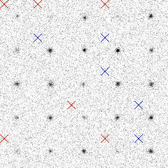
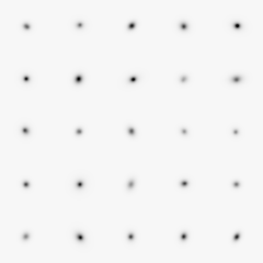
Figure 1: A sample of the target (left) and template (right) simulated galaxies used in the validation test. Targets are marked here with an X in the upper left of their stamp if they were cut for low (red) or high (blue) $S/N$.

The range of flux assigned to galaxies is set such that it yields $5<S/N<25$ for a circular galaxy of typical size under matched-aperture detection. In measuring shear, we set selection bounds $f_{\rm min}=8\sigma_{f},f_{\rm max}=20\sigma_{f}$. Note that the selection uses a different definition of $S/N$ than the generation. At fixed flux, the selection favors more compact and more circular galaxies.

The properties for these simulated galaxies were chosen to capture the non-idealities of real data which might affect the BFD implementation:

• We give the PSF an ellipticity $e_{2}=0.05$, which will test our ability to reject PSF asymmetries.

• The Moffat PSF is not strictly band-limited so the data are slightly aliased. The PSF half-light radius of 1.5 pixels yields a sampling equivalent to DES imaging in seeing with FWHM of 0$\farcs$8, which would be in the worst-sampled quartile of the data.

• The decentering of the disk and bulge components breaks the perfect elliptical symmetry of the galaxies, which might otherwise be canceling some systematic error in the method.

• Elliptical Gaussians are a six-parameter family, and hence a given point in the 6d $(\mbox{\boldmath$M$}^{G},\mbox{\boldmath$X$}^{G})$ space has only a single possible value for the shear derivatives. The varying bulge fraction and bulge/disk misregistration in the GalSim simulations admit a range of shear derivatives at each point in moment space.

• These tests include a non-trivial selection function and hence test the validity of the BFD terms for non-selection.

We produce a total of f which a fraction 0.69105 pass the flux selection test. The calculated $P(s)$ from Equation (40) predicts this extremely well: $0.69111\pm 0.00006$. The uncertainty on $P(s)$ arises from sampling noise in the template set.

Most importantly, the inferred values for $g_{1}$ and $g_{2}$ imply

$$m =c$$