Flocking and non-flocking behavior in a stochastic Cucker-Smale system

Abstract.

We first present a new stochastic version of the Cucker-Smale model of the emergent behavior in flocks in which the mutual communication between individuals is affected by random factor. Then, the existence and uniqueness of global solution to this system are verified. We show a result which agrees with natural fact that under the effect of large noise, there is no flocking. In contrast, if noise is small, then flocking may occur. Paper ends with some numerical examples.

1. Introduction

Flocking is a prevalent behavior of most population in natural world such as bacteria, birds, fishes. It is also widespread in some phenomena in physics, for example interacting oscillators. Recently, a number of articles proposed mathematical models for flocking behavior, to name a few [4, 5, 7, 12, 15, 16, 17, 18]. Vicsek and collaborators [18] presented a model (for convenience, we call it Vicsek’s model) and then studied flocking behavior via computer simulations. Some theoretical results on the convergence of that model can be found in [15]. Based on the Vicsek’s model, Cucker and Smale introduced a model for an $N$-particle system [4, 5]. Then, some mathematicians called it the Cucker-Smale system [1, 3, 10, 11, 13, 17]. We will recall here some features of this system. We consider motion of $N$ particles in the space $\mathbb{R}^{d}\,(d=1,2,3,\ldots)$. The position of the $i$-th particle is denoted by $x_{i}=x_{i}(t)\,(i=1,2,\ldots,N)$. Its velocity is denoted by $v_{i}=v_{i}(t)\,(i=1,2,\ldots,N)$. The Cucker-Smale system is as follows

$$\begin{cases}x_{i}^{\prime}=v_{i},\hskip 85.35826pt1\leq i\leq N,\\ v_{i}^{\prime}=\frac{1}{N}\sum_{j=1}^{N}\psi(||x_{j}-x_{i}||)(v_{j}-v_{i}),\end{cases}$$ (1.1)

Here, the weights $\psi(||x_{j}-x_{i}||)$ quantify the influence between $i$-th and $j$-th particles. This communication rate is a nonincreasing function $\psi\,{:}\,[0,\infty)\rightarrow[0,\infty)$ of the distances between particles. This function has various forms. In [4, 5], $\psi(s)=\frac{K}{(c+s^{2})^{\beta}},$ while in [11, 13], $\psi(s)=\frac{K}{(c+s^{2})^{\beta}}$, $\psi(s)=\frac{K}{s^{2\beta}}$ or $\psi(s)=\text{\rm constant}$. For such functions, it is shown that when $\beta<\frac{1}{2}$ the convergence of the velocities to a common velocity is guaranteed, while for $\beta\geq\frac{1}{2}$ this convergence is guaranteed under some condition on the initial positions and velocities of particles. We call them unconditional flocking and conditional flocking, respectively. In the latter case, the result on the non-flocking for two particles on a line is also stated [5].

We know that real systems are often exposed to influences that are incompletely understood. Therefore extending these deterministic models to ones that embrace more complicated variations is needed. A way of doing that is including stochastic influences or noise. Up to our knowledge, however, there are few such models which are studied theoretically [6, 13, 1]. In [6], Cucker and Mordecki modified the model (1.1) in $\mathbb{R}^{3}$ by adding random noise to it

$$\begin{cases}x_{i}^{\prime}=v_{i},\hskip 85.35826pt1\leq i\leq N,\\ v_{i}^{\prime}=\sum_{j=1}^{N}\psi(||x_{j}-x_{i}||)(v_{j}-v_{i})+H_{i},\end{cases}$$ (1.2)

Here communication rate $\psi$ has the same form as that in (1.1). $H_{i}(t)$ is a three-dimensional Gausian centered, stationary stochastic process, that satisfies a $\delta$ - dependence condition for some $\delta>0$, i.e., two sets $\{H_{i}(s)|s\leq t\}$ and $\{H_{i}(s)|s\geq t+\delta\}$ are independent for each $t$. And $H_{i}(t)$ has $\mathcal{C}^{0}$ trajectories and independent coordinates. The authors showed that a conditional $\nu$ - nearly flocking occurs in finite time with a confidence which is similar to the conditional flocking of the deterministic system (1.1). That is, for $\nu>0$ small enough, there exists a time $T_{0}$ depending on $\nu$ and initial values $v_{i}(0)\,(1\leq i\leq N)$ such that for every $t\in[0,T_{0})$, $\sum_{i,j}||v_{i}(t)-v_{j}(t)||\leq\nu$ with a positive probability. This probability, however, is not one and the interval time for the occurring is not $[0,\infty)$. In other words, it is just nearly flocking, not flocking. In another approach, Ha and collaborators [13, 1] studied the following two Cucker-Smale systems with the presence of white noise:

$$\begin{cases}dx_{i}=v_{i}dt,\hskip 85.35826pt1\leq i\leq N,\\ dv_{i}=\frac{\lambda}{N}\sum_{j=1}^{N}\psi(||x_{j}-x_{i}||)(v_{j}-v_{i})dt+\sqrt{D}dw_{i},\end{cases}$$ (1.3)

and

$$\begin{cases}dx_{i}=v_{i}dt,\hskip 85.35826pt1\leq i\leq N,\\ dv_{i}=\frac{\lambda}{N}\sum_{j=1}^{N}\psi(||x_{j}-x_{i}||)(v_{j}-v_{i})dt+D(v_{i}-v_{e})dw_{i},\end{cases}$$ (1.4)

where $v_{e}$ is a constant vector. In [13], the result on the flocking behavior of system (1.3) is exhibited when the communication rate is a constant. Furthermore, if the communication rate satisfies a lower bound condition, then the relative fluctuations of velocities around a mean velocity have a uniformly bounded variance in time. In [1], by giving another definition for flocking which is relative to almost surely convergence, the authors showed flocking of system (1.4) which covers the case of the communication weight employed by Cucker-Smale.

We are interested in the communication rate term in system (1.1). What happens if this mutual communication is affected by random factor, i.e., $\psi(|x_{j}-x_{i}|)\leadsto\psi(|x_{j}-x_{i}|)$ + white noise? This motivates us to present and study a Cucker-Smale system under the effect of a common white noise on the mutual communication. We will show that if the noise is large then there is no flocking. Even if the communication rate satisfies the unconditional flocking for (1.1), this still holds true. This is different from the deterministic Cucker-Smale system (1.1) but is adaptive to real situations. For example, under a strongly random effect of strong winds or water currents, birds or fishes will separate and can not make a flock or school. In contrast, we will show that if the noise is small enough, then flocking occurs. For the convenience of calculation, we will use the Stratonovich stochastic differential equations. Our model to study in this paper has the form

$$\begin{cases}dx_{i}=v_{i}dt,\\ \hskip 284.52756pt1\leq i\leq N.\\ dv_{i}=\sum_{j=1}^{N}\psi(||x_{j}-x_{i}||)(v_{j}-v_{i})dt+\sigma\sum_{j=1}^{N}(v_{j}-v_{i})\circ dw_{t},\end{cases}$$ (1.5)

Here $\sigma>0$ is the strength of white noise and $\{w_{t},t\geq 0\}$ is one-dimensional Brownian motion defined on a complete probability space with normal filtration $(\Omega,\mathcal{F},\{\mathcal{F}_{t}\}_{t\geq 0},\mathbb{P})$. We assume that communication rate function $\psi\,{:}\,[0,\infty)\rightarrow[0,\infty)$ is locally Lipschitz continuous.

The organization of the paper is as follows. In the next section, we prove the existence and uniqueness of global solution to (1.5). In Section 3, non-flocking under the effect of large noise is shown. In contrast, in Section 4, we exhibit flocking under the effect of small noise. Finally, some numerical examples are presented in Section 5.

2. Existence and uniqueness of global solution

In this section, we shall prove global existence of solution for the system (1.5).

Theorem 2.1.

For any given initial values $(x_{i}(0),v_{i}(0))\in\mathbb{R}^{2d}\,(1\leq i\leq N),$ system (1.5) has a unique and global solution.

Proof.

Since the functions on the right side of (1.5) are locally Lipschitz continuous on $\mathbb{R}^{2d},$ there is a unique solution $(x_{i}(t),v_{i}(t))\,(1\leq i\leq N)$ defined on an interval $[0,\tau),$ where $\tau\leq\infty$ and if $\tau<\infty$ it is an explosion time [2, 8], i.e.,

$$\tau=\sup\{t\,{:}\,\sup_{s\in[0,t),1\leq i\leq N}[||x_{i}(s)||+||v_{i}(s)||]<\infty\}.$$

Put

$$||x||=\sqrt{\sum_{i=1}^{N}||x_{i}||^{2}},\quad||v||=\sqrt{\sum_{i=1}^{N}||v_{i}||^{2}},\quad\bar{x}=\frac{1}{N}\sum_{i=1}^{N}x_{i},\quad\bar{v}=\frac{1}{N}\sum_{i=1}^{N}v_{i}.$$

It follows from system (1.5) that

$$\begin{cases}d\bar{x}=\bar{v}dt,\\ d\bar{v}={\bf 0}.\end{cases}$$

Then almost surely $\bar{x}(t)=\bar{x}(0)+\bar{v}(0)t$ and $\bar{v}(t)=\bar{v}(0)$ for every $t\in[0,\tau).$ Without loss of generality, we may assume that $\bar{x}(0)=\bar{v}(0)={\bf 0}$. Then,

$$\sum_{i=1}^{N}x_{i}(t)=\sum_{i=1}^{N}v_{i}(t)={\bf 0}\hskip 56.9055pt\text{ a.s.}$$ (2.1)

and

$$\sum_{i,j=1}^{N}||v_{i}(t)-v_{j}(t)||^{2}=2N||v(t)||^{2}.$$ (2.2)

It follows from the second equation of (1.5) and from the chain rule of Stratonovich stochastic differential equation that

$$d||v||^{2}= \sum_{i=1}^{N}d||v_{i}||^{2}$$ (2.3)

$$= 2\sum_{i=1}^{N}<v_{i},dv_{i}>$$

$$= 2\sum_{i,j=1}^{N}\psi(||x_{j}-x_{i}||)<v_{i},v_{j}-v_{i}>dt+2\sigma\sum_{i,j=1}^{N}<v_{i},v_{j}-v_{i}>\circ dw_{t}.$$

We have

$$\sum_{i,j=1}^{N}<v_{i},v_{j}-v_{i}> =\sum_{i,j=1}^{N}<v_{i}-v_{j},v_{j}-v_{i}>+\sum_{i,j=1}^{N}<v_{j},v_{j}-v_{i}>$$

$$=-\sum_{i,j=1}^{N}||v_{i}-v_{j}||^{2}-\sum_{i,k=1}^{N}<v_{k},v_{i}-v_{k}>,$$

which induces

$$2\sum_{i,j=1}^{N}<v_{i},v_{j}-v_{i}> =-\sum_{i,j=1}^{N}||v_{i}-v_{j}||^{2}$$

$$=-2N||v||^{2}\quad(\text{ see }\eqref{E7}).$$ (2.4)

Furthermore, it follows from

$$\sum_{i,j=1}^{N}\psi(||x_{j}-x_{i}||)<v_{i},v_{j}-v_{i}>= -\sum_{i,j=1}^{N}\psi(||x_{j}-x_{i}||)||v_{i}-v_{j}||^{2}$$

$$+\sum_{i,j=1}^{N}\psi(||x_{j}-x_{i}||)<v_{j},v_{j}-v_{i}>$$

that

$$2\sum_{i,j=1}^{N}\psi(||x_{j}-x_{i}||)<v_{i},v_{j}-v_{i}>=-\sum_{i,j=1}^{N}\psi(||x_{j}-x_{i}||)||v_{i}-v_{j}||^{2}.$$ (2.5)

Thus, by (2.3)-(2.5), we obtain

$$d||v||^{2}=-\sum_{i,j=1}^{N}\psi(||x_{j}-x_{i}||)||v_{i}-v_{j}||^{2}dt-2N\sigma||v||^{2}\circ dw_{t}.$$

Or, equivalently, in the Itô form:

$$d||v||^{2}=\left[-\sum_{i,j=1}^{N}\psi(||x_{j}-x_{i}||)||v_{i}-v_{j}||^{2}+2N^{2}\sigma^{2}||v||^{2}\right]dt-2N\sigma||v||^{2}dw_{t}.$$ (2.6)

Hence, by using the comparison theorem [14], it follows from (2.6) that for every $t\geq 0$, $||v(t)||^{2}\leq V(t)$ a.s., where $V(t)$ satisfies the following equation

$$\begin{cases}dV=2N^{2}\sigma^{2}Vdt-2N\sigma Vdw_{t},\\ V(0)=||v(0)||^{2}.\end{cases}$$

This linear equation has a unique global solution $V(t)=V(0)e^{-2N\sigma w_{t}}.$ Thus for every $t\in[0,\tau)$

$$||v(t)||\leq||v(0)||e^{-N\sigma w_{t}}\hskip 56.9055pt\text{a.s. }$$ (2.7)

Then, from the first equation of (1.5) we have almost surely

$$d||x||^{2} =\sum_{i=1}^{N}d||x_{i}||^{2}=2\sum_{i=1}^{N}<x_{i},v_{i}>dt$$

$$\leq 2||x||\,||v||dt\leq 2||v(0)||e^{-N\sigma w_{t}}||x||dt.$$

By the comparison theorem, we obtain $||x(t)||^{2}\leq X(t)$ for all $t\geq 0$, where $X(t)$ satisfies the following equation

$$\begin{cases}dX=2||v(0)||e^{-N\sigma w_{t}}\sqrt{X}dt,\\ X(0)=||x(0)||^{2}>0.\end{cases}$$

Since $X(t)=[||x(0)||+||v(0)||\int_{0}^{t}e^{-N\sigma w_{s}}ds]^{2},$ then for every $t\in[0,\tau)$

$$||x(t)||\leq||x(0)||+||v(0)||\int_{0}^{t}e^{-N\sigma w_{s}}ds\hskip 56.9055pt\text{ a.s.}$$ (2.8)

From (2.7), (2.8) and the definition of $\tau$, we see that $\tau=\infty$ a.s. It means that the solution to (1.5) is unique and global. ∎

3. Non-flocking under large noise

In this section, we will show that under the effect of large noise on particles, i.e., $\sigma$ is large, then the system (1.5) does not flock. First, we give a definition for flocking. Then non-flocking theorem is shown.

Definition 3.1.

The state of particles $(x_{i}(t),v_{i}(t))\,(1\leq i\leq N)$ in system (1.5) has a time-asymptotic flocking if, for $1\leq i,j\leq N$, the velocity alignment and group forming in the following senses, respectively, are satisfied

• $\lim_{t\to\infty}\mathbb{E}||v_{i}-v_{j}||^{2}=0.$

• $\sup_{0\leq t<\infty}\mathbb{E}||x_{i}-x_{j}||<\infty.$

Put $\alpha=\sup_{s\geq 0}\psi(s).$ Throughout this section, we assume that the communication rate satisfies an upper bound condition, i.e., $\alpha<\infty$. Note that the communication rate in Cucker-Smale system [4, 5] satisfies this condition.

Theorem 3.2 (Non-flocking theorem).

If $\sigma>\sqrt{\frac{\alpha}{N}}$ then the particles do not flock.

Proof.

As we see in the proof of Theorem 2.1 that without loss of generality, we can assume that $\bar{x}(0)=\bar{v}(0)={\bf 0}.$ Then (2.1) and (2.2) hold true. It follows from (2.2) and (2.6) that

$$d||v||^{2}= \sum_{i,j=1}^{N}[N\sigma^{2}-\psi(||x_{j}-x_{i}||)]||v_{i}-v_{j}||^{2}dt-2N\sigma||v||^{2}dw_{t}$$

$$\geq \sum_{i,j=1}^{N}(N\sigma^{2}-\alpha)||v_{i}-v_{j}||^{2}dt-2N\sigma||v||^{2}dw_{t}$$

$$= 2N(N\sigma^{2}-\alpha)||v||^{2}dt-2N\sigma||v||^{2}dw_{t}.$$

By using the comparison theorem, for every $t\geq 0$ we have $||v(t)||^{2}\geq V_{1}(t)$ a.s., where $V_{1}(t)$ is a unique solution of the following equation

$$\begin{cases}dV_{1}=2N(N\sigma^{2}-\alpha)V_{1}dt-2N\sigma V_{1}dw_{t},\\ V_{1}(0)=||v(0)||^{2}>0.\end{cases}$$

Since $d\mathbb{E}V_{1}=2N(N\sigma^{2}-\alpha)\mathbb{E}V_{1}dt,$ we have $\mathbb{E}V_{1}(t)=||v(0)||^{2}e^{2N(N\sigma^{2}-\alpha)t}\rightarrow\infty$ as $t\rightarrow\infty$. Therefore, $\mathbb{E}||v(t)||^{2}\rightarrow\infty$ as $t\rightarrow\infty$. It means that the particles do not flock. ∎

4. Flocking under small noise

In this section, we consider the system (1.5) under the effect of small noise, i.e., $\sigma$ is small. We will show that flocking takes place under a lower bound condition of the communication rate.

Theorem 4.1 (Flocking theorem).

Assume that there exists $\psi^{*}>0$ such that

$$\inf_{s\geq 0}\psi(s)\geq\psi^{*}.$$

If $\sigma<\sqrt{\frac{\psi^{*}}{N}}$ then particles flock under any initial values $(x_{i}(0),v_{i}(0))\in\mathbb{R}^{2d}\,(1\leq i\leq N)$.

Proof.

Similar to Theorem 3.2, we can assume that $\bar{x}(0)=\bar{v}(0)={\bf 0}.$ Then (2.1) and (2.2) hold true. By (2.2) and (2.6), we have

$$d||v||^{2}\leq \left[-\sum_{i,j}^{N}\psi^{*}||v_{i}-v_{j}||^{2}+2N^{2}\sigma^{2}||v||^{2}\right]dt-2N\sigma||v||^{2}dw_{t}$$

$$= \big{(}N\sigma^{2}-\psi^{*}\big{)}||v||^{2}dt-2N\sigma||v||^{2}dw_{t}.$$

By using the comparison theorem, it follows that $||v(t)||^{2}\leq V_{2}(t)$ a.s., where $V_{2}(t)$ satisfies the following equation

$$\begin{cases}dV_{2}=\big{(}N\sigma^{2}-\psi^{*}\big{)}V_{2}dt-2N\sigma V_{2}dw_{t},\\ V_{2}(0)=||v(0)||^{2}.\end{cases}$$ (4.1)

Since $d\mathbb{E}V_{2}=\big{(}N\sigma^{2}-\psi^{*}\big{)}\mathbb{E}V_{2}dt$ and $\sigma<\sqrt{\frac{\psi^{*}}{N}},$ we have

$$\mathbb{E}||v(t)||^{2}\leq EV_{2}(t)=||v(0)||^{2}e^{(N\sigma^{2}-\psi^{*})t}\rightarrow 0\text{ as }t\rightarrow\infty.$$

On the other hand, the linear equation (4.1) has an explicit solution

$$V_{2}(t)=||v(0)||^{2}e^{[(N-2N^{2})\sigma^{2}-\psi^{*}]t-2N\sigma w_{t}}.$$

Thus,

$$||v(t)||\leq||v(0)||e^{\frac{1}{2}\big{[}(N-2N^{2})\sigma^{2}-\psi^{*}\big{]}t-N\sigma w_{t}}.$$ (4.2)

In the prove of Theorem 2.1, we showed that $d||x||^{2}\leq 2||x||||v||dt$. Then by using the comparison theorem and (4.2), it is easy to obtain that

$$||x(t)||\leq||x(0)||+||v(0)||\int_{0}^{t}e^{\frac{1}{2}[(N-2N^{2})\sigma^{2}-\psi^{*}]s-N\sigma w_{s}}ds.$$

Thus,

$$\mathbb{E}||x(t)||\leq ||x(0)||+||v(0)||\int_{0}^{t}e^{\frac{1}{2}[(N-2N^{2})\sigma^{2}-\psi^{*}]s}\mathbb{E}e^{-N\sigma w_{s}}ds$$

$$= ||x(0)||+||v(0)||\int_{0}^{t}e^{\frac{1}{2}[(N-2N^{2})\sigma^{2}-\psi^{*}]s}e^{\frac{1}{2}N^{2}\sigma^{2}s}ds$$

$$= ||x(0)||+||v(0)||\int_{0}^{t}e^{\frac{1}{2}[(N-N^{2})\sigma^{2}-\psi^{*}]s}ds$$

$$= ||x(0)||+||v(0)||\frac{2}{(N-N^{2})\sigma^{2}-\psi^{*}}\left[e^{\frac{1}{2}[(N-N^{2})\sigma^{2}-\psi^{*}]t}-1\right].$$

Therefore, $\sup_{t\geq 0}\mathbb{E}||x(t)||<\infty.$ From the above results, we conclude that the particles flock. ∎

Remark 4.2.

The lower bound condition has been used for the system (1.3) by Ha et al. [13]. The authors showed that when this condition holds true, the term $\mathbb{\sum}_{i,j}E||v_{i}-v_{j}||^{2}$ is uniformly bounded in $t.$ Furthermore, when $\psi=1$, flocking of particles takes place. However, when $\psi$ satisfies the lower bound condition but is not a constant, the flocking result has not yet obtained in [13].

Remark 4.3.

The above flocking result is relative to the expectation (average) of solution. We can obtain a result on flocking of almost surely convergence that is valid for individual trajectory. To see that, firstly, we change the first condition in Definition 3.1 by $\lim_{t\to\infty}||v_{i}-v_{j}||=0$ a.s. Now, it follows from (4.2) that

$$||v(t)||\leq||v(0)||e^{t\big{[}\frac{1}{2}(N-2N^{2})\sigma^{2}-\psi^{*}-N\sigma\frac{w_{t}}{t}\big{]}}.$$ (4.3)

By the strong law of large numbers for Brownian motion [9], $\frac{w_{t}}{t}\rightarrow 0$ as $t\rightarrow\infty$ a.s. Thus $\lim_{t\to\infty}||v(t)||=0.$ It then follows from (2.2) that for $1\leq i\leq N$,

$$\lim_{t\to\infty}||v_{i}-v_{j}||=0\hskip 56.9055pt\text{ a.s.}$$ (4.4)

It means that flocking occurs. Furthermore, it is easy to see from (4.3) that (4.4) still holds true for the case $\sigma>0,\psi^{*}=0$. This means that flocking occurs without the assumptions on the positivity of $\psi^{*}$ and upper boundedness of $\sigma$. Consequently, unconditional flocking occurs not only for the communication rate $\psi$ in [13] but for those in [4, 5, 6].

5. Numerical examples

In this section, we present some results of numerical simulations based on Euler’s method for the system (1.5). First, we give examples for non-flocking, second, examples for flocking.

5.1. Non-flocking

Let us first observe an example that shows that the system (1.5) does not flock.

Set $\alpha=1,\sigma=0.3$ and $\psi(s)=\frac{\alpha}{(1+s^{2})^{0.25}}$. We compute $100$ trajectories of solution of (1.5) in $\mathbb{R}^{2}$ with $N=50$ and initial values $(x_{i}(0),v_{i}(0))$ are randomly generated in $[0,0.1]^{4}$. Figure 1 illustrates behavior of function $f(t)=\sum_{i<j}\mathbb{E}||v_{i}(t)-v_{j}(t)||^{2}$ up to time $T=0.2.$ We see that values of function $f(t)$ are very large even at small time $t$.

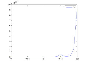
Figure 1. Non-flocking in $2$-dim. space

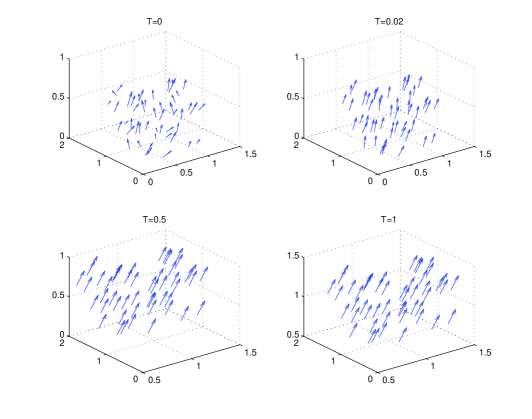
Figure 2. Flocking in $3$-dim. space

5.2. Flocking

Let us next observe another example showing flocking. Set $\alpha=1,\sigma=0.05$ and $\psi(s)=1.$ Initial values $(x_{i}(0),v_{i}(0))$ are generated randomly in $[0,1]^{6}$. Figure 2 shows a flock of $50$ particles at $T=0,0.02,0.5,1$. Each vector shows position and direction of motion of each particle. The lengths of vectors represent the magnitudes of velocity vectors of particles.

6. Conclusion

This paper presented a new stochastic version of the Cucker-Smale model in which the mutual communication between individuals is affected by the common random factor. This model can find its applications in real world because almost every real phenomena are subject to environmental noises. Under the upper bound condition of communication rate, we show that if the noise is large then the particles can not flock. This is consistent with some situations in nature, for example, under a strongly random effect, there is no flock. In contrast, under the lower bound condition of communication rate and small noise, flocking occurs. The paper ends with some numerical examples of both flocking and non-flocking.

Using the sense of flocking stated in Remark 4.3, unconditional flocking takes place. However, a remaining interesting problem for the stochastic Cucker-Smale model is to obtain flocking results in the sense of Definition 3.1. By numerical simulations, we predict that flocking in this case does not only depend on small noise but on some certain domain of initial values $(x_{i}(0),v_{i}(0)).$ This problem is left for our future research.

References

- [1] S. M. Ahn, S. -Y. Ha, Stochastic flocking dynamics of the Cucker-Smale model with multiplicative white noises, J. Math. Phys. 51 (2010), 103301.
- [2] L. Arnold, Stochastic Differential Equations: Theory and Applications (Wiley, New York, 1972).
- [3] J. A. Carrillo, M. Fornasier, J. Rosado, G. Toscani, Asymptotic flocking dynamics for the kinetic Cucker-Smale model, SIAM J. Math. Anal. 42 (2010), 218-236.
- [4] F. Cucker, S. Smale, On the mathematics of emergence, Japan. J. Math. 2 (2007), 197-227.
- [5] F. Cucker, S. Smale, Emergence behavior in flocks, IEEE Trans. Automat. Control 52 (2007), 852-862.
- [6] F. Cucker, E. Mordecki, Flocking in noisy environments, J. Math. Pures Appl. 89 (2008), 278-296.
- [7] G. Flierl, D. Grünbaum, S. Levin, and D. Olson, From individuals to aggregations: The interplay between behavior and physics, J. Theor. Biol. 196 (1999), 397-454.
- [8] A. Friedman, Stochastic Differential Equations and their Applications (Academic press, New York, 1976).
- [9] I. Karatzas, S. E. Shreve, Brownian Motion and Stochastic Calculus (Springer-Verlag, Berlin, 1991).
- [10] S. Motsch, E. Tadmor, A new model for self-organized dynamics and its flocking behavior, J. Stat. Phys. 144 (2011), 923-947.
- [11] S. -Y. Ha, J. Liu, A simple proof of the Cucker-Smale flocking dynamics and mean-field limit, Commun. Math. Sci. 7(2) (2009), 297-325.
- [12] S. -Y. Ha, E. Tadmor, From particle to kinetic and hydrodynamic descriptions of flocking, Kinet. Relat. Models 1 (2008), 415-435.
- [13] S. -Y. Ha, K. Lee, D. Levy, Emergence of time-asymptotic flocking in a stochastic Cucker-Smale system, Commun. Math. Sci. 7(2) (2009), 453-469.
- [14] N. Ikeda, S. Wantanabe. Stochastic Differential Equations and Diffusion Processes (North-Holland, Amsterdam, 1981).
- [15] A. Jadbabaie, J. Lin, and A. Morse, Coordination of groups of mobile autonomous agents using nearest neighbor rules, IEEE Trans. Automat. Control 48 (2003), 988-1001.
- [16] R. Olfati-saber, Flocking for multi-agent dynamic systems: Algorithms and theory, IEEE Trans. Automat. Control 51 (2006), 401-420.
- [17] J. Shen, Cucker-Smale flocking under hierarchical leadership, SIAM J. Appl. Math. 68 (2007), 694-719.
- [18] T. Vicsek, A. Czirók, E. Ben-Jacob, and O. Shochet, Novel type of phase transition in a system of self-driven particles, Phys. Rev. Lett. 75 (1995), 1226-1229.