Population annealing: Theory and application in spin glasses

Abstract

Population annealing is an efficient sequential Monte Carlo algorithm for simulating equilibrium states of systems with rough free energy landscapes. The theory of population annealing is presented, and systematic and statistical errors are discussed. The behavior of the algorithm is studied in the context of large-scale simulations of the three-dimensional Ising spin glass and the performance of the algorithm is compared to parallel tempering. It is found that the two algorithms are similar in efficiency though with different strengths and weaknesses.

I Introduction

One of the most difficult challenges faced in computational physics is simulating the equilibrium states of disordered systems with rough free energy landscapes, such as spin glasses Binder and Young (1986); Stein and Newman (2013). Standard Markov-chain Monte Carlo methods operating at a single temperature, such as the Metropolis algorithm, equilibrate extremely slowly at low temperatures due to trapping in metastable states. Algorithms that make use of simulations at many temperatures partially solve this problem and are now the methods of choice for equilibrium simulations of disordered systems with frustration. Markov-chain Monte Carlo methods in this general category include parallel tempering Monte Carlo Swendsen and Wang (1986); Geyer (1991); Hukushima and Nemoto (1996); Earl and Deem (2005); Katzgraber et al. (2006a), simulated tempering Monte Carlo Marinari and Parisi (1992), and the Wang-Landau algorithm Wang and Landau (2001a, b). Population annealing Monte Carlo Hukushima and Iba (2003); Machta (2010); Machta and Ellis (2011), the topic of this paper, is an alternative to these multicanonical algorithms. Population annealing also employs many temperatures. However, it is not a Markov-chain Monte Carlo method. Instead, population annealing is a sequential Monte Carlo method Doucet et al. (2001). Population annealing was introduced by Hukushima and Iba Hukushima and Iba (2003) and further developed in Refs. Machta (2010) and Machta and Ellis (2011). The algorithm was independently discovered and called “sequential Monte Carlo simulated annealing” in Ref. Zhou and Chen (2010). Sequential Monte Carlo algorithms are not commonly used in computational physics. However, the approach has been applied to some problems, e.g., the diffusion Monte Carlo method for finding ground states of many-body Schrodinger equations and Grassberger’s “Go with Winners” method Grassberger (2002).

Population annealing has been successfully used in large-scale simulations of Ising spin glasses by the present authors Wang et al. (2014, 2015a). One of the purposes of this paper is to give additional details of the implementation and performance of the population annealing algorithm as used in Refs. Wang et al. (2014) and Wang et al. (2015a). We have also successfully used population annealing as a heuristic to find spin-glass ground states Wang et al. (2015b) and have shown that population annealing is comparably efficient to parallel tempering Monte Carlo while both are far more efficient than simulated annealing Kirkpatrick et al. (1983). The current state-of-the-art algorithm for simulations of spin glasses and related systems with rough free-energy landscapes is parallel tempering Monte Carlo. Another purpose of this paper to argue that population annealing is a useful alternative and potentially superior to parallel tempering for large-scale studies of the equilibrium properties of spin glasses and other disordered systems. We carry out a detailed comparison of population annealing and parallel tempering for simulating spin glasses and we find that the two methods are comparably efficient for sampling thermal states, although each method has advantages and disadvantages. We also develop a theory that quantifies the rate of convergence to equilibrium of population annealing and compare the theoretical predictions to simulations.

The outline of the paper is as follows. In Sec. II we introduce both population annealing and parallel tempering Monte Carlo, and in Sec. III we discuss several features of population annealing. Section IV is concerned with the systematic and statistical errors in population annealing and the section concludes with a comparison of errors to those in Markov chain Monte Carlo methods such as parallel tempering. Section V introduces the Edwards-Anderson Ising spin glass model and gives details of the simulations and the quantities that were measured. Section VI presents the results of large-scale simulations using both population annealing and parallel tempering with an emphasis on elucidating the properties of population annealing and comparing them to parallel tempering. The paper concludes with a discussion in Sec. VII

II Population Annealing and Parallel Tempering Monte Carlo

II.1 Population annealing

Population annealing (PA) is closely related to simulated annealing Kirkpatrick et al. (1983) (SA) except that it uses a population of replicas and this population is resampled at each temperature step. Like simulated annealing, PA involves lowering the temperature of the system through a sequence of temperatures from a high temperature where equilibration (also known as thermalization) is easy to a low, target temperature $T_{0}$ where equilibration is difficult. Unlike SA, PA is designed to simulate the equilibrium Gibbs distribution at each temperature that is traversed. The resampling step ensures that the population stays close to the equilibrium ensemble. Just as in simulated annealing, at each temperature, each replica is acted on by a Markov-chain Monte Carlo (MCMC) procedure such as the Metropolis algorithm. The annealing schedule consists of a sequence $\{\beta_{N_{T}-1},\ldots,\beta_{0}\}$ of $N_{T}$ inverse temperatures, $\beta=1/T$ labeled in descending order in $\beta$ so that $\beta_{j+1}<\beta_{j}$. In our studies, the inverse temperatures are equally spaced, starting at infinite temperature, $\beta_{N_{T}-1}=0$ and ending at $\beta_{0}=5$. The MCMC method is the Metropolis algorithm Metropolis and Ulam (1949); Metropolis et al. (1953), which is applied for $N_{S}$ sweeps at each temperature. The initial population size is $R$ and each replica is independently initialized with random spins corresponding to an infinite temperature ensemble. In our implementation the population size fluctuates. In a given run at inverse temperature $\beta$ the population size is $\tilde{R}_{\beta}$ with a mean value of $R$.

The resampling step uses differential reproduction of replicas with a number of copies depending on the replica’s energy. Let $E_{j}$ be the energy of replica $j$. Given an equilibrium population at $\beta$, the goal is to resample the population so that it is an equilibrium population at $\beta^{\prime}$ with $\beta^{\prime}>\beta$. For a replica $j$, with energy $E_{j}$ the ratio of the statistical weights at $\beta$ and $\beta^{\prime}$ is $\exp\left[-(\beta^{\prime}-\beta)E_{j}\right]$. Note that this is the reweighting used in the histogram re-weighting method Ferrenberg and Swendsen (1988).

Since the typical energy is large and negative, the reweighting factor is much greater than unity so that a normalization is needed to keep the population size close to $R$. The normalized weights $\tau_{j}(\beta,\beta^{\prime})$ are given by,

$$\tau_{j}(\beta,\beta^{\prime})=\frac{R}{\tilde{R}_{\beta}}\cdot\frac{e^{-(\beta^{\prime}-\beta)E_{j}}}{Q(\beta,\beta^{\prime})},$$ (1)

where $Q(\beta,\beta^{\prime})$ is the normalization,

$$Q(\beta,\beta^{\prime})=\frac{1}{\tilde{R}_{\beta}}\sum_{j=1}^{\tilde{R}_{\beta}}e^{-(\beta^{\prime}-\beta)E_{j}}.$$ (2)

Note that the sum of $\tau_{j}(\beta,\beta^{\prime})$ over $j$ is $R$.

The new population at temperature $\beta^{\prime}$ is obtained by resampling the old population such that the number of copies $n_{j}$ of replica $j$ is a random non-negative integer whose mean is $\tau_{j}(\beta,\beta^{\prime})$. There are many ways to choose $n_{j}$ to satisfy this requirement Douc and Cappe (2005). Some of these methods such as a multinomially distributed $n_{j}$ keep the population size fixed while others allow the population size to fluctuate. We choose a method that minimizes the variance of $n_{j}$ and has $\sqrt{R}$ fluctuations in the population size. Let $n_{j}$ be $\lfloor\tau_{j}\rfloor$ with probability $1-(\tau_{j}-\lfloor\tau_{j}\rfloor)$ or $\lceil\tau_{j}\rceil$ with probability $(\tau_{j}-\lfloor\tau_{j}\rfloor)$ where $\lfloor\tau_{j}\rfloor$ is the floor (greatest integer less than) $\tau_{j}$ and $\lceil\tau_{j}\rceil$ is the ceiling (least integer greater than) $\tau_{j}$. By minimizing the variance of $n_{j}$ we reduce correlations in the population while the fluctuating population size creates a small overhead in memory usage.

Consider a single temperature step in PA. If the original, higher temperature population is an equilibrium ensemble representing the Gibbs distribution at inverse temperature $\beta$ then the final, lower temperature population is also an equilibrium ensemble at inverse temperature $\beta^{\prime}$. However, the new population is correlated due to copying replicas in the resampling step and, for finite $R$, the new population represents a biased ensemble due to a lack of representation of the low energy tail of the $\beta^{\prime}$ Gibbs distribution. These errors are partially corrected by the MCMC sweeps $\beta^{\prime}$. Statistical and systematic errors are discussed in Sec. IV.

The full PA algorithm is a sequence of $N_{T}-1$ annealing steps starting from infinite temperature. In each annealing step the population is resampled and then $N_{S}$ sweeps of the Metropolis algorithm are carried out on each replica.

II.2 Parallel Tempering

In this section, we briefly describe parallel tempering (PT) Monte Carlo, the state-of-the-art Monte Carlo algorithm for spin glasses and many other frustrated systems. Parallel tempering is a Markov-chain Monte Carlo algorithm while population annealing is a sequential Monte Carlo algorithm, nonetheless, the two algorithms share many similarities. In parallel tempering, a set of $N_{T}$ temperatures is used ranging from a high temperature that is easy to equilibrate to a low temperature of interest, $T_{0}$. There is a single replica of the system at each of these temperatures and each of these replicas is operated on by a MCMC method such as the Metropolis algorithm at that temperature. After $N_{S}$ sweeps of the replicas at their respective temperatures, replica exchange moves are proposed. In a replica exchange move, replicas at two temperatures are proposed for swapping. Typically, the two temperatures are chosen to be neighboring temperatures in the list of temperatures. Let these two inverse temperatures be $\beta$ and $\beta^{\prime}$ with $\beta^{\prime}>\beta$ and let $E$ and $E^{\prime}$ be the respective energies of the replicas at these two temperatures. The swap is accepted with probability $\min\left[1,\exp[(\beta^{\prime}-\beta)(E^{\prime}-E)]\right]$. It is easily shown that this swap probability satisfies detailed balance Hukushima and Nemoto (1996) with respect to the product measure of Gibbs distributions at the $N_{T}$ temperatures so that PT converges to equilibrium at each temperature. Diffusion of replicas from low temperature to high temperature and back, called ‘round trips’ allows PT to surmount barriers in the free energy landscape Katzgraber et al. (2006a); Machta (2009).

III Features of population annealing

III.1 Free energy estimator

The free-energy difference between the highest and lowest temperature is easily measured using population annealing Machta (2010). If the highest temperature is infinity, as is the case in our implementation of the algorithm, then the absolute free energy can be measured. The key idea is that the normalization factor, defined in Eq. (2), is the ratio of the partition functions at the two inverse temperatures $\beta$ to $\beta^{\prime}$. To see this, expand the definition of $Z(\beta^{\prime})$ and replace the resulting average at $\beta$ by its population estimate,

$$\frac{Z(\beta^{\prime})}{Z(\beta)} = \frac{\sum_{\gamma}e^{-\beta^{\prime}E_{\gamma}}}{Z(\beta)}$$ (3)

$$= \sum_{\gamma}e^{-(\beta^{\prime}-\beta)E_{\gamma}}(\frac{e^{-\beta E_{\gamma}}}{Z(\beta)})$$

$$= \langle e^{-(\beta^{\prime}-\beta)E_{\gamma}}\rangle_{\beta}$$

$$\approx \frac{1}{\tilde{R}_{\beta}}\sum_{j=1}^{\tilde{R}_{\beta}}e^{-(\beta^{\prime}-\beta)E_{j}}=Q(\beta,\beta^{\prime}).$$

The summation over $\gamma$ in the first two lines in the above expressions is over all possible spin configurations while the summation in the last line is over the population. Since $F=-T\ln Z$, the estimator of the free energy ${\tilde{F}}$ at each simulated temperature is,

$$-\beta_{k}{\tilde{F}}(\beta_{k})=\sum^{N_{T}-1}_{\ell=k+1}\ln Q(\beta_{\ell},\beta_{\ell-1})+\ln\Omega,$$ (4)

where $\Omega$ is the number of microstates of the systems and $\{\beta_{\ell}\}$ is the sequence of inverse temperatures in descending order: $\beta_{N_{T}-1}=0$ and $\beta_{0}=1/T_{0}$ is the inverse of the target temperature. For Ising systems, $\Omega=2^{N}$ where $N$ is the number of spins. Since the number of temperatures in population annealing is typically in the hundreds, it is straightforward to accurately measure free energy, energy and entropy as a continuous function of temperature over the whole range of temperatures from infinity to $T_{0}$. It should be noted that the same method can also be efficiently employed to measure free-energy differences in PT Wang (2015a).

III.2 Weighted averages

Many independent runs of PA for the same system may be combined to reduce both systematic and statistical errors in the measurement of an observable $\cal{A}$. Suppose we have carried out $M$ independent runs and obtained estimates $\tilde{\cal A}_{m}$, $m=1,\ldots,M$. Let ${\tilde{F}}_{m}(\beta)$ be the free energy estimated in run $m$ at the measurement temperature $1/\beta$. If the different runs have different population sizes, let $R_{m}$ be the nominal population size in run $m$. Then, the best estimator, $\overline{\cal A}$ for the thermal average of the observable is,

$$\overline{\cal A}=\frac{\sum_{m=1}^{M}\tilde{\cal A}_{m}R_{m}\exp[-\beta{\tilde{F}}_{m}(\beta)]}{\sum_{m=1}^{M}R_{m}\exp[-\beta{\tilde{F}}_{m}(\beta)]}.$$ (5)

To justify this formula, consider an unnormalized variant of population annealing in which the population is not kept under control but is allowed to grow exponentially. In the resampling step in the unnormalized version of PA, the expected number of copies of replica $j$ is simply the reweighting factor $\exp\left[-(\beta^{\prime}-\beta)E_{j}\right]$. Unnormalized PA is equivalent to standard PA except that it requires exponential computer resources and yields better statistics. Without the normalization factor in the resampling step, each replica evolves independently and combining separate runs of the unnormalized algorithm requires no weighting factor other than the obvious weighting by the population size, $R_{m}$. Thermal averages in unnormalized PA are obtained using simple averaging. The simple average in unnormalized PA becomes a weighted average in standard PA because the populations in different runs of standard PA have been normalized differently. Specifically, the product of the normalization factors $Q$ [Eq. (2)] from the highest temperature to the measurement temperature is the ratio of the population size in unnormalized PA to the population size in standard PA. But this product is proportional to the exponential of the free energy [see Eq. (4)] justifying the use of $R_{m}\exp[-\beta{\tilde{F}}_{m}(\beta)]$ as the weighting factor in standard PA. Note that observables such as the spin and link overlap that involve more than one independent copy of the system may also be estimated using weighted averages from multiple independent runs as discussed in Sec. V.4.

Weighted averaging for the dimensionless free energy is more complicated because the free energy involves measurements at all temperatures, however, as shown in Ref. Machta (2010), the final result is relatively simple:

$$-\beta\overline{F}=\ln\left[\frac{\sum_{m=1}^{M}R_{m}\exp[-\beta{\tilde{F}}_{m}]}{\sum_{m=1}^{M}R_{m}}\right].$$ (6)

This equation is obtained from Eq. (4) and the fact that $Q(\beta_{\ell},\beta_{\ell-1})$ is an observable for which weighted averaging applies, but at inverse temperature $\beta_{\ell}$. Thus

$$-\beta_{k}\overline{F}(\beta_{k})=$$ (7)

$$\sum^{N_{T}-1}_{\ell=k+1}\ln\left[\frac{\sum_{m=1}^{M}Q_{m}(\beta_{\ell},\beta_{\ell-1})R_{m}\exp[-\beta_{\ell}{\tilde{F}}_{m}(\beta_{\ell})]}{\sum_{m=1}^{M}R_{m}\exp[-\beta_{\ell}{\tilde{F}}_{m}(\beta_{\ell})]}\right]$$

$$\;\;\;\;+\ln\Omega.$$

This complicated equation for the weighted average of the dimensionless free energy collapses to Eq. (6) after using the fact that

$$Q_{m}(\beta_{\ell},\beta_{\ell-1})\exp[-\beta_{\ell}{\tilde{F}}_{m}(\beta_{\ell})]=\exp[-\beta_{\ell-1}{\tilde{F}}_{m}(\beta_{\ell-1})],$$ (8)

and also noting that the weighting factor at $\beta=0$ is simply $R_{m}$ and setting $\beta_{k}=\beta$.

It is important to understand that combining multiple independent runs with weighted averaging reduces both statistical errors and systematic errors. By contrast, ordinary averaging reduces only statistical errors. It is obvious that more measurements should reduce statistical errors. Systematic errors are reduced because the weighted average of multiple runs is identical to simulating a larger population size and systematic errors diminish with population size. Indeed, all ensemble averaged quantities are exact in the limit of an infinite population size or, equivalently, using weighted averaging in the limit of an infinite number of runs with fixed population size. If the variance in $\beta{\tilde{F}}(\beta)$ is much less than unity, there is little difference between weighted averaging and simple averaging. However, if the variance of the free energy is large, the weighting factors, which depend exponentially on the free energy, are broadly distributed, and the two averages differ substantially. As we shall see in the next subsection, the variance of the free-energy estimator is a fundamental quantity in understanding systematic errors in PA.

Note that there is no method available for combining independent runs of a MCMC algorithm to decrease systematic errors. The most comparable procedure to weighted averaging for MCMC algorithms is “checkpointing.” In checkpointing, the complete state of the system is saved at the end of the simulation. If results with smaller systematic errors are required, the simulation can be restarted beginning with the final state of the previous simulation so that averaging is initiated after a longer initialization period. Compared to weighted averaging, checkpointing requires substantially more storage because the full configuration of the system must be stored, instead of just the estimators for the observables and the free energy. In addition, checkpointing must be done sequentially while weighted averaging can be carried out using multiple parallel runs. It is a significant advantage of PA that independent runs can be combined to improve systematic errors (equilibration), which is not possible in PT.

III.3 Macroscopic degrees of freedom

Some problems in computational statistical mechanics require averaging over a small discrete set of macroscopic degrees of freedom in addition to a much larger number of microscopic degrees of freedom. An example of this situation is thermal boundary conditions for spin models Wang et al. (2014). For thermal boundary conditions in $d$ space dimensions, the $2^{d}$ combinations of periodic and anti-periodic boundary conditions in the $d$ directions are all included in the thermal ensemble. Each combination of spin configuration and boundary condition appears in the ensemble with its Boltzmann weight. Since differing boundary conditions will have energies that differ by the surface area of the system, energy differences are much greater than for single spin flips. Large energy differences between different boundary conditions imply that Metropolis moves to change boundary conditions will be strongly suppressed except at very high temperature. Macroscopic degrees of freedom such as the boundary conditions in thermal boundary conditions can be easily handled by PA if the starting temperature in the simulation is $\beta=0$. At infinite temperature, each macroscopic state appears with the same probability so the initial population is set up with equal fractions in each macroscopic state. For example, in three-dimensional ($d=3$) Ising spin-glass simulations with thermal boundary conditions, $1/8$ of the population is initialized in each of the $2^{3}=8$ boundary conditions. No Monte Carlo moves are required to change boundary conditions during the remainder of the simulation because the resampling step correctly takes care of adjusting the fraction of each boundary condition in the population. We have successfully used this method to carry out large-scale simulations of the Edwards-Anderson spin glass in thermal boundary conditions Wang et al. (2014, 2015a). A more accurate but also more costly method is to simulate each macroscopic state separately and then combine them with weights given by the exponentials of their respective free energies. Macroscopic degrees of freedom can also be efficiently simulated using PT Wang (2015b).

IV Systematic and statistical errors

IV.1 Systematic errors and the variance of the free energy

Systematic errors in PA reflect the fact that for finite population size $R$, the population is not an unbiased sample from the Gibbs distribution. For PA, the algorithm ‘equilibrates’ to the Gibbs distribution as $R$ increases. In this section we study the convergence in $R$ to the equilibrium Gibbs distribution. Consider the weighted average of $M$ runs each with fixed population size $R$. In what follows a fixed value of $R$ is implicit in the notation. We argued in Sec. III.2 that the exact Gibbs ensemble average $\langle{\cal A}\rangle$ of observable ${\cal A}$ is obtained by weighted averaging in the limit of infinitely many runs,

$$\langle{\cal A}\rangle=\lim_{M\rightarrow\infty}\frac{\sum_{m=1}^{M}\tilde{\cal A}_{m}\exp[-\beta{\tilde{F}}_{m}(\beta)]}{\sum_{m=1}^{M}\exp[-\beta{\tilde{F}}_{m}(\beta)]}.$$ (9)

Replacing the sum over runs by an integral over classes of runs with similar values of $\tilde{\cal A}$ and ${\tilde{F}}$, we obtain,

$$\langle{\cal A}\rangle=\frac{\int\int x\ p_{{\cal A}F}(x,y)\exp[-\beta y]dxdy}{\int p_{F}(y)\exp[-\beta y]dy},$$ (10)

where $p_{F}(\cdot)$ is the probability density for free energy estimator ${\tilde{F}}$ and $p_{{\cal A}F}(\cdot,\cdot)$ is the joint probability density of measuring observable $\tilde{\cal A}$ and free energy estimator ${\tilde{F}}$. The average of the estimator $\tilde{\cal A}$ in a single run of PA, $\langle\tilde{\cal A}\rangle$ is

$$\langle\tilde{\cal A}\rangle=\int x\ p_{\cal A}(x)dx.$$ (11)

Note that the difference between the integrals for $\langle{\cal A}\rangle$ and $\langle\tilde{\cal A}\rangle$ is simply the weighting factor $\exp[-\beta{\tilde{F}}]$. The difference, $\Delta{\cal A}=\langle\tilde{\cal A}\rangle-\langle{\cal A}\rangle$ is the systematic error in measuring ${\cal A}$ in a single run of PA with population size $R$.

Systematic errors for the free energy present a simpler situation. The cumulant generating function $\phi$ of $p_{F}$ is defined as,

$$\phi(z)=\ln\left[\int dy\exp[zy]\,p_{F}(y)\right].$$ (12)

But $\phi(-\beta)$ is the integral expression for the weighted average of the dimensionless free energy, see Eq. (6) with constant $R_{m}$. Thus, the equilibrium free energy $F$ is related to the distribution of the free energy estimator via,

$$F=-\phi(-\beta)/\beta,$$ (13)

while the expected value of the free energy estimator from a single run, $\langle{\tilde{F}}\rangle$, is given by

$$\langle{\tilde{F}}\rangle=\frac{\partial}{\partial z}\phi(z)\bigg{|}_{z=0}=\mu_{F}$$ (14)

where $\mu_{F}$ is the mean of $p_{F}$. The systematic error in the free energy is the difference between these expressions, $\Delta F=\langle{\tilde{F}}\rangle-F$. Since $\phi(z)$ is the cumulant generating function, we see that

$$\Delta F=\frac{1}{2}\beta\sigma_{F}^{2}+\sum_{n=3}^{\infty}\frac{(-1)^{n}\beta^{n-1}}{n!}C_{n},$$ (15)

where $C_{n}$ is the n^th cumulant of $p_{F}$ and $\sigma_{F}^{2}=C_{2}$ is the variance of $p_{F}$.

For large population size ($R\gg 1$) an argument based on the central limit theorem suggests that $p_{F}$ should become a Gaussian since ${\tilde{F}}$ is the sum of contributions from large number of nearly independent members of the population. Thus, for large $R$ we expect the simpler expression,

$$\Delta F=\frac{\beta}{2}\sigma_{F}^{2}$$ (16)

to become exact.

Similarly, for large $R$ we expect the joint distribution $p_{{\cal A}F}$ in Eq. (10) to be a bi-variate Gaussian defined by the means and variances of $\tilde{\cal A}$ and ${\tilde{F}}$, and their covariance, ${\rm cov}(\tilde{\cal A},{\tilde{F}})$. Carrying out the Gaussian integrals for $\langle{\cal A}\rangle$ in Eq. (10) we obtain for the equilibrium value of the observable,

$$\langle{\cal A}\rangle=\mu_{A}-\beta\,{\rm cov}(\tilde{\cal A},{\tilde{F}}).$$ (17)

Thus, the systematic error $\Delta{\cal A}=\langle\tilde{\cal A}\rangle-\langle{\cal A}\rangle$ in estimating the observable ${\cal A}$ in a simulations with population size $R$ is given by

$$\Delta{\cal A}=\beta\,{\rm cov}(\tilde{\cal A},{\tilde{F}}).$$ (18)

We see that for large $R$, the systematic error in any observable is proportional to the covariance of the observable with the free-energy estimator. This expression for the systematic error in ${\cal A}$ can be rewritten in a form that emphasizes the central role of the variance of the free energy,

$$\Delta{\cal A}={\rm var}(\beta{\tilde{F}})\left[\frac{{\rm cov}(\tilde{\cal A},\beta{\tilde{F}})}{{\rm var}(\beta{\tilde{F}})}\right].$$ (19)

It is expected that the quantity in the square brackets will be nearly independent of $R$ so that systematic errors in ${\cal A}$ are proportional to the variance of dimensionless free energy, just as is the case for the free energy itself.

A central limit theorem argument suggests that ${\rm var}(\beta{\tilde{F}})$ decreases as $1/R$ so that the product $R\,{\rm var}(\beta{\tilde{F}})$ should approach a constant. Define the equilibration population size, $\rho_{f}$ as

$$\rho_{f}=\lim_{R\rightarrow\infty}R\ {\rm var}(\beta{\tilde{F}}).$$ (20)

The population is in equilibrium when $R$ is much larger than $\rho_{f}$. Define $\delta\tilde{\cal A}/\beta\delta{\tilde{F}}$ as the limit of the quantity in the square brackets in Eq. (19):

$$\frac{\delta\tilde{\cal A}}{\beta\delta{\tilde{F}}}=\lim_{R\rightarrow\infty}\frac{{\rm cov}(\tilde{\cal A},\beta{\tilde{F}})}{{\rm var}(\beta{\tilde{F}})}$$ (21)

Given these definitions, the asymptotic theoretical prediction for systematic errors is that,

$$\Delta{\cal A}\sim\frac{\rho_{f}}{R}\frac{\delta\tilde{\cal A}}{\beta\delta{\tilde{F}}},$$ (22)

for any observable ${\cal A}$, except the free energy. For the free energy, the simpler expression holds:

$$\Delta F=\frac{\rho_{f}}{2\beta R}.$$ (23)

Note that $\delta\tilde{\cal A}/\delta{\tilde{F}}$ can be interpreted as the slope of the regression line through the joint distribution $p_{{\cal A}F}$. To see this, let $\langle x\mid y\rangle$ be the conditional average of $x$ given $y$. For a general bivariate normal distribution, the conditional average is given by

$$\langle x\mid y\rangle=\mu_{x}+\frac{{\rm cov}(x,y)}{\sigma_{y}^{2}}(y-\mu_{y}),$$ (24)

from which one sees that ${\rm cov}(\tilde{\cal A},{\tilde{F}})/{\rm var}({\tilde{F}})$ is the slope of the linear dependence of $\tilde{\cal A}$ on ${\tilde{F}}$. One should not, however, consider Eq. (23) to be a special case of Eq. (22) by setting $\delta{\tilde{F}}/\delta{\tilde{F}}=1$ since the free-energy error equation has an extra factor of $1/2$.

For weighted averages, we expect similar results for systematic errors but with $R$ replaced by $MR_{0}$, where $R_{0}$ is the size of the individual runs and $M$ the number of runs in the weighted average. The substitutions $R\rightarrow MR_{0}$ in Eqs. (22) and (23) should become exact for weighted averages as $R_{0}/\rho_{f}\rightarrow\infty$ but for finite $R_{0}/\rho_{f}$, where the joint distribution is not close to a bivariate Gaussian, the dependence on $M$ may be more complicated.

IV.2 Statistical errors

The statistical error $\delta\tilde{\cal A}$ of an observable ${\cal A}$ is the square root of the variance of the estimator

$$\delta\tilde{\cal A}\equiv[{\rm var}(\tilde{\cal A})]^{1/2}.$$ (25)

Statistical errors scale inversely in the square root of the number of independent observations. In the absence of resampling, the number of independent measurements in PA is the population size $R$. However, the resampling step makes identical copies of replicas and thus correlates the population so that the effective number of independent measurements is less than $R$. On the other hand, MCMC sweeps at each temperature decorrelate the replicas. Thus, if we consider only the correlating effect of resampling we obtain an upper bound on the statistical errors.

Family trees can be constructed for each member of the initial population. Call all the descendants of replica $i$ in the initial population a family and let ${\mathfrak{n}}_{i}$ be the fraction of the population in family $i$. In a typical PA simulation starting at infinite temperature and ending at a low temperature the great majority of initial replicas have no descendants, ${\mathfrak{n}}_{i}=0$. To obtain an upper bound that ignores the decorrelating effect of the MCMC sweeps, assume that observable ${\cal A}$ takes a single value $\tilde{\cal A}_{i}$ for every member of family $i$. If the MCMC algorithm applied at each temperature step were completely ineffectual, this would be the case. Given this assumption, the estimator $\tilde{\cal A}$ for the full simulation is

$$\tilde{\cal A}=\sum_{i}{\mathfrak{n}}_{i}\tilde{\cal A}_{i}.$$ (26)

Next, make the additional approximation, which leads to an even weaker upper bound, that the variance of the value of the observable in each family is ${\rm var}({\cal A})$, the full variance of the observable in the thermal ensemble. In particular, we are ignoring the possibility that the observable is correlated with the family size. For a given distribution of family sizes, we obtain the variance of the estimator of the observable ${\rm var}(\tilde{\cal A})$:

$${\rm var}(\tilde{\cal A})\leq{\rm var}({\cal A})\sum_{i}{\mathfrak{n}}_{i}^{2}.$$ (27)

Note that if every family contained one member and there were $R$ families then ${\mathfrak{n}}_{i}=1/R$ from which we would obtain the result for $R$ independent measurements, that $\delta\tilde{\cal A}=[{\rm var}({\cal A})/R]^{1/2}$. More generally, the statistical errors are bounded by the second moment of the family size distribution. Suppose this moment scales as $1/R$ and define the mean square family size, $\rho_{t}$:

$$\rho_{t}=\lim_{R\rightarrow\infty}R\ \sum_{i}{\mathfrak{n}}_{i}^{2}.$$ (28)

In terms of $\rho_{t}$, the bound on the statistical error in $\delta\tilde{\cal A}$ is

$$\delta\tilde{\cal A}\leq\sqrt{{\rm var}({\cal A})\rho_{t}/R}.$$ (29)

The quantity $R/\rho_{t}$ is an effective number of independent measurements.

A second measure of the effective number of families is related to the entropy $S_{f}$ of the family size distribution

$$S_{f}=-\sum_{i}{\mathfrak{n}}_{i}\ln{\mathfrak{n}}_{i}.$$ (30)

The exponential $e^{S_{f}}$ is an effective number of families. Suppose $R/e^{S_{f}}$ has a limit and define the entropic family size, $\rho_{s}$,

$$\rho_{s}=\lim_{R\rightarrow\infty}R/e^{S_{f}}.$$ (31)

The quantity $R/\rho_{s}$ is an alternative measure of the number of independent measurements. If every family is a singleton then $\rho_{s}=\rho_{t}=1$. If the family size distribution is exponential with mean $\mu$ then it is straightforward to show that $\rho_{t}=2\mu$ and $\rho_{s}\approx 1.53\mu$. As we shall see in Sec. VI.2 these two measures are always close to one another. All of the characteristic sizes, $\rho_{f}$, $\rho_{s}$ and $\rho_{t}$ are defined as limits as $R$ goes to infinity but, in practice, we measure them at a fixed large $R$.

IV.3 Comparison of errors in population annealing and Markov-chain Monte Carlo algorithms

In the previous two subsections we have seen that systematic and statistical errors in PA both decrease with population size $R$; systematic errors diminish as $1/R$, while statistical errors diminish as $1/\sqrt{R}$. PA is a sequential Monte Carlo method while the great majority of simulation methods in statistical physics are MCMC methods. For MCMC methods observables are measured using time averages rather than ensemble averages as is the case for PA and the equivalent quantity to population size is the length of the run, ${\cal T}$. Errors are reduced by increasing the running time and are estimated from the autocorrelation functions of observables. Systematic errors in MCMC diminish as $\exp(-{\cal T}/\tau_{\rm exp})$ where $\tau_{\rm exp}$ is the “exponential autocorrelation time,” while statistical errors in an observable ${\cal A}$ diminish as $\sqrt{2\tau_{\rm int}^{\cal A}/{\cal T}}$ where $\tau_{\rm int}^{\cal A}$ is the “integrated autocorrelation time” for ${\cal A}$, see, for example, Ref. Janke (2008) for a discussion of integrated and exponential autocorrelation times.

In a loose sense we can equate the equilibration population size $\rho_{f}$ with the exponential autocorrelation time $\tau_{\rm exp}$ and either of the family size measures, $\rho_{s}$ or $\rho_{t}$, with integrated autocorrelation times. Naively, it would appear that even if the measures $\tau_{\rm exp}$ and $\rho_{f}$ were comparable, a MCMC method would have a considerable advantage over PA because MCMC algorithms converge exponentially in the amount of computational work rather than inversely. On further reflection, one can see that the exponential advantage of MCMC is mostly illusory because of statistical errors, which decrease only as the inverse square root of the amount of computational work for both MCMC and PA. For both types of algorithms, the systematic errors are dwarfed by the statistical errors for simulations of a single system.

However, for disordered systems, it is usually necessary to carry out an additional average over many realizations of the disorder. Statistical errors for disorder-averaged quantities decrease with the number of disorder realizations, $n$ as $1/\sqrt{n}$. When $n$ is large enough, there could be a regime where statistical errors in disorder averages are smaller than the systematic errors of PA. To investigate this issue more quantitatively, consider an observable $\cal{A}$ and its disorder average $\left[\langle\cal{A}\rangle\right]_{d}$ where $\left[\ldots\right]_{d}$ indicates a disorder average. Using Eq. (22) we have the following expression for the systematic error in the disorder average, $\Delta\left[\langle\cal{A}\rangle\right]_{d}$:

$$\Delta\left[\langle\cal{A}\rangle\right]_{d}\approx\left[\frac{\rho_{f}}{R}\frac{\delta\tilde{\cal A}}{\beta\delta{\tilde{F}}}\right]_{d}.$$ (32)

Let $\delta\left[\langle\cal{A}\rangle\right]_{d}$ be the statistical error in $\left[\langle\cal{A}\rangle\right]_{d}$ and suppose that the main contribution to this statistical error comes from the variance with respect to disorder in $\langle\cal{A}\rangle$ defined by

$$\Sigma_{\cal A}^{2}=\left[\langle{\cal A}\rangle^{2}\right]_{d}-\left[\langle\cal{A}\rangle\right]_{d}^{2}.$$ (33)

Systematic errors are negligible relative to statistical errors if $\Delta\left[\langle\cal{A}\rangle\right]_{d}\ll\Sigma_{\cal A}/\sqrt{n}$ where $n$ is the number of disorder realizations in the sample. Thus, systematic errors are negligible if

$$\frac{\sqrt{n}}{\Sigma_{\cal A}}\left[\frac{\rho_{f}}{R}\frac{\delta\tilde{\cal A}}{\beta\delta{\tilde{F}}}\right]_{d}\ll 1,$$ (34)

and for the free energy we have the simpler expression,

$$\frac{\sqrt{n}}{\Sigma_{\cal F}}\left[\frac{\rho_{f}}{2\beta R}\right]_{d}\ll 1,$$ (35)

In our $L=10$ simulations of the Edwards-Anderson model, discussed in the following, $n=5000$ and $\Sigma_{F}=23.9$ at $\beta=5$. Our equilibration criterion requires that $\rho_{s}/R\leq 10^{-2}$ and, for most instances, $\rho_{s}/R\ll 10^{-2}$. As we shall see in Sec. VI.2, $\rho_{f}$ is typically less than a factor of $2$ larger than $\rho_{s}$. Thus, the left-hand side of Eq. (35) for the disorder average of the free energy is less than $10^{-2}$ and we are safely in the regime where statistical errors greatly exceed systematic errors.

V Model, Simulation Details, and Observables

V.1 Edwards-Anderson model

We test the performance of PA and compare it to PT in the context of the three-dimensional (3D) Edwards-Anderson (EA) Ising spin glass model Edwards and Anderson (1975), defined by the Hamiltonian

$${\mathcal{H}}=-\sum_{\langle i,j\rangle}J_{ij}S_{i}S_{j},$$ (36)

where $S_{i}\in\{\pm 1\}$ are Ising spins and the sum is over nearest neighbors on a cubic lattice of linear size $L$ with periodic boundary conditions. The random couplings $J_{ij}$ are chosen from a Gaussian distribution with zero mean and unit variance. A set of couplings ${\cal J}=\{J_{ij}\}$ defines a disorder realization or “instance.”

Sampling low-temperature equilibrium states of the 3D EA model is computationally very difficult. It is known that finding ground states of the 3D EA models is an NP-hard computational problem Barahona (1982) and it is believed that sampling low-temperature equilibrium states is also exponentially hard in the sense that the amount of computational work needed to achieve a fixed accuracy in sampling grows exponentially in the system size $L$. For MCMC algorithms, this intuition can be made more precise as a statement about the $L$ dependence of autocorrelation times, while for PA it is a statement about quantities such as $\rho_{f}$, $\rho_{t}$ and $\rho_{s}$, introduced in Sec. IV, which characterize population sizes required for equilibration.

There are large sample-to-sample variations in the difficulty of sampling equilibrium states of the 3D EA model. It is known that the distribution of integrated autocorrelation times and other equilibration measures for PT is approximately log-normal Katzgraber et al. (2006b); Alvarez Baños et al. (2010); Yucesoy et al. (2013). One of the important question studied in Sec. VI is whether PA and PT both find the same spin-glass instances to be either hard or easy.

There are two reasons why the 3D EA model is computationally difficult that can be understood intuitively in terms of the free-energy landscape. The first reason is that the free-energy landscape is rough for typical instances with several relevant local minima separated by high barriers. Both PT and PA are designed to partially overcome this source of computational hardness though it certainly plays a role Yucesoy et al. (2013). The second reason is related to temperature chaos Katzgraber and Krzakala (2007); Fernandez et al. (2013); Wang et al. (2015a), which is effectively a change in dominance between minima in the free energy landscape as a function of temperature. At high temperatures free-energy minima with large entropies dominate while at lower temperatures free-energy minima with low energies dominate and finding these rare low-energy states is difficult for both PA and PT.

Extensive numerical evidence supports the idea that the 3D EA model undergoes a second-order phase transition from a paramagnetic high-temperature phase to a spin-glass phase at a temperature $T_{c}\approx 0.96$ (see, for example, Ref. Katzgraber et al. (2006b)). Ordering in the spin-glass phase is detected using the overlap distribution. The overlap $q$ is defined as

$$q=\frac{1}{N}\sum_{i}S_{i}^{(1)}S_{i}^{(2)},$$ (37)

where $N=L^{3}$ is the number of spins, and the superscripts “(1)” and “(2)” refer to two statistically independent spin configurations chosen from the Gibbs distribution with the same disorder $\cal J$. Let $P_{\cal J}(q)$ be the overlap distribution for instance $\cal J$. In the paramagnetic phase and for large systems, $P_{\cal J}(q)$ is concentrated near $q=0$, showing that independent spin configurations chosen from the ensemble have little correlation. The behavior of $P_{\cal J}(q)$ for large $L$ in the spin-glass phase is the subject of a longstanding controversy but it is agreed that there are two peaks at $\pm q_{\rm EA}$ with $q_{\rm EA}>0$ and $q_{\rm EA}\rightarrow 1$ as $T\rightarrow 0$. The controversy concerns whether or not $P_{\cal J}(q)$ simply consists of two delta functions at $\pm q_{\rm EA}$ as predicted by the droplet picture McMillan (1984); Fisher and Huse (1986); Bray and Moore (1986) or whether there is a forest of smaller $\delta$-functions between $-q_{\rm EA}$ and $+q_{\rm EA}$ as predicted by the replica symmetry breaking (RSB) picture Parisi (1979); Mézard et al. (1987). The droplet picture asserts that the spin-glass phase consists of two thermodynamic pure states related by a global spin flip while the RSB picture asserts that there exists a countable infinity of thermodynamic pure states. For finite systems, $P_{\cal J}(q)$ varies greatly from instance to instance with some disorder realizations resembling the predictions of the droplet picture and others the RSB picture. The weight of $P_{\cal J}(q)$ near $q=0$ has been used to distinguish the two competing theories of the low temperature phase of the EA model.

V.2 Simulation details

The large data sets used in this study were obtained in previous studies of the low-temperature phase of spin glasses Yucesoy et al. (2012); Wang et al. (2014), the dynamics of PT Yucesoy et al. (2013), and a comparison of PA and PT for finding ground states Wang et al. (2015b). These data sets involve roughly $n\approx 5000$ disorder realizations for each of five system sizes, $L=4$, $6$, $8$, $10$, and $12$ (note that data for $L=12$ using PT have also been simulated, too, albeit at a higher temperatures). The same set of disorder realizations were simulated using both PA and PT to allow for a detailed comparison between the two algorithms. In addition, we carried out PA simulations for $n=1000$ instances with $L=14$. The parameters of the PA simulations are given in Table 1. In our implementation of PA, the annealing schedule has temperatures that are evenly spaced in $\beta=1/T$ starting from infinite temperature. In all PA simulations we used $N_{S}=10$ Metropolis sweeps per temperature. The number of Metropolis sweeps per simulation, ${\cal W}$ is given by ${\cal W}=RN_{S}N_{T}$ so that ${\cal W}$ is a rough measure of the computational work expended per spin in the simulation. For the $L=14$ runs we used weighted averaging with $M=10$ independent runs per instance so that here ${\cal W}=MRN_{S}N_{T}$.

The equilibration criterion that we use is that $R\geq 100\rho_{s}$, which is equivalent to $S_{f}\geq\ln(100)$. It is worth mentioning here that $\rho_{s}$ converges rapidly as the population size grows (see Fig. 10). In our simulations, we first choose a population size for which most instances are equilibrated. A larger population is used for hard samples and the process is iterated until all samples meet the equilibration criterion or until it becomes impractical to increase $R$. In the latter case, we either use more temperatures or perform a weighted average. For $M$ independent runs, it is straightforward to show that the entropy of the family size distribution is given by

$$S_{f}=\sum\limits_{i=1}^{M}{S_{f,i}}p_{i}-\sum\limits_{i=1}^{M}p_{i}\ln(p_{i}),$$ (38)

where $S_{f,i}$ is the entropy of the family size distribution for run $i$ and $p_{i}$ is the weight factor for run $i$, defined in Eq. 5. Note that if the $p_{i}$ and $S_{f,i}$ are both constants independent of $i$, then from Eq. 31, $\rho_{s}$ is the same whether it is estimated from a single long run with population $MR$ or $M$ shorter runs, each of length $R$.

The population size for each system size is listed in the column labeled $R$ in Table 1. This population size satisfies the equilibration criterion for most disorder realizations. However, for the hardest instances, runs were required with larger population sizes. The number of hard instances, $n_{\rm hard}$ is listed in the last column of the aforementioned table. The PA simulations were carried out using OpenMP implemented on eight cores where each core works on a different subset of the population. In addition to the simulations described in Table 1, we carried out a detailed study of a single $L=8$ and a single $L=4$ disorder realization in which we performed a large number of independent runs for various population sizes to check predictions concerning systematic errors.

The parameters of the PT simulations are given in Table 2. In the implementation of PT, the highest temperature is $T=2$ and each PT sweep involves $N_{S}=1$ heat bath sweeps per replica. Each simulation involves $2^{b+1}$ PT sweeps, $2^{b}$ for equilibration and $2^{b}$ for data collection. The number of heat bath sweeps per simulation and thus the computational work per spin is ${\cal W}=2^{b+1}N_{S}N_{T}$. In fact, for computing the overlap $q$, twice this number of sweeps were used because two independent simulations are needed to compute $q$ in PT. Additional details of the PT simulations can be found in Ref. Yucesoy et al. (2013).

Table 1: Parameters of the main population annealing simulations Wang et al. (2014). $L$ is the system size, $R$ is the standard number of replicas, $T_{0}$ is the lowest temperature simulated, $N_{T}$ the number of temperatures (evenly spaced in $\beta$) in the annealing schedule, and ${\cal W}=RN_{T}N_{S}$ is the number of sweeps applied to a single disorder realization. $n$ is the number of disorder realizations and $n_{\rm hard}$ is the number of hard instances requiring more than $R$ replicas to meet the equilibration requirement. For $L=14$ we used weighted averaging with $M=10$ independent runs so ${\cal W}=MRN_{T}N_{S}$ for this case.

$L$	$R$	$T_{0}$	$N_{T}$	${\cal W}$	$n$	$n_{\rm hard}$
$4$	$5\times 10^{4}$	$0.20$	$101$	$5\times 10^{7}$	$4941$	$0$
$6$	$2\times 10^{5}$	$0.20$	$101$	$2\times 10^{8}$	$4959$	$0$
$8$	$5\times 10^{5}$	$0.20$	$201$	$10^{9}$	$5099$	$5$
$10$	$10^{6}$	$0.20$	$301$	$3\times 10^{9}$	$4945$	$286$
$12$	$10^{6}$	$0.333$	$301$	$3\times 10^{9}$	$5000$	$533$
$14$	$3\times 10^{6}$	$0.333$	$401$	$1.2\times 10^{10}$	$1000$	N/A

Table 2: Parameters of the parallel tempering simulations Yucesoy et al. (2012, 2013). $L$ is the linear system size, $2^{b}$ is the standard number of Monte Carlo sweeps. $T_{0}$ is the lowest temperature used, $N_{T}$ is the number of temperatures, and ${\cal W}=2^{b+1}N_{T}N_{S}$ is the number of sweeps applied to a single disorder realization. $n$ is the number of disorder realizations.

$L$	$b$	$T_{0}$	$N_{T}$	${\cal W}$	$n$
$4$	$18$	$0.20$	$16$	$8\times 10^{6}$	$4941$
$6$	$24$	$0.20$	$16$	$5\times 10^{8}$	$4959$
$8$	$27$	$0.20$	$16$	$4\times 10^{9}$	$5099$
$10$	$27$	$0.20$	$16$	$4\times 10^{9}$	$4945$

V.3 Measured quantities

We measured standard spin-glass observables and also quantities intrinsic to the PA algorithm. We measured the internal energy $\tilde{E}_{\cal J}$, free energy ${\tilde{F}}_{\cal J}$, and spin overlap distribution $\tilde{P}_{\cal J}(q)$ for all disorder realizations. From $\tilde{P}_{\cal J}(q)$ we obtained its integral near the origin,

$$\tilde{I}_{\cal J}=\int_{-0.2}^{0.2}\tilde{P}_{\cal J}(q).$$ (39)

From $\tilde{I}_{\cal J}$ for the $n$ instances we obtain the disorder average $I=[\tilde{I}_{\cal J}]_{d}$. Unless required to prevent confusion, we henceforth drop the subscript $\cal J$ indicating a particular instance. Observables are obtained from population averages in contrast to the situation for PT and other MCMC methods where observables are obtained from time averages. Estimators of observables obtained from population averages for a single instance are indicated by a tilde.

We estimated the family-based characteristic sizes, $\rho_{t}$ and $\rho_{s}$ for each disorder realization. For the $L=14$ and for the two individual size $L=4$ and $L=8$ instances we also measured the equilibration population size $\rho_{f}$, which requires multiple runs. These quantities are defined as limits in $R$ but are estimated from the finite $R$ simulations. Comparison data for PT were obtained in previous studies Yucesoy et al. (2012, 2013). For the same set of disorder realizations, we have values of $I_{\cal J}$ and the integrated autocorrelation time for the spin overlap, $\tau_{{\cal J},{\rm int}}^{q}$.

V.4 Spin overlap measurement

The spin overlap is an important quantity in spin-glass studies and its integral near the origin, $I_{\cal J}$, has been extensively studied as a way of distinguishing competing pictures of the low-temperature phase of spin glasses. The measurement of the spin overlap distribution $P_{\cal J}(q)$ would appear to be computationally twice as difficult as other observables because it requires two independent spin configurations. Indeed, in standard implementations of PT, two separate simulations are run simultaneously and spin configurations from each are combined to obtain values of $q$, so the work required to measure $\tilde{P}(q)$ (and also the link overlap distribution Katzgraber et al. (2001)) is twice that for observables obtained from a single spin configuration. In PA, however, it is possible to construct $\tilde{P}(q)$ from a single run by taking advantage of the fact that replicas from different families, i.e., descended from different initial replicas, are independent. We use the following method to estimate $\tilde{P}(q)$ at a given temperature $\beta$.

First, a random permutation of the population, $(\pi_{1},\pi_{2},\ldots,\pi_{\tilde{R}_{\beta}})$ is constructed and used to make an initial pairing of replicas in the population. A random permutation is likely to include pairs chosen from the same family. If replica $k$ and replica $\pi_{k}$ are in the same family, they are potentially correlated. This “incest” problem is corrected sequentially by performing transpositions as needed. Suppose $k$ is the least integer such that replicas $k$ and $\pi_{k}$ are in the same family. Then the successive replicas $\pi_{k+1},\pi_{k+2}\ldots$ are tested until the first $j$ ($j>k$) is found such that replica $\pi_{j}$ is in a different family than replica $k$ and also replica $\pi_{k}$ is in a different family than replica $j$. The permutation is now modified by transposing $\pi_{j}$ and $\pi_{k}$. This process is continued until there are no more incestuous pairs. Each pair then contributes one value to the histogram for $\tilde{P}(q)$. Notice that in each step of the procedure the number of incestuous pairs decreases by one. So long as the maximum family size is less than $\tilde{R}_{\beta}/2$, which is required anyway for a well-equilibrated run, this procedure will find an unbiased, nonincestuous pairing. Although the worst-case complexity of the procedure is $O(R^{2})$, in practice the complexity is $O(R)$.

Weighted averaging may also be used to combine results for $\overline{P}_{\cal J}(q)$ from many runs with $P_{\cal J}(q)$ playing the role of the observable ${\cal A}$ in Eq. (5). The justification for weighted averaging based on unnormalized population annealing holds, although the argument also requires the fact that each family in unnormalized PA is independent and identically distributed.

VI Results

In this section, we present results for both PA and PT. This section serves two purposes. The first purpose is to validate population annealing and verify claims made in Sec. IV about its statistical and systematic errors. The second purpose is to compare the efficiency of PA and PT.

VI.1 Spin overlap

Figure 1 shows a scatter plots for sizes $L=4$, $6$, $8$, and $10$ of $\tilde{I}_{\cal J}$ for both algorithms, with the vertical position of each point the value of $\tilde{I}_{\cal J}$ for PT and the horizontal position the value for PA. Disorder realizations with $\tilde{I}_{\cal J}=0$ for either algorithm are not shown. This figure demonstrates reasonable agreement between the two algorithms for each disorder realization. Note that PT is capable of measuring smaller values of $\tilde{I}_{\cal J}$ than PA because the number of measurements $2^{b}$ for PT is larger than the number of measurements $R$ for PA.

Next, we consider $I=[\tilde{I}_{\cal J}]_{d}$, the disorder average of the integral of the spin overlap in the range from $-0.2<q<0.2$. Table 3 gives results for both PA and PT for $I$. The quoted errors are obtained from the sample variance divided by the square root of the sample size $\sqrt{n}$ so it is not surprising that the difference between the PA and PT results is much less than the error since both algorithms use the same set of disorder realizations. It is comforting that the results are so close. Because both algorithms are quite different and use different criteria for equilibration it suggests that systematic errors are minimal and cannot be detected in disorder averages with a sample size of $5000$.

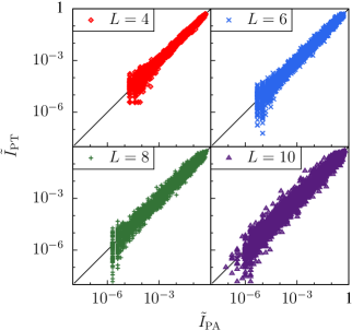
Figure 1: (Color online) Log-log (base $10$) scatter plots of $\tilde{I}_{\cal J}$. Each point represents a disorder realization. The horizontal position of the point is $\tilde{I}_{\cal J}$ measured in PA and the vertical position is the value of $\tilde{I}_{\cal J}$ measured in PT, for sizes, $L=4$, $6$, $8$ and $10$ at $T=0.2$.

Table 3: Comparison of the disorder averaged overlap weight near the origin, $I$ between PA and PT at $T=0.2$ for the same set of disorder realizations.

$L$	4	6	8	10
PA	0.0186(10)	0.0194(10)	0.0205(10)	0.0200(10)
PT	0.0185(9)	0.0196(9)	0.0205(10)	0.0198(10)

VI.2 Characteristic population sizes in PA and correlation times in PT

Next we consider quantities that are intrinsic to each algorithm and that are related to errors. Figure 2 is a logarithmic scatter plot of $\rho_{s}$, the entropic family size measured in PA, and $\tau^{q}_{\rm int}$, the integrated autocorrelation time for the spin overlap measured in PT. Each point represents a disorder realization; the horizontal position of the point is $\log_{10}\rho_{s}$ and the vertical position is $\log_{10}\tau^{q}_{\rm int}$. It is striking that the these two quantities are strongly correlated. Both $\rho_{s}$ and $\tau^{q}_{\rm int}$ are related to statistical errors in their respective algorithms and large values correspond to hard instances that require lots of computer resources to simulate accurately. It is clear that the hardness of an instance for PA and for PT is strongly correlated.

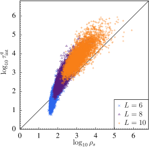
Figure 2: (Color online) Log-log scatter plot of $\rho_{s}$ (entropic family size for PA) vs $\tau_{\rm int}^{q}$ (integrated autocorrelation time of the spin overlap for PT). Each point represents a single disorder realization and there are roughly $5000$ disorder realizations each for sizes $L=6$, $8$, and $10$ at $T=0.2$.

Figure 3 shows histograms of $\log_{10}\rho_{s}$ (left panel) and $\log_{10}\tau^{q}_{\rm int}$ (right panel) for all $4945$ disorder realizations of size $L=10$ at $T=0.2$. Both distributions are very broad and both are skewed toward hard disorder realizations although the $\rho_{s}$ distribution is more sharply peaked than the $\tau^{q}_{\rm int}$ distribution.

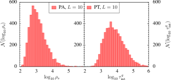
Figure 3: (Color online) Histogram of $\log_{10}\rho_{s}$ (left panel) and $\log_{10}\tau^{q}_{\rm int}$ (right panel) for all $4945$ disorder realizations, size $L=10$ at $T=0.2$.

Figure 4 is a log-linear plot of the disorder averages $[\log_{10}\rho_{s}]_{d}$ and $[\log_{10}\tau_{\rm int}]_{d}$ vs system size $L$. Square symbols (blue) are for PT at $T=0.2$, circular symbols (red) for PA at $T=0.2$, and triangular symbols (green) for PA at $T=0.42$. The nearly linear behavior suggests that both algorithms suffer exponential slowing with system size as expected. The fitted slope is greater for PT than for PA, however, one should be cautious in interpreting these fits as indicating better scaling for PA relative to PT. There is some upward curvature for PA in the data for both temperatures so the asymptotic scaling slope may be significantly larger than the finite-$L$ slope. In addition, $\tau_{\rm int}$ and $\rho_{s}$ are not strictly comparable quantities and, finally, neither algorithm has been carefully optimized. Nonetheless, one can safely conclude that PA is at least comparable in efficiency to PT for the sizes studied – system sizes that are of current scientific interest across applications.

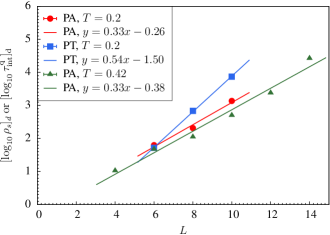
Figure 4: (Color online) Disorder averages $[\log_{10}\rho_{s}]_{d}$ for PA and $[\log_{10}\tau^{q}_{\rm int}]_{d}$ vs $L$. Square symbols (blue) are for PT at $T=0.2$, circular symbols (red) for PA at $T=0.2$, and triangular symbols (green) for PA at $T=0.42$. Straight lines are best linear fits to the data. Note that the behavior of $\rho_{t}$ is qualitatively similar to the behavior of $\rho_{s}$.

In Secs. IV.1 and IV.2, we introduced three characteristic population sizes, $\rho_{s}$, $\rho_{t}$, and $\rho_{f}$. Both $\rho_{s}$ [see Eq. (31)] and $\rho_{t}$ [see Eq. (28)] are obtained from the distribution of family sizes and are related to statistical errors while $\rho_{f}$ [see Eq. (20)] is obtained from the variance of the free-energy estimator and controls systematic errors. What is the relation between these three quantities for spin glasses? Figure 5 is a scatter plot of $\rho_{s}$ vs $\rho_{t}$ for system sizes $L=4$, $6$, $8$, and $10$. Each point represents a single disorder realization. It is clear that these two measures are strongly correlated with $\rho_{s}$ serving as a lower bound for $\rho_{t}$.

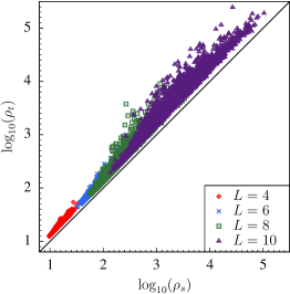
Figure 5: (Color online) Scatter plot of $\rho_{s}$, entropic family size vs $\rho_{t}$ the mean squared family size for sizes $L=4$, $6$, $8$, and $10$ at $T=0.2$.

Figure 6 is a scatter plot of $\rho_{s}$ vs $\rho_{f}$ for the $n=1000$ disorder realizations of size $L=14$ where each point represents a disorder realization. The value of $\rho_{f}$ is estimated for each disorder realization from $10$ runs with $R=3\times 10^{6}$ and $\rho_{f}$ is estimated as $R$ times the sample variance of $\beta{\tilde{F}}$ from the $10$ runs. Since it is obtained from only $10$ runs, $\rho_{f}$ has large statistical errors. The straight line is a best fit through the data points. It is clear that $\rho_{s}$ and $\rho_{f}$ are strongly correlated although $\rho_{f}$ is on average a factor of $1.6$ larger than $\rho_{s}$.

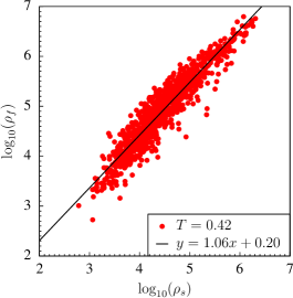
Figure 6: (Color online) Scatter plot of the entropic family size $\rho_{s}$ vs equilibration population size $\rho_{f}$ for $1000$ disorder realizations of size $L=14$ at $T=0.42$. The straight line is a best fit through the data.

The strong correlation between $\rho_{s}$ and $\rho_{f}$ justifies using $R>100\rho_{s}$ as an equilibration criterion. In principle, equilibration (systematic error) is controlled by $\rho_{f}$ but measuring $\rho_{f}$ requires multiple runs whereas measuring $\rho_{s}$ requires only a single run. Thus, except for situations where weighted averaging is used, it is more straightforward and reasonably well justified to require that the population size is some factor larger than $\rho_{s}$. Because $\rho_{t}$ is just as easy to measure as $\rho_{s}$, and $\rho_{t}>\rho_{s}$, and $\rho_{t}$ is more directly related to statistical errors, it may be preferable to use $\rho_{t}$ rather than $\rho_{s}$ as an equilibration criterion in future simulations.

VI.3 Convergence to equilibrium

Since statistical errors are much larger than systematic errors, in order to investigate systematic errors, i.e.,convergence to equilibrium, it is necessary to carry out a very large number of independent simulations of the same disorder realization. From these many runs, systematic errors can be studied as a function of population size $R$. In this section we examine in detail the convergence to equilibrium for two disorder realizations. One of these disorder realizations is the hardest $L=8$ sample as measured by $\rho_{s}$. This disorder instance was also studied in detail in Refs. Wang et al. (2015b) and Wang (2015a). We call this disorder realization “instance J8.” The second is an $L=4$ disorder realization that we call “instance J4.” Observables of the two instances are shown in Table 4.

Table 4: Equilibrium values of observables at $T=0.2$ for the two disorder instances studied in detail, J4 and J8, of sizes $L=4$ and $8$, respectively.

	$\rho_{f}$	$-\beta F$	$-E$	$\delta\tilde{E}/\beta\delta{\tilde{F}}$	$I$	$\delta\tilde{I}/\beta\delta{\tilde{F}}$
J4	$33$	$584.138$	$116.541$	$0.0542$	$0.0929$	$0.0843$
J8	$9.0\times 10^{3}$	$4457.53$	$890.186$	$0.0355$	$0.00104$	$0.00105$

We first carefully examine, for instance J8, the convergence to equilibrium as a function of $R$ for the energy estimator $\tilde{E}$ and the dimensionless free-energy estimator $\beta{\tilde{F}}$ at temperature $T_{0}=0.2$. Figure 7 shows histograms of the deviation of the dimensionless free-energy estimator from its equilibrium value, $\Delta\beta\tilde{F}$ (top row), the deviation of the energy estimator from its equilibrium value, $\Delta\tilde{E}$ (middle row), and a scatter plot of their joint distribution (bottom row) for population sizes, $R=10^{3}$, $10^{4}$, $10^{5}$ and $10^{6}$ (from left to right, respectively). For each population size we carried out ${\cal M}=1000$ independent simulations of J8. The ‘exact’ equilibrium values, listed in Table 4, are obtained from a weighted average of the $1000$ runs at the largest population size, $R=10^{6}$. For the two smaller populations the distributions are highly non-Gaussian but as $R$ increases the joint distribution approaches a bivariate Gaussian distribution. The joint distribution initially consists of two well-separated peaks representing the fact for small $R$ most or all of the population is frequently stuck in a metastable state with both a higher free energy and higher energy. This bimodal distribution is a feature of this particular disorder realization and explains, in part, the computational hardness of this sample. Since $\rho_{f}\approx 10^{4}$, the $R=10^{3}$ populations are not equilibrated and the $R=10^{4}$ populations are barely equilibrated. Finally, for $R=10^{6}$, the populations are reasonably well equilibrated so that the $\tilde{E}$ and $\beta\tilde{F}$ distributions are close to Gaussian and the joint distribution is close to a bivariate Gaussian. The slope of the regression line through the scatter plot representing the $R=10^{6}$ joint distribution is an estimator of the quantity $\delta\tilde{E}/\beta\delta{\tilde{F}}$, which controls the error in the energy estimator, see Eq. (22).

We can assess more quantitatively whether $\beta{\tilde{F}}$ and $\tilde{E}$ are described by a bivariate normal distribution. From the ${\cal M}=1000$ runs, we measured the skewness and kurtosis of both variables. For instance, for J8 and $R=10^{6}$, the skewness and (excess) kurtosis of the dimensionless free-energy runs is $0.047$ and $0.043$, respectively. Both values are statistically indistinguishable from values that would be obtained from a sample of $1000$ normal random variates. The corresponding values of skewness and kurtosis for the energy are $0.121$ and $0.152$, respectively. Although larger, both values are consistent with a sample of $1000$ normal random variates. The joint distribution is, however, only marginally consistent with a bivariate Gaussian, as measured by the Mardia Mardia (1970) combined skewness and kurtosis test ($p=0.06$). For instance, for J8 at $R=10^{6}$, $R/\rho_{f}\approx 10^{2}$. For J4 at population size $R=10^{6}$ we have $R/\rho_{f}\approx 3\times 10^{4}$ and from ${\cal M}=5000$ runs the joint distribution cannot be distinguished from a bivariate Gaussian by the Mardia combined test ($p=0.4$).

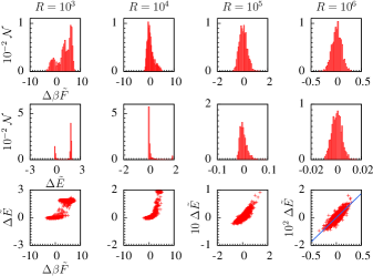
Figure 7: (Color online) Histograms of $\Delta\beta{\tilde{F}}$ (top row), histograms of $\Delta\tilde{E}$ (middle row), and scatter plots representing the joint distributions of $\Delta\tilde{E}$ and $\Delta\beta{\tilde{F}}$ for instance J8 at $T=0.2$ (bottom row). Each column represents a given population size and, from left to right, $R=10^{3}$, $10^{4}$, $10^{5}$, and $10^{6}$, respectively. The slope of the regression line in the $\Delta\tilde{E}$ vs $\Delta\beta{\tilde{F}}$ scatter plot for $R=10^{6}$ (lower right box) is the estimator of $\delta\tilde{E}/\beta\delta{\tilde{F}}$.

Next, we study the convergence of the mean values of observables to their equilibrium values as a function of $R$. For each observable ${\cal A}$ we obtain the mean value for a single run $\langle\tilde{\cal A}\rangle$ from a simple average over all ${\cal M}$ runs for each population size and we obtain the equilibrium value from a weighted average over all runs at the largest size. Figure 8 shows $\langle\Delta\beta{\tilde{F}}\rangle$, $\langle\Delta\tilde{E}\rangle$, and $\langle\Delta\tilde{I}\rangle$, the deviation of the estimators of the dimensionless free energy, energy and overlap near the origin from their respective equilibrium values, as a function of population size $R$ for instance J4. The straight lines are theoretical curves from Eqs. (22) and (23) using the values of $\rho_{f}$ and $\delta\tilde{\cal A}/\beta\delta{\tilde{F}}$ estimated at $R=10^{6}$ and given in Tab. 4. We see that there is reasonable quantitative agreement with the predicted $1/R$ dependence of the systematic errors. The $R=10^{6}$ data point is not shown because statistical errors in measuring the exact values $\langle{\cal A}\rangle$ are comparable here to systematic errors in $\langle\tilde{\cal A}\rangle$. Probing the $1/R$ regime of systematic errors proved quite difficult because of the much larger statistical errors. For example, to sufficiently reduce statistical errors for instance J4 we used ${\cal M}=32\,000$ independent runs to obtain the $R=10^{5}$ averages $\langle\tilde{\cal A}\rangle$ in Fig. 8 and $M=5000$ independent runs at $R_{0}=10^{6}$ to obtain “exact” equilibrium values $\langle{\cal A}\rangle$ from weighted averaging.

Figure 9 shows similar results for the size $8$ instance J8. Since the joint distributions are far from bivariate Gaussians for the smaller values of $R$ for instance J8, the theoretical predictions for $\langle\Delta\tilde{E}\rangle$, and $\langle\Delta\tilde{I}\rangle$ are poor for the smaller population sizes. The points for $R=10^{6}$ in Fig. 9 are in essentially perfect agreement with the theoretical predictions of Eq. (22), however, since $\rho_{f}$ and $\delta\tilde{\cal A}/\beta\delta{\tilde{F}}$ are all measured at $R=10^{6}$ this agreement is really just a check that the joint distribution is close to the assumed bi-variate Gaussian form.

Figure 8: (Color online) Log-log plot showing the deviations from equilibrium (systematic errors) in the dimensionless free energy, $\langle\Delta\beta{\tilde{F}}\rangle$ (red circles), energy, $\langle\Delta\tilde{E}\rangle$ (blue squares) and overlap near the origin $\langle\Delta\tilde{I}\rangle$ (green triangles) as a function of population size $R$ for instance J4 at $T=0.2$. The straight lines are theoretical curves based on Eqs. (22) and (23).

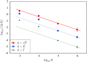
Figure 9: (Color online) Log-log plot showing the deviations from equilibrium (systematic errors) in the dimensionless free energy $\langle\Delta\beta{\tilde{F}}\rangle$ (red circles), energy, $\langle\Delta\tilde{E}\rangle$ (blue squares), and overlap near the origin $\langle\Delta\tilde{I}\rangle$ (green triangles) as a function of population size $R$ for instance J8 at $T=0.2$. The straight lines are theoretical curves based on Eqs. (22) and (23).

Next, we examine the convergence of the various characteristic population sizes to their asymptotic values. Figure 10 shows the finite size estimators of $\rho_{f}$, $\rho_{s}$, and $\rho_{t}$ versus the population size $R$ at which they are measured for instance J8. For this instance all of these quantities have values near $10^{4}$ and their values are near their asymptotic values for the two largest population sizes for which $R\geq 10\rho$. The rapid convergence of $\rho_{f}$ supports the hypothesis that equilibrium is approached as $1/R$. We do not show a similar graph for instance J4 because all three $\rho$ measures are already saturated to their asymptotic values within statistical errors even for smallest population sizes studied.

Figure 10: (Color online) Log-log plot showing estimators of the equilibration sizes $\rho_{f}$ (red circles), $\rho_{t}$ (blue squares), and $\rho_{s}$ (green triangles) as a function of population size $R$ at $T=0.2$ for instance J8.

Finally, we can also gain some insights into weighted averaging from the detailed study of a single instance. The question we address is whether a single run is significantly better than a weighted average with the same total population size. We computed the systematic error in the weighted average of the dimensionless free energy $\beta{\tilde{F}}$ of instance J8 for $R_{0}=10^{3}$ and $M=10$ and compared it to the systematic error for a single run with $R=MR_{0}=10^{4}$. We used ${\cal M}=1000$ independent runs with $R=10^{3}$ to compute the mean $\langle\beta\overline{F}\rangle$ and standard error of the weighted average. To compute the mean, we take $M=10$ random values from the set of ${\cal M}=1000$ runs, compute the weighted average, and then take the mean of that weighted average over many such experiments. We used the blocking method to compute the standard error of the mean. We used ${\cal M}=1000$ runs with $R=10^{4}$ to obtain $\langle\beta{\tilde{F}}\rangle$ and its error. We found that $\langle\Delta\beta\overline{F}\rangle=0.75\pm 0.12$, while $\langle\Delta\beta{\tilde{F}}\rangle=0.63\pm 0.04$. Thus, the weighted average has roughly the same systematic errors as the single long run. Note that in this example, $R_{0}<\rho_{f}$. We expect the differences between weighted averaging and a single long run to vanish as $R_{0}/\rho_{f}\rightarrow\infty$. Unfortunately, even with $1000$ independent runs, we did not achieve sufficient statistical power to distinguish the weighted average clearly from a single long run although we expect the former to have somewhat larger systematic errors. These considerations lead to the following conjecture: Suppose one has available a fixed total amount of work defined by a total population size, $R_{0}M$ such that $R_{0}\gtrsim\rho_{f}$, then the weighted average obtained from $M$ runs each with population size $R_{0}$ is statistically indistinguishable from a single long run with population $R=R_{0}M$. However, the discussion in Sec. IV.3 comparing PA and PT for disorder averaging is relevant here as well. If a sufficiently large disorder sample is simulated, the differences in systematic errors between a weighted average and a single long run could become relevant. While additional work to understand the systematic errors in weighted averaging is needed, it seems clear that weighted averaging is a useful tool for studying hard problems requiring very large total populations.

VII Discussion

We have shown that population annealing is an effective and efficient algorithm for simulating spin glasses. It is comparably efficient to parallel tempering, the standard in the field, and it has several advantages.

The first advantage is that it is naturally a massively parallel algorithm. The convergence to equilibrium occurs as the population size grows and each replica in the population can be simulated independently. Since realistic spin-glass simulations using population annealing require population sizes of the order of $10^{6}$ or more, there is a much greater scope for parallelism than in parallel tempering where in spin-glass simulations typically less than $100$ replicas are simulated in parallel. To put this difference in perspective, recall that parallel tempering is a Markov-chain Monte Carlo algorithm while population annealing is a sequential Monte Carlo algorithm. From a computational complexity perspective, when going from a Markov-chain Monte Carlo algorithm to a sequential Monte Carlo algorithm, time is exchanged for hardware so that long running times can be exchanged for massive parallelism. The downside of exchanging time for hardware is that population annealing has much larger memory requirements than parallel tempering.

A second advantage of population annealing is access to weighted averaging, which allows multiple independent runs of PA to be combined to improve both statistical and systematic errors. Weighted averaging opens the door to distributed computing. It is potentially possible to quickly simulate very difficult to equilibrate instances of spin glasses or other hard statistical-mechanical models by distributing the work over a large and inhomogeneous set of computational resources. The only information that needs to be collected and analyzed centrally from each run is the estimators of observables together with the estimator of the free energy.

Apart from its large memory usage, the main disadvantage of population annealing (and sequential Monte Carlo methods in general) is that it converges to equilibrium inversely in population size whereas parallel tempering (and Markov-chain Monte Carlo methods in general) converges exponentially. In most situations, this difference is moot because statistical errors are much larger than systematic errors. However, for very high precision disorder averages, it is possible that the exponential convergence of parallel tempering would be an advantage over the power law convergence of population annealing.

Thus far, the implementations of population annealing for large-scale simulations have used a simple annealing schedule. The temperature set is uniform in the inverse temperature and there are a constant number of Metropolis sweeps at each temperature. It is plausible that a more complicated annealing schedule might be more efficient. It is perhaps possible that the annealing schedule can be adaptively adjusted to the particular problem instance in analogy to related proposals for parallel tempering simulations Katzgraber et al. (2006a); Bittner et al. (2008). It might also improve efficiency to change the population size with temperature. In addition, our implementation uses the Metropolis algorithm at every temperature, however, at low temperatures kinetic Monte Carlo might be preferable and, at intermediate temperatures cluster moves, might be useful Zhu et al. (2015).

Population annealing is a general method suitable for simulating equilibrium states of systems with rough free-energy landscapes. It can be applied to any system for which there is a parameter, such as temperature, that takes the equilibrium distribution from an easy to simulate region, e.g., at high temperature, to a hard to simulate region, e.g., at low temperature. In addition to spin systems, population annealing may prove useful in simulating the equilibrium states of dense fluids or complex biomolecules.