Complexity of anticipated rejection algorithms
and the Darling–Mandelbrot distribution

Abstract

We study in limit law the complexity of some anticipated rejection random sampling algorithms. We express this complexity in terms of a probabilistic process, the threshold sum process. We show that, under the right conditions, the complexity is linear and admits as a limit law a so-called Darling–Mandelbrot distribution, studied by Darling (1952) and Lew (1994). We also give an explicit form to the density of the Darling–Mandelbrot distribution and derive some of its analytic properties.

1 Introduction

This paper aims at answering the following algorithmic question: consider a program $P$ that performs a random number of elementary operations and then terminates. Our goal is to have $P$ performing $n$ operations in one run. To do that, we run the program $P$ until it reaches $n$ operations; if it terminates before that, we simply restart it. The question is, how many elementary operations must we perform to reach this goal?

Algorithms of this type are abundant in the field of random sampling, where they are known as anticipated rejection algorithms. Given a class of discrete objects, a random sampling algorithm takes an integer $n$ as input and outputs a random object of size $n$ according to a specific (usually uniform) distribution. Given a random sampling algorithm for a class $\mathcal{A}$ and a subclass $\mathcal{B}$ of $\mathcal{A}$, an element of $\mathcal{B}$ can be sampled using a rejection algorithm: we repeatedly sample elements of $\mathcal{A}$ until we find one in $\mathcal{B}$. This algorithm can be improved when it is possible to know in advance, during the sampling procedure, that the drawn element is not going to be in $\mathcal{B}$: we can then prematurely reject the sample and start over, saving computing time. This scheme is called anticipated rejection. Assuming that sampling an element of $\mathcal{A}$ costs $n$ elementary operations, this fits into the framework outlined above.

Such algorithms are found for example in Barcucci et al. (1994, 1995), sampling prefixes of Motzkin paths (the so-called Florentine algorithm). Somewhat miraculously, this algorithm achieves an average linear time complexity, as, on average, the number of necessary trials is $\mathcal{O}(\sqrt{n})$ and each trial costs $\mathcal{O}(\sqrt{n})$. We show that this phenomenon is not isolated, but rather happens in a wider range of cases. Other algorithms of this family exist, sampling Schröder prefixes Penaud et al. (2001), unary-binary trees Bacher et al. (2014) and constrained random walks.

In this paper, we study the full limit distribution of the complexity of these algorithms. This problem leads us to define a probabilistic process, the threshold sum process. Our main result is that, if the base distribution has a tail with exponent $\alpha$ in a certain range, this process admits a limit distribution depending only on $\alpha$. This universality phenomenon is reminiscent of Lévy’s well-known theory of $\alpha$-stable distributions, which also deals with sums of independent random variables Gnedenko and Kolmogorov (1968).

Surprisingly, our limiting distribution has already been studied in relation to a different problem, namely, the ratio between the sum and the maximum of a fixed number of i.i.d. random variables. It was first studied by Darling Darling (1952), then apparently by Mandelbrot in unpublished work, and by Lew Lew (1994), who named it the Darling–Mandelbrot distribution. This distribution has a parameter $\alpha$, with $0<\alpha<1$; it is supported on $\mathbb{R}_{+}$ and is defined by its characteristic function:

$$\phi_{\alpha}(s)=\frac{(-is)^{-\alpha}}{-\alpha\gamma(-\alpha,-is)}=\Biggl{(}1-\sum_{n=1}^{\infty}\frac{\alpha}{n-\alpha}\frac{(is)^{n}}{n!}\Biggr{)}^{-1}\text{,}$$ (1)

where in the first expression, $\gamma(\cdot,\cdot)$ denotes the lower incomplete gamma function. The second expression allows to easily extract the moments of the distribution as rational functions of $\alpha$. Lew showed that the distribution has an exponential tail; moreover, we show that its density is non-analytic at all integer points. Both properties contrast with the Lévy distributions, which have an analytic density and a heavy tail.

In the case of the Florentine algorithm (which corresponds to an exponent $\alpha=1/2$, as seen below), an expression of the Laplace transform of the limit distribution already appears in Louchard (1999), namely:

$$\frac{1}{e^{-z}+\sqrt{\pi z}\operatorname{erf}(\sqrt{z})}\text{.}$$

We readily check that this expression is equivalent to $\phi_{1/2}(iz)$, the Laplace transform of the Darling-Mandelbrot distribution of parameter $1/2$.

The paper is organized as follows. In Section 2, we define the threshold sum process and show that, under some conditions, its limit distribution is a Darling–Mandelbrot distribution. In Section 3, we give an explicit form for the Darling–Mandelbrot density and give analytic results expanding those of Lew. Finally, in Section 4, we use these results to analyse some anticipated rejection algorithms.

2 The threshold sum process

In the following, let $(X_{i})_{i\geq 0}$ be a sequence of independent and identically distributed random variables with values in $\mathbb{N}$ or $\mathbb{R}_{+}$ and unbounded support. We denote by $F(x)$ the complementary cumulative distribution function of the $X_{i}$’s:

$$F(x)=\mathbb{P}(X_{i}\geq x)\text{.}$$

Let $t\geq 0$ and let $I(t)$ be the smallest index such that $X_{I(t)}\geq t$. Define the threshold sum process (TSP) $Y_{t}$ as:

$$Y_{t}=X_{0}+\dotsb+X_{I(t)-1}\text{.}$$

The number $t$ is called the threshold. This process resembles the classical sum of independent random variables, but the number of summands $I(t)$ is here a random variable depending on the real parameter $t$. Our main result on this process is the following.

Theorem 2.1

Assume that, as $x$ tends to infinity, $F(x)$ is equivalent to $c\,x^{-\alpha}$ for some $c>0$ and $\alpha>0$. Then, as $t$ tends to infinity, the random variable $Y_{t}$ satisfies:

• if $\alpha<1$, then $Y_{t}/t$ converges in distribution to the Darling–Mandelbrot law of parameter $\alpha$;

• if $\alpha=1$, then $Y_{t}/(t\log t)$ converges in distribution to the exponential law;

• if $\alpha>1$, then $Y_{t}/(t^{\alpha}c^{-1}\mu)$, where $\mu=\mathbb{E}(X_{i})$, converges in distribution to the exponential law.

To us, the most interesting case is $\alpha<1$, where the behavior of $Y_{t}$ is strongly universal in that it only depends on the exponent $\alpha$. Moreover, the scaling factor is always $t$ in that range (this is different from Lévy’s theory of sums of i.i.d. random variables, where the scaling factor is a power of $t$ depending on $\alpha$). For $\alpha=1$, the scaling factor is augmented by a $\log t$ factor; for $\alpha>1$, the scaling factor is higher and we have a lesser form of universality, with the limit scaled by $\mu/c$. Consequences of these facts to the analysis of algorithms are discussed in Section 4.

Proof

We prove this result using Lévy’s Continuity Theorem, which states that a sequence of random variables tends in distribution to some limit if their characteristic functions converge pointwise to the characteristic function of the limit distribution.

Let $\psi_{t}(s)=\mathbb{E}(e^{isY_{t}/\tau})$ be the characteristic function of the random variable $Y_{t}/\tau$, where $\tau$ is a scaling factor (depending on $t$) to be specified later on. The index $I(t)$ is geometrically distributed with parameter $F(t)$, which is the probability that $X_{i}\geq t$. The random variables $X_{0},\dotsc,X_{I(t)-1}$ are constrained to be less than $t$; let $\chi_{t}(s)=\mathbb{E}(e^{isX/t}|X<t)$ be the characteristic function of such a constrained variable. We have:

$$\psi_{t}(s)=\frac{F(t)}{1-\bigl{(}1-F(t)\bigr{)}\chi_{t}(s/\tau)}\text{.}$$

On the other hand, we have:

$$\chi_{t}(s)=\frac{1}{1-F(t)}\sum_{n=0}^{\infty}M_{t,n}\frac{(is)^{n}}{n!}\text{,}\qquad\text{with}\qquad M_{t,n}=\int_{0}^{t}x^{n}dF(x)\text{.}$$

We therefore have:

$$\psi_{t}(s)=\frac{F(t)}{\displaystyle 1-\sum_{n=0}^{\infty}\frac{M_{t,n}}{\tau^{n}}\frac{(is)^{n}}{n!}}=\frac{1}{\displaystyle 1-\sum_{n=1}^{\infty}\frac{M_{t,n}}{\tau^{n}F(t)}\frac{(is)^{n}}{n!}}\text{,}$$

where the last simplification follows from the fact that $M_{t,0}=1-F(t)$.

Consider first the case where $\alpha<1$. Using integration by parts, we find that the term $M_{t,n}$ satisfies as $t$ tends to infinity:

$$M_{t,n}=-t^{n}F(t)+\int_{0}^{t}nx^{n-1}F(x)dx\sim\frac{\alpha}{n-\alpha}\,c\,t^{n-\alpha}.$$

Moreover, as $F$ is nonincreasing, we have a bound $F(x)\leq c^{\prime}x^{-\alpha}$ for some constant $c^{\prime}$. This enables us to dominate $M_{t,n}$ by:

$$M_{t,n}\leq\frac{n}{n-\alpha}c^{\prime}t^{n-\alpha}.$$

Picking $\tau=t$, a dominated convergence argument and the expression (1) therefore show that the characteristic function $\psi_{t}(s)$ tends to the characteristic function $\phi_{\alpha}(s)$ of the Darling–Mandelbrot distribution. We conclude using Lévy’s theorem.

If $\alpha=1$, we have $M_{t,1}\sim c\log t$ as $t$ tends to infinity; if $\alpha>1$, $M_{t,1}$ tends to the finite value $\mu$. This means that the ratio $M_{t,1}/[\tau F(t)]$ tends to $1$ with the respective values $\tau=t\log t$ and $\tau=t^{\alpha}\mu/c$. Moreover, in both cases, all the higher moments satisfy $M_{t,n}=\mathcal{O}(t^{n-1})$ and are therefore negligible before $\tau^{n}F(t)$. This means that $\psi_{t}(s)$ satisfies:

$$\psi_{t}(s)\to\frac{1}{1-is}\text{,}$$

which is the characteristic function of the exponential distribution.

3 The Darling–Mandelbrot density

This section is devoted to the computation and the derivation of properties of the density, denoted by $g$, of the Darling–Mandelbrot distribution. By studying the Laplace transform, Lew Lew (1994) determined that $g$ is a continuous function satisfying:

$$g(x) =C_{0}x^{\alpha-1}+\mathcal{O}(1)\text{,} \qquad x \to 0^{+}\text{;}$$ (2)

$$g(x) =\frac{a_{0}}{\alpha}e^{-a_{0}(1+x)}+\mathcal{O}(e^{-a_{1}x})\text{,} \qquad x \to\infty\text{,}$$ (3)

where $C_{0}$ is the constant:

$$C_{0}=\frac{\sin(\alpha\pi)}{\pi}=\frac{1}{\Gamma(1-\alpha)\Gamma(\alpha)}$$ (4)

and where $-a_{0}$ is the real zero of the function $z\mapsto z^{\alpha}\gamma(-\alpha,z)$ and $a_{1}>a_{0}$ (see the reference for details).

3.1 Explicit forms of the density

Theorem 3.1

Let $0<\alpha<1$. The Darling–Mandelbrot density $g(x)$ is equal to:

$$g(x)=\sum_{k=0}^{\infty}g_{k}(x)\text{,}$$ (5)

where the function $g_{k}(x)$ is continuous for $x>0$, supported for $x>k$, analytic on its support, and has the two following equivalent definitions.

• Let $a(x)$ and $b(x)$ be the functions, supported for $x>0$ and $x>1$ respectively, defined by:

  $$a(x)=C_{0}x^{\alpha-1}\qquad\text{and}\qquad b(x)=-C_{0}\frac{(x-1)^{\alpha}}{x}\text{,}$$ (6)

  where $C_{0}$ is defined by (4). Then $g_{k}(x)$ is equal to the convolution product:

  $$g_{k}(x)=a*\underbrace{b*\dotsm*b}_{\text{$k$ times}}\,(x)\text{.}$$ (7)

• Let:

  $$\beta_{k}=\alpha+k(1+\alpha)\qquad\text{and}\qquad C_{k}=\frac{1}{\Gamma(1-\alpha)\Gamma(-\alpha)^{k}\Gamma(\beta_{k})}\text{.}$$ (8)

  Then $g_{k}(x)$ has the power series representation convergent for $k<x<k+1$ and analytically continuable for $x\geq k+1$:

  $$g_{k}(x)=C_{k}(x-k)^{\beta_{k}-1}\sum_{n_{1},\dotsc,n_{k}\geq 0}\frac{(1{+}\alpha)_{n_{1}}\dotsm(1{+}\alpha)_{n_{k}}}{(\beta_{k})_{n_{1}+\dotsb+n_{k}}}(k-x)^{n_{1}+\dotsb+n_{k}}\text{,}$$ (9)

  where $(y)_{n}=\Gamma(y+n)/\Gamma(y)$ is the Pochhammer symbol for the rising factorial.

Again, we make some remarks before proving the theorem. First, since the summand $g_{k}(x)$ has support for $x>k$, the infinite sum in (5) is locally finite, which justifies its existence and shows that $g$ is continuous. Moreover, since $b(x)$ is negative, the summands alternate in sign. In particular, if $x\leq 1$, we have $g(x)=g_{0}(x)=C_{0}x^{\alpha-1}$. This shows that the error term in (2) is in fact zero in that range. In the case $k=1$, the sum in (9) takes the form of a hypergeometric function:

$$g_{1}(x)=C_{1}(x-1)^{2\alpha}\,{}_{2}F_{1}(1,1+\alpha;1+2\alpha;1-x)\text{.}$$

For $\alpha=1/2$, this simplifies into:

$$g_{1}(x)=\frac{x^{-1/2}-1}{\pi}\text{.}$$

The theorem also enables us to find the singularities of the density $g(x)$. Since the leading term in the sum in (9) is $1$, the function $g_{k}(x)$ has a singularity at $k$ of the form:

$$g_{k}(x)=C_{k}(x-k)^{\beta_{k}-1}\,\mathbf{1}_{x>k}+\mathcal{O}\bigl{(}(x-k)^{\beta_{k}}\bigr{)}\text{.}$$

Moreover, as the function $g_{k}(x)$ is analytic for $x>k$ and the sum (5) is locally finite, the density $g(x)$ is singular at all integer points and analytic otherwise, the singularity at the point $x=k$ being contributed by $g_{k}(x)$.

Finally, we note that although the sum in (5) behaves very well locally (indeed, it’s locally finite), it’s not the case globally: as $x$ tends to infinity, $g_{k}(x)$ behaves like $x^{k\alpha-1}$ and so alternately tends to $\pm\infty$ for $k$ sufficiently large. Yet, as found by studying the Laplace transform, the sum converges exponentially fast to zero.

In order to plot the density $g(x)$, the most adequate characterisation is (7), or better yet, the differential equation of the forthcoming Theorem 3.2, which was used to produce Figure 1.

Figure 1: Plots of the density $g(x)$ for $\alpha=1/4$, $\alpha=1/2$ and $\alpha=3/4$ (from left to right). Dashed, the continuation of the partial sums $g_{0}+\cdots+g_{k}$ beyond $x=k+1$. The precision is far beyond line thickness (as easily obtained through the characterisation of Theorem 3.2).

Proof (of Theorem 3.1)

Let us first prove the convolution product representation. From the identity (1) we find the Laplace transform of $g(x)$, that we denote by $G(z)$:

$$G(z)=\phi_{\alpha}(iz)=\frac{z^{-\alpha}}{-\alpha\gamma(-\alpha,z)}\text{.}$$

We transform this into:

$$G(z)=\frac{z^{-\alpha}}{-\alpha\bigl{(}\Gamma(-\alpha)-\Gamma(-\alpha,z)\bigr{)}}=\sum_{k\geq 0}A(z)B(z)^{k}\text{,}$$

where $\Gamma(\cdot,\cdot)$ is the upper incomplete gamma function and:

$$A(z)=\frac{z^{-\alpha}}{\Gamma(1-\alpha)}\qquad\text{and}\qquad B(z)=\frac{\Gamma(-\alpha,z)}{\Gamma(-\alpha)}$$

(if $z$ is large enough so that $\lvert B(z)\rvert<1$; numerically, $\mathfrak{Re}(z)>0.107878\ldots$ suffices, uniformly for all $\alpha$).

Noting that $\Gamma(1-\alpha)\Gamma(\alpha)=-\Gamma(-\alpha)\Gamma(1+\alpha)$, the following elementary computations show that the functions $a(x)$ and $b(x)$ defined in (6) have Laplace transforms $A(z)$ and $B(z)$, respectively:

$$\int_{0}^{\infty}x^{\alpha-1}e^{-xz}dx =z^{-\alpha}\int_{0}^{\infty}x^{\alpha-1}e^{-x}dx$$

$$=z^{-\alpha}\Gamma(\alpha)\text{;}$$

$$\int_{1}^{\infty}\frac{(x-1)^{\alpha}}{x}e^{-xz}dx =\int_{z}^{\infty}\int_{1}^{\infty}(x-1)^{\alpha}e^{-xy}dxdy$$

$$=\int_{z}^{\infty}y^{-1-\alpha}\Gamma(1+\alpha)e^{-y}dy$$

$$=\Gamma(-\alpha,z)\Gamma(1+\alpha)\text{.}$$

Inverse Laplace transform thus yields (7). The function $g_{k}(x)$ is analytic for $x>k$ as the convolution product of analytic functions.

Let us now prove the power series representation. Let $1<x<2$. A Taylor expansion of the function $b(x)$ yields:

$$b(x)=\frac{1}{\Gamma(-\alpha)}\sum_{n\geq 0}(-1)^{n}\frac{(x-1)^{\alpha+n}}{\Gamma(1+\alpha)}.$$

The identity (9) then follows from (7) using the classic formula:

$$f_{r_{1}}^{(\alpha_{1})}*\dotsm*f_{r_{k}}^{(\alpha_{k})}=f_{r_{1}+\dotsb+r_{k}}^{(\alpha_{1}+\dotsb+\alpha_{k})}\text{,}\qquad f_{r}^{(\alpha)}(x)=\frac{(x-r)^{\alpha-1}}{\Gamma(\alpha)}\mathbf{1}_{x>r}\text{.}$$ (10)

Finally, since $g_{k}(x)$ is analytic for $x>k$, its value for $x\geq k+1$ is found by analytic continuation.

3.2 Differential equations satisfied by the density

In this section, we characterize the density $g$ not explicitly, but implicitly as the solution of differential equations. Since $g$ is singular at all integer points, all differential equations are understood to be satisfied only outside singular points.

Theorem 3.2

The density $g(x)$ is the only continuous solution of the non-linear differential equation:

$$xg^{\prime}(x)+(1-\alpha)g(x)=-\alpha\,g*g(x-1)\text{,}$$ (11)

with initial condition (2).

As the density $g$ is positive, this result shows in particular that $g$ is decreasing. In fact, the equation above can be rewritten as

$$\frac{\mathrm{d}}{\mathrm{d}x}\big{(}x^{1-\alpha}g(x)\big{)}=-\alpha x^{\alpha}g*g(x-1)\text{.}$$

This makes evident the stronger statement that $x^{1-\alpha}g(x)$ is nonincreasing. This answers a question of Lew, who suggested that $g(x)$ might show oscillations for small values of $\alpha$.

Proof

Let us prove that $g$ satisfies the equation. One way to proceed is to differentiate the Laplace transform $G(z)$. One can also directly use the representations of Theorem 3.1. Another way, that we detail here, is to compare the threshold sum processes at thresholds $t$ and $u$, with $u\geq t$. We have:

$$Y_{u}=\begin{cases}Y_{t}&\text{if $X_{I(t)}\geq u$;}\\ Y_{t}+X_{I(t)}+Y^{\prime}_{u}&\text{if $t\leq X_{I(t)}<u$,}\end{cases}$$

where $Y^{\prime}_{u}$ is independent from $Y_{t}$ and distributed like $Y_{u}$.

Now, set $u=\lambda t$ and let $t$ tend to infinity. The event $X_{I(t)}\geq u$ occurs with probability $F(u)/F(t)\to\lambda^{-\alpha}$. If it does not, we have $X_{I(t)}=t+\mathcal{O}(\lambda-1)$. Dividing by $t$ and recalling that $Y_{t}/t$ tends to the law of density $g$, we get:

$$\lambda^{-1}g(\lambda^{-1}x)=\lambda^{-\alpha}g(x)+(1-\lambda^{-\alpha})\bigl{(}g*g(x-1)+\mathcal{O}(\lambda-1)\bigr{)}\text{.}$$

We recover (11) at first order in $\lambda-1$.

To show the uniqueness of the solution, we note that the right hand side of (11) depends only on the values of $g(y)$ for $y<x-1$; in particular, it is zero for $x<1$. This enables us to solve iteratively the equation on the intervals $[k,k+1]$, treating the equation as an inhomogenous linear differential equation, with the initial value $f(k)$ found by continuity. This determines the solution uniquely.

Our final result writes the density $g$ as the solution of linear differential equations. Write $d_{x}=\mathrm{d}/\mathrm{d}x$ and let $D_{k}$ and $E_{k}$ be the differential operators:

$$D_{k}=d_{x}(x-k)-(k+1)\alpha\text{;}\qquad\qquad E_{k}=D_{k-1}\dotsm D_{0}\text{.}$$

Theorem 3.3

The operator $E_{k}$ cancels the functions $g_{0},\dotsc,g_{k-1}$ defined in Theorem 3.1. In particular, it cancels the density $g$ on the interval $[0,k]$.

Proof

To prove the theorem, we need the following elementary facts about convolution products:

$$x(u*v)=(xu)*v+u*(xv)\text{;}\qquad\qquad(u*v)^{\prime}=u^{\prime}*v\text{.}$$

We first prove by induction that, for $0\leq\ell\leq k$, we have:

$$E_{\ell}\cdot g_{k}=\frac{k!}{(k-\ell)!}a_{\ell}*b^{*k-\ell}\text{,}$$

where

$$a_{\ell}(x)=\frac{(x-\ell)^{(\ell+1)\alpha-1}}{\Gamma(1-\alpha)\Gamma(-\alpha)^{\ell}\Gamma\bigl{(}(\ell+1)\alpha\bigr{)}}\mathbf{1}_{x>\ell}\text{.}$$

For $\ell=0$, this is obvious as $a_{0}=a$. Otherwise, assume that the identity is true at rank $\ell$ and apply the operator $D_{\ell}$ to it. Using the above properties of convolution products, we have:

$$E_{\ell+1}\cdot g_{k}=\frac{k!}{(k-\ell)!}(D_{\ell}\cdot a_{\ell})*b^{*k-\ell}+\frac{k!}{(k-\ell-1)!}a_{\ell}*(xb)^{\prime}*b^{*k-\ell-1}\text{.}$$

Since $D_{\ell}$ annihilates $a_{\ell}$, we conclude using the fact that $a_{\ell}*(xb)^{\prime}=a_{\ell+1}$ found using formula (10).

At $\ell=k$, we thus find $E_{k}\cdot g_{k}=k!\,a_{k}$. Since $D_{k}\cdot a_{k}=0$, we have indeed $E_{\ell}\cdot g_{k}=0$ for $\ell>k$.

4 Applications

In this section, we apply our results to the analysis in limit law of random sampling algorithms. In all cases, this complexity is linked to a threshold sum process that falls within the conditions of Theorem 2.1. Among the three regimes in this theorem, the most favorable is the first one, with the scaling factor $t$ meaning that the algorithm has linear complexity.

In the following, we consider an anticipated rejection algorithm based on a process with survival probability at time $t$ asymptotic to $c\,t^{-\alpha}$; the algorithm consists in running the process repeatedly until it reaches time $t$. Since the successful run takes time $t$, the complexity normalized by $t$ follows a Darling-Mandelbrot distribution shifted by one, with characteristic function $e^{is}\phi_{\alpha}(s)$ (this coincides with Darling’s initial definition). We denote by $\mathcal{D}(\alpha)$ this shifted distribution.

In some cases, the algorithm has a second round of rejection on top of anticipated rejection, i.e., it may fail and be restarted upon reaching the target $t$. Let us assume that it succeeds with a fixed probability $p$. The overall complexity of the algorithm is then of the form $Y_{1}+\dotsb+Y_{Z}$, where the $Y_{i}$’s are independent variables following the law $\mathcal{D}(\alpha)$ and $Z\geq 1$ is geometrically distributed with parameter $p$. Let $\mathcal{D}(\alpha,p)$ denote such a distribution and $e^{is}\phi_{\alpha,p}(s)$ be its characteristic function. We have:

$$\phi_{\alpha,p}(s)=\frac{p\,\phi_{\alpha}(s)}{1-(1-p)e^{is}\phi_{\alpha}(s)}=\Biggl{(}1-\sum_{n=1}^{\infty}\frac{\frac{1-p}{p}n+\alpha}{n-\alpha}\frac{(is)^{n}}{n!}\Biggr{)}^{-1}\text{.}$$ (12)

This situation typically arises when each step of the algorithm consists in growing the sampled object by an increment $s_{1},\dotsc,s_{k}$ with respective probabilities $p_{1},\dotsc,p_{k}$. In this case, there is a possibility that the sample misses the target size $t$ by hopping over it. In the aperiodic case (where $s_{1}\wedge\dotsb\wedge s_{k}=1$), this occurs with an asymptotic probability $p=1/\delta$ where $\delta=\sum_{i}p_{i}s_{i}$ is the drift of the process. Slightly more subtle is the situation in which the $s_{i}$’s are not all non-negative (but still the drift is positive), an eventuality discussed in Section 4.4. Examples are detailed below.

Let $Y$ be a random variable following the distribution $\mathcal{D}(\alpha)$. The moments of $Y$ can be recovered by Taylor expansion of the expression (1) multiplied by $e^{is}$. In particular, we have:

$$\mathbb{E}(Y)=\frac{1}{1-\alpha}\text{;}\qquad\qquad\mathbb{V}(Y)=\frac{\alpha}{(1-\alpha)^{2}(2-\alpha)}\text{.}$$

As convergence in distribution implies convergence of moments, this will enable us to compute the asymptotic behavior of the moments of the complexity of the algorithms. The distribution $\mathcal{D}(\alpha,p)$ can be treated in the same way using (12). This yields:

$$\mathbb{E}(Y)=\frac{1}{p(1-\alpha)}\text{;}\qquad\qquad\mathbb{V}(Y)=\frac{\alpha+2(1-p)(1-\alpha)}{p^{2}(1-\alpha)^{2}(2-\alpha)}\text{.}$$

4.1 Prefixes of Motzkin paths and directed animals

The simplest algorithm that fits in our framework is probably the one described in Barcucci et al. (1994), which samples prefixes of Motzkin paths (i.e., lattice paths with steps in $\{\nearrow,\searrow,\rightarrow\}$ never stepping lower than their origin). Using a bijection of Penaud, they thus get a random sampling algorithm for directed animals. A generalization appears in Barcucci et al. (1994), which deals with the case where there are several possible steps of each type (colored Motzkin prefixes).

The algorithm is very simple: the path is built by adding random steps one at a time. If, at any time, the path steps below the origin, the algorithm is started over from scratch. If the target size $n$ is reached, the path is output. To our knowledge, this is the best known algorithm for exactly sampling such structures, with the exception of the special case in which there is no $\rightarrow$ step (i.e., prefixes of Dyck paths).

Proposition 1

Assume the number of possible $\nearrow$ and $\searrow$ steps is the same. Let $Y_{n}$ be the number of steps drawn by the algorithm to sample a path of length $n$. As $n$ tends to infinity, the random variable $Y_{n}/n$ tends in distribution to the law $\mathcal{D}\bigl{(}\frac{1}{2}\bigr{)}$.

In particular, we recover estimates of the expected value and variance given by Barcucci et al., namely:

$$\mathbb{E}(Y_{n})\sim 2n\text{;}\qquad\qquad\mathbb{V}(Y_{n})\sim\frac{4}{3}n^{2}.$$

Proof

Let $k$ be the total number of available steps. If there are as much different $\nearrow$ and $\searrow$ steps, the number $m_{n}$ of Motzkin prefixes of length $n$ satisfies $m_{n}\sim ck^{n}n^{-1/2}$, where $c$ is a constant.

Let $X$ be the random variable counting the number of steps before a random path goes below the origin. We have $X>n$ if and only if the first $n$ steps form a Motzkin prefix, which happens with probability $m_{n}/k^{n}\sim cn^{-1/2}$.

As outlined above, the random variable $Y_{n}$ onsists of two parts: the cost of the unsuccessful trials, which follows a threshold sum process with base distribution $X$ and threshold $n$, and the cost of the final successful trial, which is $n$. By Theorem 2.1, the quotient $Y_{n}/n$ thus tends to the shifted law $\mathcal{D}\bigl{(}\frac{1}{2}\bigr{)}$.

4.2 Prefixes of Schröder paths

A variant of the previous algorithm, sampling prefixes of Schröder paths, is found in Penaud et al. (2001). A Schröder path has the same constraints as a Motzkin path and takes steps in $\{\nearrow,\searrow,\xrightarrow{\begin{picture}(4.0,1.0)\put(2.0,-1.5){\rule{0.5pt}{3.0pt}}\end{picture}}\}$ (where $\xrightarrow{\begin{picture}(4.0,1.0)\put(2.0,-1.5){\rule{0.5pt}{3.0pt}}\end{picture}}$ has length $2$). As shown in Bacher (2014), these paths are also in bijection with directed lattice animals, this time on the king’s lattice (Figure 2).

The algorithm is similar to the one above, but the steps $\nearrow,\searrow,\xrightarrow{\begin{picture}(4.0,1.0)\put(2.0,-1.5){\rule{0.5pt}{3.0pt}}\end{picture}}$ are taken with respective probabilities $\rho,\rho,\rho^{2}$ with $\rho=\sqrt{2}-1$. There is another difference: when sampling for a target size $n$, it is possible to jump from $n-1$ to $n+1$ by generating a $\xrightarrow{\begin{picture}(4.0,1.0)\put(2.0,-1.5){\rule{0.5pt}{3.0pt}}\end{picture}}$. In this case, we must discard the path and start over. As the following result shows, this modifies slightly the limit behavior of the complexity while keeping it linear.

Proposition 2

Let $Y_{n}$ be the total length of the steps drawn by the algorithm to sample a Schröder prefix of length $n$. The random variable $Y_{n}/n$ tends in distribution to the law $\mathcal{D}\bigl{(}\frac{1}{2},\frac{2+\sqrt{2}}{4}\bigr{)}$.

From (12), we get the expected value and variance of $Y_{n}$:

$$\mathbb{E}(Y_{n})\sim\bigl{(}8-4\sqrt{2}\bigr{)}n\text{;}\qquad\qquad\mathbb{V}(Y_{n})\sim\frac{16}{3}\bigl{(}16-11\sqrt{2}\bigr{)}n^{2}\text{.}$$

Proof

Let $s_{n}$ be the number of Schröder prefixes of length $n$ and $p_{n}$ be the probability to reach one of them. As we have $s_{n}\sim c\rho^{-n}n^{-1/2}$, we have $p_{n}\sim cn^{-1/2}$, where $c$ is a constant.

Let $X$ be the random variable counting the length of the path sampled before it goes below the origin. The event $X\geq n$ can occur in two ways: either we sample a Schröder prefix of length $n$ or a prefix of length $n-1$ followed by a $\xrightarrow{\begin{picture}(4.0,1.0)\put(2.0,-1.5){\rule{0.5pt}{3.0pt}}\end{picture}}$; the probability of this is $p_{n}+\rho^{2}p_{n-1}\sim(1+\rho^{2})cn^{-1/2}$. In the same way as for Proposition 1, the time necessary to reach this tends in distribution to $\mathcal{D}\bigl{(}\frac{1}{2}\bigr{)}$.

Finally, out of the two above possibilities, we are interested only in the case where we draw a Schröder prefix of length $n$. This happens with probability $p_{n}/(p_{n}+\rho^{2}p_{n-1})\to 1/(1+\rho^{2})=(2+\sqrt{2})/4$. The number of times the size $n$ is reached is geometrically distributed, hence the result.

Figure 2: Families of meanders in bijection with directed lattice animals.

4.3 Unary-binary trees

Another recent anticipated rejection algorithm appears in Bacher et al. (2014), sampling unary-binary plane trees. The algorithm works by letting a tree grow from size $1$ to $n$ using a grafting process akin to Rémy’s algorithm for binary trees, based on a holonomic equation. This process may fail, however, in which case the algorithm is restarted. For our analysis, we use the following two facts: first, the probability of reaching at least the size $n$ during the growth procedure satisfies $p_{n}\sim cn^{-1/2}$, with $c$ a constant; second, at each step, the tree grows by $1$ or $2$ nodes with respective probabilities $2/3$ and $1/3$. If this takes the size of the tree from $n-1$ to $n+1$, the algorithm is restarted.

Proposition 3

Let $Y_{n}$ be the number of nodes of the trees built by the algorithm to sample a tree with $n$ nodes. The random variable $Y_{n}/n$ tends in distribution to the law $\mathcal{D}\bigl{(}\frac{1}{2},\frac{3}{4}\bigr{)}$.

Again, we deduce the expected value and variance from (12):

$$\mathbb{E}(Y_{n})\sim\frac{8}{3}n\text{;}\qquad\qquad\mathbb{V}(Y_{n})\sim\frac{32}{9}n^{2}\text{.}$$

Proof

The proof is identical to the one of Proposition 2. The form of the probability $p_{n}$ shows that the time necessary to reach size $n$ is, normalized by $n$, distributed like $\mathcal{D}\bigl{(}\frac{1}{2}\bigr{)}$. Knowing we have reached at least $n$ nodes, the probability to hit exactly $n$ is $p_{n}/(p_{n}+\frac{1}{3}p_{n-1})\to\frac{3}{4}$. This concludes the proof.

We remark that another way of sampling unary-binary trees with $n$ vertices is through the classical bijection with Motzkin excursions of length $n-1$. These are in 1-to-$n$ correspondence with Motzkin paths of length $n$ and ending at ordinate $-1$, which are themselves in bijection with prefixes of Motzkin excursions, of length $n$ and ending at odd ordinate. Such a prefix can be sampled using the procedure of the previous section and a rejection scheme, but the probability of rejection (checking if the final ordinate is odd) is then asymptotically $1/2$ instead of $1/4$, leading to a slightly worse complexity.

4.4 More general holonomic systems

The algorithmic strategy outlined in Bacher et al. (2014) is potentially ameanable to a variety of problems. Several combinatorial structures, with a size parameter $n$, have generating functions $Z_{n}$ satisfying a holonomic equation, i.e., an equation of the form

$$\sum_{i\in I}P_{i}(n)Z_{n-i}=0$$ (13)

where $I$ is a finite subset of $\mathbb{Z}$, and $P_{i}(n)$ are polynomials with rational coefficients such that $P_{0}(n)\neq 0$. Let $d$ the maximal degree among the $P_{i}$’s, and $p_{i}$ the coefficient of degree $d$ in $P_{i}$ (possibly zero). Asymptotically, we have

$$\sum_{i\in I}p_{i}{Z_{n-i}}={Z_{n}}\mathcal{O}(n^{-1})\,.$$ (14)

Suppose that the holonomic equation can be rewritten as

$$\binom{n}{d}Z_{n}=\sum_{i\in I}P_{i}(n)Z_{n-i}$$ (15)

(up to a redefinition of $P_{0}$), so that the coefficients of the $P_{i}$’s are positive rationals, when $P_{i}$ is written in the polynomial basis $\binom{n-i}{k}$. We can interpret the $k$-th basis polynomial as associated to the enumeration of objects with $k$ marked unit elements. The positivity of the coefficients may prelude to the design of a bijective interpretation of relation (15), in which the marks undergo a local dynamics, implemented with small complexity. We have an analogue of equation (14), of the form

$${Z_{n}}-\sum_{i\in I}p_{i}{Z_{n-i}}={Z_{n}}\mathcal{O}(n^{-1})\,,$$ (16)

where now $p_{i}$ is the coefficient of $\binom{n-i}{d}$ in $P_{i}$. Let $\lim_{n\to\infty}\ln Z_{n}/n=\zeta$. Define the drift $\delta$ as the average of $i\in I$, according to the distribution $p_{i}\zeta^{-i}$ (which is normalised). The bijection discussed above can be turned into an algorithm, possibly of anticipated rejection. This is what happens in Bacher et al. (2014), for binary and unary-binary trees. In the first case the algorithm has no reject, in the second case anticipated rejection is required. Anticipated rejection may be needed when the bijection involves, on the RHS, a combinatorial object with less than $d$ marks. In some cases, the missing marks can be resampled uniformly without introducing any bias, while in other cases this is not possible, and the growing object has to be rejected.

The size at each algorithmic step $t$ changes by a random value $i_{t}\in I$. This happens asymptotically with probabilities $p_{i}\zeta^{-i}$. If the drift is positive, the size makes a directed random walk with a positive slope, which, with high probability, either intersects $n$ after $\sim n/\delta+\mathcal{O}(\sqrt{n})$ steps, or hops over this value and goes towards infinity. Thus, if anticipated rejection is required, with exponent $\alpha$ in the appropriate range, we are in the context of the geometric convolution of the Darling–Mandelbrot distribution discussed at the beginning of the section.

If $I\subset\mathbb{N}^{+}$ (we say that $I$ is non-backtracking in this case), the walk either passes by $n$ exactly once, or misses it; asymptotically, this happens with probability $1/\delta$ and $1-1/\delta$, respectively (provided $I$ is aperiodic, that is, has no common divisor $>1$). If the value $n$ is missed, we shall restart the algorithm.

If $I$ has support on both positive and negative integers (and thus is backtracking), the walk may intersect $n$ more than once, and the first hit of $n$ may occur after that larger values have been reached. This makes the optimisation and analysis of the algorithm slightly more complicated. Any of the hitting events gives an unbiased sample, and a concrete algorithm will just take the first one. Having a positive number of hitting events happens now with probability smaller than $1/\delta$, but still $\mathcal{O}(1)$ (the exact asymptotic probability involves a complicated expression in the $p_{i}$’s, an analysis postponed to the following paragraphs). At any time, possibly in light of the current size parameter, we have the right of restarting the algorithm. Restarting as soon as a value higher than $n$ is attained is a feasible choice, but non-optimal by a constant factor in complexity, as at values $n^{\prime}=n+\mathcal{O}(1)$ we still have a probability $\mathcal{O}(1)$ of hitting $n$ in $\mathcal{O}(1)$ further steps, that largerly pays off against the expensive restart procedure. It is more efficient to restart the algorithm as soon as we can confidently suppose that, with high probability, the walk has reached a size larger than $n$ for never coming back. Based on the universal behaviour of drifted one-dimensional random walks, a generic simple such strategy, which is asymptotically optimal, is to restart as soon as the current size reaches $n+\sqrt{n}$.

We now analyse the probability of having a positive number of intersections, in the backtracking case. The asymptotic probability $\pi_{s}$ that there are $s$ intersections has the form $\pi_{0}=a$, and $\pi_{s}=bc^{s-1}$ for $s\geq 1$. This is due to the fact that bridges at height $n$ are independent events, and are thus concatenated geometrically. The resulting convoluted distribution is thus $\mathcal{D}(\alpha,a)$, and we shall determine $a$.

Normalisation gives $a+b(1-c)^{-1}=1$. The average number of intersections is $b(1-c)^{-2}$, and must be given by $\delta^{-1}$. However, these two trivial equations are not sufficient to determine $a$, and we need a third relation. We can determine the average of $\binom{s}{2}$, divided by the average of $s$, which is $c/(1-c)$. In fact, the latter is represented combinatorially by a path crossing $n$, in which one of the crossings is marked, and the former is the analogous event in which two crossings are marked. The two semi-infinite parts of the walk have analogous distributions in the two processes, and the part of the walk between the two marks is a random bridge, independent from the rest of the path. So, this accounts to evaluate the generating function of bridges, at criticality, for the asymptotic step rates $p_{i}\zeta^{-i}$. Such a quantity is written as a Cauchy integral involving the kernel (Laurent) polynomial, $K(\omega)=\sum_{i}p_{i}\omega^{i}$, and is written in terms of the residues at those roots of the polynomial, which are series in the parameter $\omega$ with no Laurent part (called small roots, see Banderier and Flajolet (2002)).

It is legitimate to ask whether there exist concrete applications in which the set $I$ described above is backtracking. A detailed discussion of this point would be besides the scope of the present article. Let us however provide a simplistic example, of a recursion in which $Z_{n}$ is a rational series, satisfying a holonomic equation with constant coefficients. The example shall illustrate how backtracking recursions may arise easily from small modifications of non-backtracking problems, preserving the probabilistic interpretation of the associated generating series. It is well known that Fibonacci numbers satisfy the recursion $F_{n}=F_{n-1}+F_{n-2}$, with suitable initial conditions $F_{0}=0$ and $F_{1}=1$. Such a recursion has set $I=\{1,2\}$, thus it does not provide an example of the form we seek. These numbers can be refined to integer-valued polynomials, e.g. as $F_{n}^{\prime}=F_{n-1}^{\prime}+xF_{n-2}^{\prime}$, or as $F_{n}^{\prime\prime}=xF_{n-1}^{\prime\prime}+xF_{n-2}^{\prime\prime}$ (in the two cases, again for suitably chosen initial conditions, the polynomials are trivially related: $F_{n}^{\prime\prime}(x)=x^{n}F_{n}^{\prime}(x^{-1})$). In our prespective of exact sampling, $n$ is the size, and $x\in\mathbb{R}^{+}$ is a parameter in the measure on the associated combinatorial objects (Fibonacci trees, or dimer-monomer configurations on an interval). Combining the equations at two consecutive sizes, we have $(1+x)F_{n}^{\prime}=F_{n+1}^{\prime}+x^{2}F_{n-2}^{\prime}$, and $(1+x)F_{n}^{\prime\prime}=F_{n+1}^{\prime\prime}+xF_{n-2}^{\prime\prime}$, in the two cases. For $x\in\mathbb{R}^{+}$, both these equations have set $I=\{-1,2\}$, and are thus backtracking. Of course, we cannot be satisfied with these examples either: these quantities satisfy also the simpler customary Fibonacci relations, which provide a simpler, non-backtracking implementation of the sampling algorithm. In other words, both of the associated polynomials, $1-w(1+x)+w^{3}x=(1-w)(1-wx-w^{2}x)$ and $1-w(1+x)+w^{3}x^{2}=(1-wx)(1-w-w^{2}x)$, factorise.

Consider now any convex combination of the two relations, e.g.

$$2(1+x)F_{n}=2F_{n+1}+x(x+1)F_{n-2}$$ (17)

which has associated polynomial $1-w(1+x)+\frac{1}{2}w^{3}x(x+1)$, that is not factorisable. Still, under suitable initial conditions (such as $F_{0}=0$, $F_{1}=1$, $F_{2}=1+x$), the polynomials $2^{n}F_{n}(x)$ have positive integer coefficients, with a potential combinatorial interpretation.

4.5 Random walks in conical domains

In this section, we study models of constrained random walks. The complexity of the anticipated rejection algorithm is governed by the survival probability of the model, that is, the probability of a random walk of length $t$ to satisfy the constraints. The analysis of survival probability for this class of problems has a long history, that dates back at least to Sommerfeld at the beginning of the century. A review of results can be found in (Redner, 2001, Chapter 7), and a modern approach with a rigorous derivation can be found in Denisov and Wachtel (2015).

The first case we describe is random walks in the square lattice constrained to remain in a wedge of angle $\theta$. As explained in (Redner, 2001, Section 7.2), the survival probability satisfies in this case $F(t)\sim ct^{-\alpha}$ where $2\theta\alpha=\pi$. An identical result holds for other regular lattices (such as triangular, hexagonal,…). This gives an exponent $\alpha$ ranging from $1/4$ (for excluding just a half-line) to arbitrarily large (for a narrow wedge); however, arbitrarily small values of $\alpha$ can be found by considering values of $\theta$ greater than $2\pi$, by taking into account the winding number of the walk. In particular, we find:

• for $\theta>\pi/2$, the algorithm has linear average complexity and limit law $\mathcal{D}\bigl{(}\frac{\pi}{2\theta}\bigr{)}$.

• for $\theta=\pi/2$, the algorithm has average complexity $n\log n$ and exponential limit law;

• for $\theta<\pi/2$, the algorithm has average complexity $\mathcal{O}\bigl{(}n^{\frac{\pi}{2\theta}}\bigr{)}$ and an exponential limit law.

For specific values of $\theta$, these walks can be realized as walks in the quarter plane with some prescribed steps Bousquet-Mélou and Mishna (2010). For instance, Gessel’s walks, with steps $\{\swarrow,\leftarrow,\nearrow,\rightarrow\}$, correspond to walks in the square lattice in a wedge of angle $3\pi/4$. The variant of Kreweras’ walks with steps $\{\downarrow,\swarrow,\leftarrow,\uparrow,\nearrow,\rightarrow\}$ correspond to walks in the triangular lattice in a wedge of angle $2\pi/3$. Similarly, the other two variants with steps $\{\downarrow,\leftarrow,\nearrow\}$ and $\{\swarrow,\uparrow,\rightarrow\}$ correspond to walks in the same wedge, for the oriented triangular lattice, in which the edges are oriented in an alternating way around each vertex, the two families of walks corresponding to the two possible orientations (see Figure 3). The anticipated rejection algorithm thus has linear complexity in both cases, with respective limit laws $\mathcal{D}\bigl{(}\frac{2}{3}\bigr{)}$ (Gessel) and $\mathcal{D}\bigl{(}\frac{3}{4}\bigr{)}$ (Kreweras, in the three realisations).

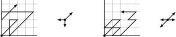
Figure 3: Left: example of Kreweras’ walk. Right: example of Gessel’s walk.

A more complicated case is random walks in $\mathbb{Z}^{3}$ constrained in a cone defined by $\theta<\theta_{\max}$ (in spherical coordinates). In this case, the survival probability is $F(t)\sim ct^{-\nu/2}$, where $\nu$ is the smallest positive number such that $P_{\nu}(\cos\theta_{\max})=0$, where $P_{\nu}$ is the Legendre function (Redner, 2001, Section 7.3). This allows for the exponent $\alpha=\nu/2$ to be any positive number. In particular, since $P_{2}(x)=(3x^{2}-1)/2$, an exponent $\alpha<1$, and thus a linear-time algorithm, is achieved for $\theta_{\max}>\arccos(1/\sqrt{3})$.

In fact, generic cones in generic dimensions, and for a large class of periodic lattices, can also be handled in this way. Full details can be found in Denisov and Wachtel (2015), and, in particular, their Section 1.2 illustrates the required precise technical assumptions. Let us summarise in few words these hypotheses. There are four of them. The first two are mild requests on the shape of the cone, which in particular are automatically satisfied in dimension 2. A third hypothesis allows for long-range walk steps, provided that certain moments are finite (we only considered walks with finite-range steps here). A fourth hypothesis requires that the associated unbounded random walks undergo isotropic diffusion, and always holds in absence of drift (as we require here for having non-trivial asymptotics), up to applying an appropriate affine transformation to the lattice.

Let $\Omega$ be a cone of $\mathbb{R}^{d}$ and let $\Omega_{0}=\Omega\cap\mathbb{S}^{d-1}$. Under the conditions detailed in the reference, the survival probability in the cone $\Omega$ satisfies:

$$F(t)\sim ct^{-\nu/2}\text{,}$$

where $\nu$ is the smallest positive number such that there exists a function $h_{\nu}(\theta)$ on the unit sphere vanishing at the border of $\Omega_{0}$ and satisfying:

$$\Delta_{S}h_{\nu}(\theta)=-\lambda h_{\nu}(\theta)\text{,}\qquad\qquad\lambda=\nu(\nu+d-2)\text{,}$$

where $\Delta_{S}$ is the spherical Laplace operator.

Thus, we are again in the conditions of Theorem 2.1, with $\alpha=\nu/2$. The exponent $\nu$ is, however, difficult to compute in general.

4.6 More complex random walk problems

In the previous section we considered random walks on a lattice that shall avoid some “wall” prescribed deterministically. Here we consider a more complex problem in which the growing structure produces the walls dynamically. Say that two paths on a graph intersect if they share some vertex. We have two classes of problems: (P1) a walk $\omega$ of length $n$, starting at a neighbour of the origin, such that there exists some infinite walk connecting the origin to infinity and not intersecting $\omega$. (P2) for $k\geq 2$, $k$-tuples of walks $(\omega_{1},\ldots,\omega_{k})$, of length $n$, starting from nearby vertices (e.g., aligned along a line), that shall not intersect each other.

For undirected random walks, the simplest lattice is $\mathbb{Z}^{D}$, i.e., with the $2D$ possible steps $\{s^{\alpha}\}=\{(0,0,\ldots,\pm 1,\ldots,0)\}$ uniformly chosen. The analogue for directed random walks is $\mathbb{N}\times\mathbb{Z}^{D-1}$, i.e., with the $2(D-1)$ possible steps $\{s^{\alpha}\}=\{(1,0,\ldots,\pm 1,\ldots,0)\}$ uniformly chosen. More generally, we may consider unbiased isotropic (undirected) random walks, i.e., walks that can perform steps $s^{\alpha}\in\mathbb{Z}^{D}$ with weight $w_{\alpha}$, such that $\sum_{\alpha}w_{\alpha}s_{i}^{\alpha}=0$ for all $i=1,\ldots,D$ and $\sum_{\alpha}w_{\alpha}s_{i}^{\alpha}s_{j}^{\alpha}=C\delta_{ij}$. In the directed variant we have $s_{1}^{\alpha}=1$ for all steps $\alpha$, and all other compatible constraints are left as are.

The associated exponents, when non-trivial (i.e., for $D$ sufficiently small), are in general hard to evaluate. For directed walks in $D=2$, (P1) is trivial, and (P2) is called vicious walkers. The well-known relation with classical ensembles of random matrices gives $\alpha=k(k-1)/4$ in that case. This means that we have no problems in the interesting range $0<\alpha<1$, except for $k=2$, which, on $\mathbb{N}\times\mathbb{Z}$, reduces to prefixes of Dyck paths through a simple bijection.

For undirected walks in $D=2$, conformal invariance, and even better the connection with the exactly solvable analysis on random planar graphs via KPZ relation (Knizhnik et al. (1988)), have led to the determination of a variety of critical exponents, which have been proven subsequently by SLE techniques (see Duplantier (1998) for the original conjectures, and Lawler et al. (2001a, b, 2002) for the proofs). As shown in Lawler et al. (2001b), we have $\alpha=\frac{1}{24}(4k^{2}-1)$, in a unified formula for (P1) (using $k=1$) and for (P2). Thus we have two new problems in the interesting range: problem (P1), following the law $\mathcal{D}(\frac{1}{8})$, and problem (P2) with $k=2$, following the law $\mathcal{D}(\frac{5}{8})$. An example of the latter is in Figure 4.

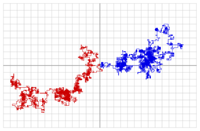
Figure 4: A random sampling of two walks, each of length $n=2000$, on $\mathbb{Z}^{2}$, starting at neighbouring points and avoiding each other.

References

- Bacher [2014] A. Bacher. Directed and multi-directed animals in the king’s lattice. Submitted, 2014. URL http://arxiv.org/abs/1301.1365.
- Bacher et al. [2014] A. Bacher, O. Bodini, and A. Jacquot. Efficient random sampling of binary and unary-binary trees via holonomic equations. Submitted, 2014. URL http://arxiv.org/abs/1401.1140.
- Banderier and Flajolet [2002] C. Banderier and P. Flajolet. Basic analytic combinatorics of directed lattice paths. Theoretical Computer Science, 281:37–80, 2002. (special volume dedicated to M. Nivat).
- Barcucci et al. [1994] E. Barcucci, R. Pinzani, and R. Sprugnoli. The random generation of directed animals. Theoret. Comput. Sci., 127(2):333–350, 1994.
- Barcucci et al. [1995] E. Barcucci, R. Pinzani, and R. Sprugnoli. The random generation of underdiagonal walks. Discrete Math., 139(1-3):3–18, 1995. Formal power series and algebraic combinatorics (Montreal, PQ, 1992).
- Bonichon [2002] N. Bonichon. Aspects algorithmiques et combinatoires des réaliseurs des graphes plans maximaux. PhD thesis, Université Sciences et Technologies – Bordeaux I, 2002.
- Bousquet-Mélou and Mishna [2010] M. Bousquet-Mélou and M. Mishna. Walks with small steps in the quarter plane. Contemp. Math., 520:1–40, 2010.
- Darling [1952] D. A. Darling. The influence of the maximum term in the addition of independent random variables. Trans. Amer. Math. Soc., 73:95–107, 1952.
- Denisov and Wachtel [2015] D. Denisov and V. Wachtel. Random walks in cones. The Annals of Probability, 43(3):992–1044, 2015. URL http://arxiv.org/abs/1110.1254.
- Duplantier [1998] B. Duplantier. Random walks and quantum gravity in two dimensions. Phys. Rev. Lett., 81:5489–5492, 1998. doi: 10.1103/PhysRevLett.81.5489. URL http://link.aps.org/doi/10.1103/PhysRevLett.81.5489.
- Gnedenko and Kolmogorov [1968] B. V. Gnedenko and A. N. Kolmogorov. Limit distributions for sums of independent random variables. Translated from the Russian, annotated, and revised by K. L. Chung. With appendices by J. L. Doob and P. L. Hsu. Revised edition. Addison-Wesley Publishing Co., Reading, Mass.-London-Don Mills., Ont., 1968.
- Knizhnik et al. [1988] V. G. Knizhnik, A. M. Polyakov, and A. B. Zamolodchikov. Fractal structure of -quantum gravity. Modern Physics Letters A, 03(08):819–826, 1988. URL http://www.worldscientific.com/doi/abs/10.1142/S0217732388000982.
- Lawler et al. [2001a] G. Lawler, O. Schramm, and W. Werner. Values of brownian intersection exponents, i: Half-plane exponents. Acta Mathematica, 187(2):237–273, 2001a. ISSN 0001-5962. doi: 10.1007/BF02392618. URL http://dx.doi.org/10.1007/BF02392618.
- Lawler et al. [2001b] G. Lawler, O. Schramm, and W. Werner. Values of brownian intersection exponents, ii: Plane exponents. Acta Mathematica, 187(2):275–308, 2001b. ISSN 0001-5962. doi: 10.1007/BF02392619. URL http://dx.doi.org/10.1007/BF02392619.
- Lawler et al. [2002] G. F. Lawler, O. Schramm, and W. Werner. Values of brownian intersection exponents iii: Two-sided exponents. Annales de l’Institut Henri Poincare (B) Probability and Statistics, 38(1):109 – 123, 2002.
- Lew [1994] J. S. Lew. On the Darling-Mandelbrot probability density and the zeros of some incomplete gamma functions. Constr. Approx., 10(1):15–30, 1994.
- Louchard [1999] G. Louchard. Asymptotic properties of some underdiagonal walks generation algorithms. Theoret. Comput. Sci., 218(2):249–262, 1999. Caen ’97.
- Penaud et al. [2001] J.-G. Penaud, E. Pergola, R. Pinzani, and O. Roques. Chemins de Schröder et hiérarchies aléatoires. Theoret. Comput. Sci., 255(1-2):345–361, 2001.
- Redner [2001] S. Redner. A guide to first-passage processes. Cambridge University Press, Cambridge, 2001.