An adaptive kriging method for solving nonlinear inverse statistical problems

Abstract

In various industrial contexts, estimating the distribution of unobserved random vectors $X_{i}$ from some noisy indirect observations $H(X_{i})+U_{i}$ is required. If the relation between $X_{i}$ and the quantity $H(X_{i})$, measured with the error $U_{i}$, is implemented by a CPU-consuming computer model $H$, a major practical difficulty is to perform the statistical inference with a relatively small number of runs of $H$. Following Fu et al., [13], a Bayesian statistical framework is considered to make use of possible prior knowledge on the parameters of the distribution of the $X_{i}$, which is assumed Gaussian. Moreover, a Markov Chain Monte Carlo (MCMC) algorithm is carried out to estimate their posterior distribution by replacing $H$ by a kriging metamodel build from a limited number of simulated experiments. Two heuristics, involving two different criteria to be optimized, are proposed to sequentially design these computer experiments in the limits of a given computational budget. The first criterion is a Weighted Integrated Mean Square Error (WIMSE) [28]. The second one, called Expected Conditional Divergence (ECD), developed in the spirit of the Stepwise Uncertainty Reduction (SUR) criterion [41, 5], is based on the discrepancy between two consecutive approximations of the target posterior distribution. Several numerical comparisons conducted over a toy example then a motivating real case-study show that such adaptive designs can significantly outperform the classical choice of a maximin Latin Hypercube Design (LHD) of experiments. Dealing with a major concern in hydraulic engineering, a particular emphasis is placed upon the prior elicitation of the case-study, highlighting the overall feasibility of the methodology. Faster convergences and manageability considerations lead to recommend the use of the ECD criterion in practical applications.

Keywords: Inverse statistical problems; Bayesian inference; Kriging; Adaptive design of experiments; Metropolis-Hasting-within-Gibbs algorithm; Prior elicitation.

1 Introduction

In many industrial problems, engineers have to deal with uncertain quantities which cannot be directly measured. Moreover, some of them can suffer from some inherent variability. For instance, in hydraulics, the assessment of a risk of flooding usually depends on some quantities, called coefficients of Manning-Strickler, which represent the roughness of the river bed. Because rivers are complex changeable systems, it appears reasonable to consider these coefficients as random variables. Although they cannot be directly measured, it appears possible to estimate their randomness from flooding data by means of computer simulation.

Estimating the probability distribution of such random unobserved variables involves some observations $Y_{i}\in\mathbb{R}^{p}$ (e.g., water levels), $i=1\ldots{}n$, and a computer model $H$ (e.g., Saint-Venant equation solver) which links the unobserved variables of interest $X_{i}\in\mathbb{R}^{q}$ (e.g., Manning-Strickler coefficients) to the $Y_{i}$:

$$Y_{i}=H(X_{i},d_{i})+U_{i}$$ (1)

where $d_{i}\in\mathbb{R}^{q_{2}}$ stands for some known or observed quantities and where $U_{i}$ represents some unobserved measurement errors. A Gaussian framework is adopted in this article: the ${(X_{i}\;U_{i})}^{T}$ are assumed to be independent Gaussian random vectors such that

$$\left(\begin{array}[]{c}X_{i}\\ U_{i}\end{array}\right)\sim\mathcal{N}_{q+p}(\left(\begin{array}[]{c}m\\ 0\end{array}\right),\left(\begin{array}[]{cc}C&0\\ 0&R\end{array}\right))$$ (8)

where $\mathcal{N}_{k}(\mu,\Sigma)$ is the $k$-dimensional Gaussian distribution of mean $\mu$ and covariance matrix $\Sigma$. The issue is then to estimate the unknown parameters $\theta=(m,C)$ of the probability distribution of the $X_{i}$ from some field data $(y_{i},d_{i})$, $1\leq i\leq n$, given $H$ and the error covariances $R$. The accuracy of measurements is generally given or can be assessed: the assumption that $R$ is known is a sound basis for the inference, since it prevents from a problem of non-identifiability of ($\theta,R$).

From the general perspective of the analysis of some independent measurements $y_{i}$ performed on similar systems (under conditions $d_{i}$), this statistical model enables to capture the inherent variability of some variables $X_{i}$ in the population which is studied. For instance, mechanical tests generally involve a production-lot population of components whose precise characteristics (e.g. Young’s Modulus or thermal expansion coefficient) suffer from a non negligible variability.

The major practical obstacle to the estimation of $\theta$ is the CPU cost and time needed to evaluate $H(x,d)$, given an input $(x,d)\in\mathbb{R}^{Q}$ ($Q=q+q_{2}$). In hydraulics, one run of $H$ takes typically few hours per CPU. Several methods have been developed to tackle this difficulty. Celeux et al., [11] considered a maximum likelihood estimation by Expectation-Conditional Maximisation Either (ECME) [21] based on an iterative linearisation of $H$: this algorithm should be avoided if the nonlinearities of $H$ relative to $x$ are significant, otherwise it can be very efficient. Barbillon et al., [2] proposed to couple a Stochastic Expectation Maximisation (SEM) algorithm [10] with a kriging metamodelling of $H$ to improve the robustness of the estimation.

Kriging, also known as Gaussian Process (GP) regression, was suggested by Sacks et al., [31] to deal with CPU-expensive computer models. The purpose of this metamodelling technique is to build an accurate surrogate model of $H$ from some computer experiments (some runs of $H$). Then a crucial question is how to determine the Design of these Experiments (DoE). Several methods of calibration of computer models relying on kriging were proposed by Kennedy and O’Hagan, [18] and Bayarri et al., [4]. Although their statistical models are close to the one postulated here, an important difference is that the $X_{i}$ are assumed to be random in this article, whereas the unknown inputs $x$ are part of the parameters $\theta$ to estimate in their studies.

Hereafter, the Bayesian framework suggested by Fu et al., [13], which involves a kriging of $H$, is considered. It allows to take account of prior information about the $X_{i}$ (which could possibly arise from expert or past assessments) through the definition of a so-called prior probability distribution for $\theta$, the density of which being denoted $\pi(\theta)$. A Metropolis-Hastings-within-Gibbs Markov Chain Monte-Carlo (MCMC) sampling can then be carried out to estimate the posterior distribution of $\theta$ (given the field data). The benefit of kriging is twofold: extensive sampling gets feasible, and the uncertainty about $H$ can be accounted for by embedding the GP into the statistical model and the MCMC procedure.

From a Bayesian point of view, there is no reason to drop the uncertainty on $H$ by only keeping the kriging predictor $\hat{H}(.)$. Besides, the development of purpose-oriented adaptive DoE approaches, such as the Stepwise Uncertainty Reduction (SUR) [41, 5], is then made possible. Such approaches seek a trade-off between shrinking the uncertainty on $H$ (which is measured by the kriging covariance) as much as possible, and exploring the most interesting areas of the input space of $H$ regarding the considered objective. A classical example comes from the field of global optimisation where the Expected Improvement criteria was proposed by Mockus et al., [25], Jones et al., [17]. The purpose of this article is to contribute to the definition of efficient adaptive DoE algorithms for solving the inverse statistical problem specified earlier.

The article is organised as follows. Section 2 gives details about kriging metamodelling, as well as the maximin Latin Hypercube Design (maximin LHD) which provides us with a first knowledge about the computer model $H$ (before starting a purpose-oriented exploration of the input space of $H$). In Section 3, the method used to specify an informative prior $\pi(\theta)$, then the inference by MCMC, are described. Afterwards, two methods, called Expected Conditional Divergence (ECD) and Weighted Integrated Mean Square Error (WIMSE), which derive from two purpose-oriented criteria to optimise, are proposed to sequentially enrich the DoE in Section 4 and Section 5. Numerical studies are conducted on on toy example in Section 6 to compare the efficiency of these approaches with a posterior approximation standed on a static space-filling design (maximin LHD). Finally, the full methodology is run through over a real hydraulic computer model: its input roughness parameters are calibrated from noisy observations of water levels. Section 8 concludes the article by giving major directions for further work.

2 Kriging and maximin LHD space-filling design

This section recall some basics of kriging and of designing computer experiments which matter for the remainder of the article.

2.1 Kriging

Kriging is a geostatistical method [23] which was suggested by Sacks et al., [31] to build a cheap surrogate model of a computer model, from a limited of runs of the latter, over a hypercube $\Omega\subset\mathbb{R}^{Q}$. This method has known a growing interest in metamodelling with the writings of Koehler and Owen, [20], Stein, [35], Kennedy and O’Hagan, [18], Santner et al., [32], amongst others. In this section, a scalar function $h:\Omega\rightarrow\mathbb{R}$ is considered: in the case of a vector-valued function $H:\Omega\rightarrow\mathbb{R}^{p}$, each component $h_{i}(.)$ of $H(.)$ can be “kriged” independently from the others, as done in the numerical experiments in Section 6.

A usual manner to present kriging is starting from the premise that the considered function $h(.)$ is a particular realization of an underlying GP $\mathcal{H}(.)$:

$$\forall z\in\Omega, \mathcal{H}(z)=F(z)\,\beta+\mathcal{G}(z),$$ (9)

where $\beta$ is a vector of $\mathbb{R}^{K}$, where $F(z)=\left(\begin{array}[]{c}\!\!f_{1}(z)\cdots f_{K}(z)\!\!\end{array}\right)$ with $f_{k}:\mathbb{R}^{Q}\rightarrow\mathbb{R}^{p}$, $1\leq k\leq K$, a family of linearly independent functions, and where $\mathcal{G}$ is a centered GP ($\mathbb{E}\left[{\mathcal{G}(z)}\right]=0$, for all $z\in\Omega$). The GP hypothesis means that ${\left(\begin{array}[]{c}\!\!\mathcal{G}(z_{1})\>\cdots\>\mathcal{G}(z_{k})\!\!\end{array}\right)}^{T}$ is a $k$-dimensional Gaussian vector for any set $\{z_{1},\cdots,z_{k}\}\in\Omega$ and any $k\geq 1$. Although it may appear artificial, this assumption leads to a flexible statistical model which has been applied successfully in many contexts, and, in a Bayesian perspective, it can be interpreted as the definition of a prior on $h$ [30]. For any $(z,w)\in\Omega^{2}$, the mean function $\mu:\Omega\rightarrow\mathbb{R}$ of $\mathcal{H}$ is defined by $\mu(z)=\mathbb{E}\left[{\mathcal{H}(z)}\right]=F_{z}\,\beta$, and the covariance function $K:\Omega^{2}\rightarrow\mathbb{R}$ of $\mathcal{G}$ (and $\mathcal{H}$) by $\mbox{Cov}\left[{\mathcal{G}(z),\mathcal{G}(w)}\right]=K(z,w)$. In the following, as most often assumed by authors when modelling computer models, $\mathcal{G}$ is stationary, thus $K(z,w)$ only depends on $z-w$: $K(z,w)=\sigma^{2}\,K(z-w)$ by abuse of notation, with $K(0)=1$.

Let $D_{N}=\{z_{1},\cdots,z_{N}\}\subset\Omega$ be a DoE associated to observations $h_{N}\in\mathbb{R}^{N}$, and ${\mathcal{H}_{N}}^{T}=\left(\begin{array}[]{c}\!\!\mathcal{H}(z_{1})\cdots\mathcal{H}(z_{N})\!\!\end{array}\right)$, then, from a direct application of a classical theorem relative to the conditioning of Gaussian vectors, the process $\mathcal{H}$ conditioned by the observations, that is $\mathcal{H}|\mathcal{H}_{N}\!=\!h_{N}$, is still a GP over $\Omega$ with mean function $\mu_{D_{N}}:\Omega\rightarrow\mathbb{R}$ and covariance function $K_{D_{N}}:\Omega^{2}\rightarrow\mathbb{R}$. Namely, for all $(z,w)$,

$$h_{N}(z) \sim {\cal{N}}\left(\mu_{D_{N}}(z),{K_{D_{N}}(z,\cdot)}\right)$$ (10)

where

$$\mu_{D_{N}}(z)=F(z)\,\beta+K_{z,N}{K_{N,N}}^{-1}(h_{N}\!-\!F_{N}\,\beta)$$ (11)

$$K_{D_{N}}(z,w)=K(z,w)-K_{z,N}{K_{N,N}}^{-1}{K_{w,N}}^{T}$$ (12)

with $K_{z,N}=\left(\begin{array}[]{c}\!\!K(z,z_{1})\cdots K(z,z_{N})\!\!\end{array}\right)$ (idem for $K_{w,N}$) and ${[K_{N,N}]}_{i,j}=K(z_{i},z_{j})$. Of course, $K_{D_{N}}(z,z)<K(z,z)$: the more observations are available, the less uncertainty on $\mathcal{H}$ remains. If $K(.,.)$ and $\beta$ are known, then $\mu_{D_{N}}(z)$ is the kriging predictor of $\mathcal{H}(z)|\mathcal{H}_{N}\!=\!h_{N}$, that is its Best Linear Unbiaised Predictor (BLUP), and $K_{D_{N}}(z,w)$ is the kriging covariance, that is the covariance function of the error of prediction. In particular, $K_{D_{N}}(z,z)$ is the Mean Square Error (MSE) of the BLUP at $z$.

Furthermore, if $K(.,.)$ is known but $\beta$ unknown (universal kriging), then the generalised least-square estimator

$$\hat{\beta}={({F_{N}}^{T}K_{N,N}F_{N})}^{-1}{F_{N}}^{T}K_{N,N}h_{N}$$ (13)

of $\beta$ is also the maximum likelihood estimator, and the BLUP $\hat{h}_{D_{N}}(z)$ of $\mathcal{H}(z)|\mathcal{H}_{N}\!=\!h_{N}$ is obtained by substituting $\beta$ by $\hat{\beta}$ in Equation (11). Last but not least, the kriging covariance which is associated to $\hat{h}_{D_{N}}(z)$ is then

$$K_{D_{N}}(z,w) = K(z,w)-K_{z,N}{K_{N,N}}^{-1}{K_{w,N}}^{T}$$

$$+ {(F(z)-{F_{N}}^{T}{K_{N,N}}^{-1}{K_{z,N}}^{T})}^{T}{({F_{N}}^{T}{K_{N,N}}^{-1}F_{N})}^{-1}$$

$$\ \ \times\ (F(w)-{F_{N}}^{T}{K_{N,N}}^{-1}{K_{w,N}}^{T})$$

(we use the same notation as before - $\beta$ known - for the sake of simplicity) with $[{F_{N}}]_{i,j}=f_{j}(z_{i})$. It can be seen as an approximation of the covariance function of the GP $\mathcal{H}|\mathcal{H}_{N}\!=\!h_{N}$ and, together with $\hat{h}_{D_{N}}(z)$, is generally used, for example in [5], to model the uncertainty on the Gaussian vector ${\left(\begin{array}[]{c}\!\!\mathcal{H}(w_{1})\cdots\mathcal{H}(w_{M})\end{array}\right)}^{T}|\mathcal{H}_{N}\!=\!h_{N}$ for any set $\{w_{1},\cdots,w_{M}\}\subset\Omega$; see also Santner et al., [32], Bachoc, [1] for other precisions. Following Fu et al., [13], $K_{D_{N}}(z,w)$ is used in the MCMC procedure to account for the dependence between the missing data $X_{i}$ due to the uncertainty on (each component $h_{i}(.)$ of) the computer model $H(.)$; see Section 3 for more details. The induced Mean Square Error $MSE_{D_{N}}:z\mapsto K_{D_{N}}(z,z)$ plays an important role in Section 5.

In practical applications, $K(.,.)$ is unknown and is estimated, thanks to a model $K_{\psi}(.,.)$ parametrised by $\psi\in\mathbb{R}^{L}$, by different techniques such as maximum likelihood (as hereafter) or cross-validation. In the remainder of this article, the plug-in estimates obtained by replacing $K(.,.)$ by $K_{\hat{\psi}}(.,.)$, with $\hat{\psi}$ the estimator of $\psi$, are employed.

2.2 Design of experiments (maximin-Latin Hypercubic Designs)

Obviously, the predicting accuracy of kriging highly depends on the DoE $D_{N}$. Following Picheny et al., [28], it is possible to distinguish three kinds of DoEs:

• space-filling designs, which aim to fill the input space with a finite number of points independently of the considered model (e.g., maximin-LHD);

• model-oriented designs, which attempt to build a suited DoE accounting for the features of the model $H$ or the metamodel (e.g. IMSE, see Section 5.1);

• purpose-oriented designs, which account for the final aim of the study to find the best adapted DoE (e.g., to compute an exceedance probability by accelerated Monte Carlo methods).

In this article, a purpose-oriented DoE is built in an adaptive way. A first calibration of the covariance parameters is performed from an initial maximin-LHD, then the DoE is sequentially improved using sequential strategies, which are detailed in sections 4 and 5. The concept of LHDs was introduced in [24]; such designs ensure a good coverage of the interval to which each scalar variable belongs. Then [16] proposed the maximin distance criterion to optimize LHDs. Maximin means maximizing the minimum inter-site distance between the set of $N$ points:

$$\delta_{D} = \min_{i\neq j}\|z_{(i)}-z_{(j)}\|_{2}.$$

Therefore, the maximin criterion prevents the points of the design to be close to each other. In the present work, maximin-LHDs are obtained by the algorithm of Morris and Mitchell, [26].

3 Bayesian statement and inference

3.1 Prior elicitation

In the Bayesian statistical framework favored in [13], a Gaussian-Inverse Wishart prior distribution was elicited:

$$m\,|\,C \sim \mathcal{N}_{q}(\mu,C/a),$$ (15)

$$C \sim \mathcal{IW}_{q}(\Lambda,\nu).$$ (16)

This prior can be assimilated to the posterior distribution of virtual data given a noninformative prior, which presents some advantages in subjective Bayesian analysis [8]. Especially, a clear sense can be given to hyperparameters $(\mu,a,\Lambda,\nu)$, which simplifies prior calibration.

Indeed, $a$ can be understood as the size of virtual sample of data $X$, that modulates the strength of the practicioner’s belief in prior information (for instance provided by subjective experts). It should be calibrated under the constraint $a<n$ to ensure that the posterior behavior is mainly driven by objective data information. A default (let say, “objective”) choice is $a=1$.

Furthermore, $\mu$ is the prior predictive mean, median and most probable value of $X$, which can be estimated by a measure of central tendency provided by past calibration results in close situations. In the motivating case-study explored in Section 7, such information was found by bibliographical researches (Table 3).

Finally, denoting $\mathbf{X,Y}$ the set of missing and truly observed data, the reparametrizations $\Lambda=(a+1)\cdot C_{e}$ and $\nu=a+q+2$ imply that the conditional posterior distribution of $C$ given $m$ is the Inverse Wishart distribution $\mathcal{IW}\Big{(}(a+1)\,C_{e}+(n+1)\,\hat{C}_{n},\,\nu+n+1\Big{)}$ with $\hat{C}_{n}=\frac{1}{n}\sum_{i=1}^{n}(m-x_{i})(m-x_{i})^{T}$, the expectation of which being

$$\mathbb{E}[C\,|\,m,\mathbf{X,Y}] = \frac{a+1}{a+n+2}\cdot C_{e}+\frac{n+1}{a+n+2}\cdot\hat{C}_{n}.$$

This last expression highlights the meaning and influence of $a$ as a virtual size. The components of $C_{e}$ are to be calibrated in function of prior knowledge on $X$ too, expressed through its predictive prior distribution, which is a decentered Student law:

$$X \sim \mbox{St}_{q}\Big{(}\mu,\,\frac{(a+1)^{2}}{a(a+3)}C_{e},\,a+3\Big{)}$$

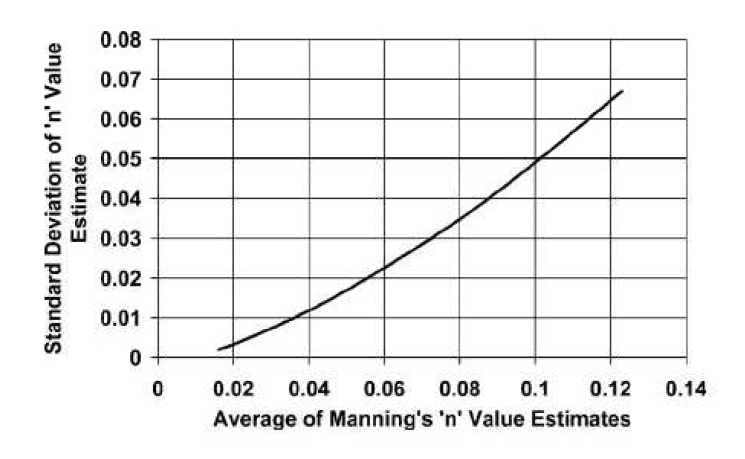
Figure 6: Uncertainty over the estimators of Manning coefficient ($M=1/X$), from of Engineers, [27]. Cited (Fig. 3.5) in Liu, [22].

with mean vector $\mu$ and covariance matrix $\frac{a+1}{a}C_{e}$. Again, in the case-study that motivated this work, prior information on the ratio between average values and standard deviation of Strickler-Manning coefficients was available (Figure 6), which allowed for a full prior calibration (Section 7).

3.2 Posterior computation

A Gibbs sampler [37] was proposed to compute the posterior distribution of $\theta=(m,C)$. Actually, replacing the expensive-to-compute function $H$ with a kriging emulator $\widehat{H}$, as in Barbillon et al., [2], and introducing a new emulator error MSE, the Gibbs sampler can be adapted as follows:

Gibbs sampler (at the $(r+1)$-th iteration)

 

Given $(m^{(r)},C^{(r)},\mathbf{X}^{(r)})$ for $r=0,1,2,\dots$, generate:

1. $C^{(r+1)}|\dots\sim\mathcal{IW}\Big{(}\Lambda+\sum_{i=1}^{n}(m^{(r)}-X_{i}^{(r)})(m^{(r)}-X_{i}^{(r)})^{\prime}+a(m^{(r)}-\mu)(m^{(r)}-\mu)^{\prime},\,\nu+n+1\Big{)}$,

2. $m^{(r+1)}|\dots\sim\mathcal{N}\Big{(}\frac{a}{n+a}\mu+\frac{n}{n+a}\overline{\mathbf{X}_{n}^{(r)}},\,\frac{C^{(r+1)}}{n+a}\Big{)}$ where $\overline{\mathbf{X}_{n}^{(r)}}=n^{-1}\sum_{i=1}^{n}X_{i}^{(r)}$,

3. $\mathbf{X}^{(r+1)}|\dots\propto|\mathbf{R}+\mbox{MSE}^{(r+1)}|^{-\frac{1}{2}}\cdot\exp\Bigg{\{}-\frac{1}{2}\sum_{i=1}^{n}(X_{i}^{(r+1)}-m^{(r+1)})^{\prime}\Big{[}C^{(r+1)}\Big{]}^{-1}(X_{i}^{(r+1)}-m^{(r+1)})-\frac{1}{2}\Big{(}\Big{(}\mathcal{Y}_{1}-\widehat{H}_{N,1}^{(r+1)}\Big{)}^{\prime},\dots,\Big{(}\mathcal{Y}_{n}-\widehat{H}_{N,n}^{(r+1)}\Big{)}^{\prime}\Big{)}\Big{(}\mathbf{R}+\mbox{MSE}^{(r+1)}\Big{)}^{-1}\left(\begin{array}[]{c}\mathcal{Y}_{1}-\widehat{H}_{N,1}^{(r+1)}\\ \vdots\\ \mathcal{Y}_{n}-\widehat{H}_{N,n}^{(r+1)}\end{array}\right)\Bigg{\}}\\$

   where $\widehat{H}_{N,i}^{(r+1)}=\widehat{H}_{N}(X_{i}^{(r+1)},d_{i})$ and $\mbox{MSE}^{(r+1)}=\mbox{MSE}(\mathbf{X}^{(r+1)},\mathbf{d})$ is the block diagonal matrix

   $$\mathbf{\mbox{MSE}}(\mathbf{X}^{(r+1)},\mathbf{d}) = \begin{array}[]{cl}\left(\begin{array}[]{ccc}\mbox{MSE}_{1}(\mathbf{X}^{(r+1)},\mathbf{d})&&{\bf 0}\\ &\ddots&\\ {\bf 0}&&\mbox{MSE}_{p}(\mathbf{X}^{(r+1)},\mathbf{d})\end{array}\right)&\begin{array}[]{ll}\left.\begin{array}[]{l}\\ \end{array}\right\}&n\textrm{ lines}\\ \\ \left.\begin{array}[]{l}\\ \end{array}\right\}&n\textrm{ lines}\\ \end{array}\end{array}$$

 

In the third step, the variance matrices $\mbox{MSE}_{j}(\mathbf{X}^{(r+1)},\mathbf{d})\in\mathcal{M}^{n\times n}$ are defined by

$$\mbox{MSE}_{j}(\mathbf{X}^{(r+1)},\mathbf{d}) = \mathbb{E}\left(\left(\mathcal{H}_{j}(\mathbf{X}^{(r+1)},\mathbf{d})-\widehat{H}_{j}(\mathbf{X}^{(r+1)},\mathbf{d})\right)^{2}\,|\,\mathbf{H}_{D_{N}}\right),$$

for $j=1,\ldots,p$, where $\mathcal{H}_{j}$ denotes the $j$-th dimension of the Gaussian process $\mathcal{H}$. Moreover,

$$\mathbf{R} = \begin{array}[]{cl}\left(\begin{array}[]{ccc}\mathbf{R}_{1}&&{\bf 0}\\ &\ddots&\\ {\bf 0}&&\mathbf{R}_{p}\end{array}\right)&\begin{array}[]{ll}\left.\begin{array}[]{l}\\ \end{array}\right\}&n\textrm{ lines}\\ \\ \left.\begin{array}[]{l}\\ \end{array}\right\}&n\textrm{ lines}\\ \end{array}\end{array},\textrm{ with }\,\mathbf{R}_{i}\,=\,\left(\begin{array}[]{ccc}R_{ii}&&0\\ &\ddots&\\ 0&&R_{ii}\end{array}\right),$$

where $R_{ii}$ is the $i-$th diagonal component of the diagonal variance matrix $R$. It is worth noting that this third conditional distribution does not belong to any closed form family of distributions. Therefore a Metropolis-Hastings (MH) step is used to simulate $\mathbf{X}^{(r+1)}$ (see Appendix A).

As discussed in [13], the use of the MCMC algorithms involves many possible errors. According to experimental trials, the accuracy of the metamodel plays a critical role in the the estimation problem. MCMC algorithms can produce Markov chains converging towards the desired posterior distribution. However, if the function $H$ is really badly approximated, apart from the algorithmic error introduced by the MCMC algorithm, the result can also suffer from an emulator error.

4 The Expected Conditional Divergence criterion for adaptive designs

The two following sections address the issue of building adaptive designs of experiments, by proposing two strategies. In this section, a criterion called ECD (Expected Conditional Divergence) is built, which can be seen as an adaptation of the Expected Improvement criterion proposed in Jones et al., [17]. Let us notice that the expected divergence criterion proposed in the next section, although close to a Stepwise Uncertainty Reduction (SUR) criterion, does not derive from the SUR formulation of Vazquez and Bect, [41], Bect et al., [5]. The latter would lead to a more challenging approach from a computational perspective in our context.

4.1 Principle

Ideally, the posterior distribution of the parameters $\theta=(m,C)$ after adding a new point $z_{(N+1)}$ to the current DoE $D_{N}$ should be as close as possible to the posterior distribution knowing the original function $H$, i.e. a relevant discrepancy measure between the two relative distributions must be minimized. Based on information-theoretical arguments given in Cover and Thomas, [12], the Kullback-Leibler (KL) divergence

$$\mbox{KL}\Big{(}\pi(\theta|{\bf y,d},H)\,||\,\pi(\theta|{\bf y,d},\mathbf{H}_{D_{N}}\cup\{H(z)\}))\Big{)},$$ (25)

is a good choice of discrepancy measure. Remind that given two densities $p(x)$ and $q(x)$ defined over the same space $\mathcal{X}$,

$$\mbox{KL}(p||q) = \int_{\mathcal{X}}p(x)\log\frac{p(x)}{q(x)}\,dx.$$

Ideally, the next point $z_{(N+1)}$ should be searched within the feasible region $\Omega$, as the global minimum of this divergence. But obviously, the unknown term $\pi(\theta|{\bf y,d},H)$ makes this formulation intractable. But a tractable sub-optimal criterion can be heuristically derived from it by the following rationale. It must be noticed that

$$z_{(N+1)} = \smash{\mathop{{\rm argmin}}\limits_{z\in\Omega}}\,\,\mbox{KL}\Big{(}\pi(\theta|{\bf y,d},H)\,||\,\pi(\theta|{\bf y,d},\mathbf{H}_{D_{N}}\cup\{H(z)\})\Big{)},$$

$$= \smash{\mathop{{\rm argmin}}\limits_{z\in\Omega}}\,\,\mbox{KL}\Big{(}\pi(\theta|{\bf y,d},H)\,||\,\pi(\theta|{\bf y,d},\mathbf{H}_{D_{N}}\cup\{H(z)\})\Big{)}$$

$$\ \ \ -\ \mbox{KL}\Big{(}\pi(\theta|{\bf y,d},H)\,||\,\pi(\theta|{\bf y,d},\mathbf{H}_{D_{N}})\Big{)},$$

$$= \smash{\mathop{{\rm argmax}}\limits_{z\in\Omega}}\,\,\int_{\theta\in\Omega}\pi(\theta|{\bf y,d},H)\,\log\frac{\pi(\theta|{\bf y,d},\mathbf{H}_{D_{N}}\cup\{H(z)\})}{\pi(\theta|{\bf y,d},\mathbf{H}_{D_{N}})}\,d\theta.$$

The intractable target density $\pi(\theta|{\bf y,d},H)$ has to be replaced with its best available approximation, which is $\pi(\theta|{\bf y,d},\mathbf{H}_{D_{N}}\cup\{H(z)\})$. Under the kriging assumptions, for any $z$ this distribution is closer of $\pi(\theta|{\bf y,d},H)$ than $\pi(\theta|{\bf y,d},\mathbf{H}_{D_{N}})$. Therefore, a sub-optimal version of the idealistic criterion is:

$$z_{(N+1)} = \smash{\mathop{{\rm argmax}}\limits_{z\in\Omega}}\,\,\mbox{KL}\Big{(}\pi(\theta|{\bf y,d},\mathbf{H}_{D_{N}}\cup\{H(z)\})\,||\,\pi(\theta|{\bf y,d},\mathbf{H}_{D_{N}})\Big{)}.$$

In other words, the chosen strategy aims at finding the optimal point $z_{(N+1)}$ which modifies the actual distribution $\pi(\theta|{\bf y,d},\mathbf{H}_{D_{N}})$ as much as possible in an information-theoretic sense. First proposed by Stein, [34] as a loss function, the dissymetric KL divergence between the two consecutive posterior distributions, which is invariant under one-to-one transformation of the random vector $\theta$, has an operative interpretation as the loss of information (in natural information units or nits) which may be expected by choosing the baddest approximation $\pi(\theta|{\bf y,d},\mathbf{H}_{D_{N}})$ instead of the best (available) $\pi(\theta|{\bf y,d},\mathbf{H}_{D_{N}}\cup\{H(z)\})$ [12, 6].

The preceding formulation is not satisfactory yet, since one evaluation of the criterion requires one evaluation of $H$, which is time-consuming. However, in the spirit of EGO, it is possible to derive a new criterion considering the following Gaussian process based on the available observations $\mathbf{H}_{D_{N}}$ instead of $H$:

$$h_{N}(z) := \mathcal{H}(z)\,|\,\mathbf{H}_{D_{N}},$$ (26)

which follows the normal distribution given in (10). Thus, we define the expected divergence criterion:

$$z_{(N+1)} = \smash{\mathop{{\rm argmax}}\limits_{z\in\Omega}}\,\mathbb{E}_{\pi(h_{N})}\left[\mbox{KL}\left(\pi(\theta|{\bf y,d},\mathbf{H}_{D_{N}}\cup\{h_{N}(z)\})\,\right.\right.$$

$$\hskip 99.58464pt\left.\left.||\,\pi(\theta|{\bf y,d},\mathbf{H}_{D_{N}})\right)\right].\hskip 42.67912pt$$

The idea of considering the Gaussian variable $h_{N}(z)$ rather than the predictor $\widehat{H}_{N}(z)$ allows to account for the uncertainty introduced by the kriging methodology, while it requires usual Monte Carlo methods to approximate the double integrals, i.e. the expectation and the KL divergence.

Even if no run of $H$ is required, the evaluation of this expected divergence criterion requires many calculations. In the next section, a heuristic is proposed to shrink the computational cost of the approach.

4.2 The Expected Conditional Divergence heuristic

Preliminary experiments showed that the criterion defined in (4.1) is generally too expensive to be useful, except for extremely CPU-consuming code $H$. The main reason is that any test of a new point $z$ requires to run a Gibbs sampler. Therefore a last adaptation of the criterion is proposed: the Expected Conditional Divergence (ECD) criterion depends only on the intermediate full-conditional posterior distributions of $\theta$. More precisely, at the $(r+1)$-th iteration of the Metropolis-Hastings-within-Gibbs algorithm, the strategy is defined as:

$$z_{(N+1)} = \smash{\mathop{{\rm argmax}}\limits_{z\in\Omega}}\,\mbox{ECD}(z)$$ (28)

with

$$\mbox{ECD}(z) = \mathbb{E}_{\pi(h_{N})}\left[\mbox{KL}\Big{(}\pi(\theta|\tilde{\mathbf{X}}^{(r+1)}(z))\,||\,\pi(\theta|\mathbf{X}^{(r+1)})\Big{)}\right],$$ (29)

where $\mathbf{X}^{(r+1)}$ and $\tilde{\mathbf{X}}^{(r+1)}(z)$ denote the missing data samples simulated from

$$\mathbf{X}^{(r+1)} \sim \pi\left(\cdot|{\bf y,d},\theta^{(r+1)},\mathbf{H}_{D_{N}}\right),$$

$$\tilde{\mathbf{X}}^{(r+1)}(z) \sim \pi\left(\cdot|{\bf y,d},\theta^{(r+1)},\mathbf{H}_{D_{N}}\cup\{h_{N}(z)\}\right).$$

It is worth noting that in the ECD criterion, the final posterior distribution of $\theta$ is replaced by its sequential conditional posterior distribution at the $(r+1)$-th iteration. At the $(r+1)$-th iteration of the Gibbs sampling, given a candidate $z$ to enrich the DoE, this heuristic enables to compute a value $\mbox{ECD}(z)$ which is likely a sufficient approximation of the expected divergence criterion for the global algorithm to perform well. Moreover, once $\mbox{ECD}(z)$ has been evaluated, the computation of $\mbox{ECD}(z^{\prime})$ at a new candidate $z^{\prime}$ takes benefit of the computations performed during the calculation of $\mbox{ECD}(z)$ (sampling of $\mathbf{X}^{(r+1)}$ by Metropolis-Hastings, then sampling of $\theta$ given $\mathbf{X}^{(r+1)}$) and does not require a full Gibbs sampling anymore (just the MCMC sampling of $\tilde{\mathbf{X}}^{(r+1)}(z)$, then the sampling of $\theta$ given $\tilde{\mathbf{X}}^{(r+1)}(z)$). Hence it allows an exploration of the input space (optimization of ECD) for a acceptable CPU-cost.

Finally, using a standard Monte-Carlo estimator to estimate the expectation of the KL divergence according to $\pi(h_{N})$ (see (29)), the ECD heuristic algorithm proceeds as follows:

ECD strategy

   
Given $(m^{(0)},C^{(0)},\mathbf{X}^{(0)})$, an initial design $D_{N}$ with the corresponding evaluations $\mathbf{H}_{D_{N}}$ of $H$:

1. $r:=0$.

2. Perform $k$ new Gibbs iterations (Section 3.2); $r:=r+k$: this gives $\theta^{(r+1)}$.

3. Sample $\mathbf{X}^{(r+1)}$ from $\pi\left(\cdot|{\bf y,d},\theta^{(r+1)},\mathbf{H}_{D_{N}}\right)$ (see Appendix A).

4. Sample $\Upsilon=\{\theta_{1},\dots,\theta_{L_{2}}\}$ from $\pi(\cdot|\mathbf{X}^{(r+1)},{\bf y,d})$ (explicit distribution: see steps 1 and 2 of Section 3.2).

5. Get a new point $z_{(N+1)}$ to enrich the DoE by the optimization of ECD (simulated annealing, see Appendix C): for any $z$, assess $\mbox{ECD}(z)$ if needed by:

   1. Generate $M$ samples $(h^{1}_{N}(z),\dots,h^{M}_{N}(z))$ according to (26) and build $M$ corresponding emulators $(\widehat{H}^{1}_{N+1}(z),\dots,\widehat{H}^{M}_{N+1}(z))$ with $\widehat{H}^{i}_{N+1}(z)$ based on the dataset $\mathbf{H}_{D_{N}}\cup\{h^{i}_{N}(z)\}$ (no re-estimation of the covariance function parameters $\psi$, see Section 2.1).

   2. for $1\leq i\leq M$,

      (i)

      Sample $\tilde{\mathbf{X}}^{(r+1),i}(z)$ from $\pi(\cdot|{\bf y,d},\theta^{(r+1)},\widehat{H}^{i}_{N+1}(z))$ (see Appendix A).

      (ii)

      Sample $\Theta^{i}=\{\theta^{i}_{1},\dots,\theta^{i}_{L_{1}}\}$ with $\theta=(m_{1},\dots,m_{q},C_{11},\dots,C_{qq})$ from $\pi(\cdot|\tilde{\mathbf{X}}^{(r+1),i}(z),{\bf y,d})$(explicit distribution: see steps 1 and 2 of Section 3.2).

   3. $ECD(z):=\frac{1}{M}\sum_{i=1}^{M}\widehat{\mbox{KL}}\Big{(}\Theta^{i}\,||\,\Upsilon\Big{)}$ where $\widehat{\mbox{KL}}(.||.)$ denotes the KL divergence estimate (see Appendix B).

6. $D_{N}:=D_{N}\cup\{z_{N+1}\}$ and $\mathbf{H}_{D_{N}}:=\mathbf{H}_{D_{N}}\cup\{H(z_{N+1})\}$ (new run of $H$).

7. Return to 2 if $\#\mathbf{H}_{D_{N}}$ is less than the maximal number of runs of $H$.

 

In our numerical experiments, the optimization (step 5) and the KL divergence estimation (step 5.(c)) are respectively performed using the simulated annealing (SA) method [19] and the Nearest-Neighbor (NN) method of Wang et al., [45] (see Appendices C and B for detail): other choices are possible.

Let us remark that it can be reasonable to decrease the CPU-cost of ECD by neglecting the dependencies between the components of $\theta$: eventually, assuming that these components are independent substantially decreases the cost of the k-NN KL divergence estimation, since the multivariate KL divergence is then the sum of univariate KL divergences. It would be also feasible to suppose that $\theta$ is made up with independent random vectors (e.g. assuming independence between $m$ and $C$). In fact, this technique could be directly applied to the expected divergence criterion (previous section), thus offers an alternative to ECD. However, it is not investigated hereafter, because ECD alone leads to a satisfactory trade-off between efficiency of the DoE enrichment and computational cost, in our industrial context.

5 The Weighted-IMSE criterion for adaptive designs

This section is devoted to propose an alternative criterion of adaptive design, by adapting the popular weighted-IMSE criterion [31, 28], reminded hereinafter, to the Bayesian context of probabilistic inversion.

5.1 The Integrated MSE criterion

The Integrated Mean Square Error (IMSE) criterion [31] is a measure of the average accuracy of the kriging metamodel over the domain $\Omega$:

$$\mbox{IMSE}(\Omega) = \int_{\Omega}\mbox{MSE}(z)\,dz,$$

where $\mbox{MSE}(z)$ is defined in the Gibbs sampler in $\S$ 3.2. Given a current design $D_{N}$ of $N$ points, Picheny et al., [28] proposed the following WIMSE criterion as an alternative approach to improve the prediction accuracy in regions of main interest:

$$\mbox{WIMSE}(z^{*}) = \int_{\Omega}\mbox{MSE}\left(z|D_{N}\cup\{z^{*}\}\right)w\left(z|D_{N},\mathbf{H}_{D_{N}}\right)\,dz,$$ (30)

where $\mbox{MSE}\left(z|D_{N}\cup\{z^{*}\}\right)$ denotes the prediction variance by adding the point $z^{*}=(x^{*},d^{*})$ into $D_{N}$ and $w\left(z|D_{N},\mathbf{H}_{D_{N}}\right)$ is a weight function emphasizing the MSE term over these regions of interest. The calculation of MSE does not depend on the expensive evaluation $H(z^{*})$ and the weight factor $w$ only depends on the available observations $\mathbf{H}_{D_{N}}$. The next point to add to the DoE is thus defined by

$$z_{(N+1)} = \arg\min_{z\in\Omega}\mbox{WIMSE}(z).$$

5.2 Adaptation to the Bayesian inversion context

Defining the regions of interest is the essential task in applying the WIMSE criterion. As presented in previous sections, a probabilistic solution to inverse problems is to approximate the posterior distribution of the parameters $\theta=(m,C)$ using a Metropolis-Hastings-within-Gibbs algorithm (cf. Section 3.2). Assuming that the $(N+1)-$th new point is added at the $(r+1)-$th iteration of the Gibbs sampling, the weight function is defined by the following formula:

$$w\left(z|D_{N},\mathbf{H}_{D_{N}}\right) \propto \prod_{i=1}^{n}\pi\left(x,d|y_{i},\theta^{(r+1)},D_{N},\mathbf{H}_{D_{N}}\right),$$

$$\propto \prod_{i=1}^{n}|\mathbf{R}+\mbox{MSE}(x,d)|^{-\frac{1}{2}}\cdot\exp\Bigg{\{}-\frac{1}{2}\Delta_{i}\Bigg{\}}$$

where

$$\Delta_{i} = (x-m^{(r+1)})^{\prime}\Big{[}C^{(r+1)}\Big{]}^{-1}(x-m^{(r+1)})$$

$$\ -\ \Big{(}y_{i}-\widehat{H}(x,d)\Big{)}^{\prime}\Big{(}\mathbf{R}+\mbox{MSE}(x,d)\Big{)}^{-1}\Big{(}y_{i}-\widehat{H}(x,d)\Big{)},$$

which is derived from the full conditional posterior distribution of $\mathbf{X}$ described in Section 3.2. It can be considered as a measure of the posterior prediction error. The advantage of this choice is twofold. First, this weight function $\omega$ indicates a potential position for the missing-data $\mathbf{X}$ where the accuracy of the metamodel should be improved. Second, this weight function depends on the observation sample $\mathbf{y}=\{y_{1},\dots,y_{n}\}$, coherently with the Bayesian conditioning process and providing a purpose-oriented sense to the design.

Besides, since the two terms $\mbox{MSE}(\cdots)$ and $w(\cdots)$ of (30) are different in nature, a tuning parameter $\alpha$ is introduced (as an exponent) to allow for a trade-off between the two. Therefore the following version of the WIMSE criterion is proposed:

$$\mbox{WIMSE}(z^{*}) = \int_{\Omega}\mbox{MSE}^{\alpha}\left(z|D_{N}\cup\{z^{*}\}\right)\,w^{1-\alpha}\left(z|D_{N},\mathbf{H}_{D_{N}}\right)\,dz.$$ (32)

In this equation, $\alpha$ varying between 0 and 1 makes the criterion more flexible: if $\alpha$ is close to 1, the impact of the weight parameter $\omega$ disappears and the criterion becomes IMSE; if $\alpha$ approaches to 0, the prediction error MSE will not be accounted for. Experimental trails proved that the choice of $\alpha$ is critical. Furthermore, such a chosen weight function $w$, defined as the product of $n$ possible small densities, may cause numerical (underflow) problems. Replacing $w^{1-\alpha}$ by the probability density function ${w^{1-\alpha}}/{\int w^{1-\alpha}}$, as suggested in Picheny et al., [28], can solve such difficulties. In practice, a Monte Carlo method must be used to estimate the normalizing constant.

For a DoE of dimension one or two, a Cartesian grid over the design space $\Omega$ can be used to solve the numerical integration and optimization problems [28]. In more general cases of higher dimension, stochastic integration and global optimization techniques should be preferred, e.g. Monte Carlo methods and SA algorithms (Appendix C).

6 Numerical experiments

In this section, numerical studies are conducted on a manageable example to assess the performances of both adaptive kriging strategies. The performances of the WIMSE and ECD criteria are compared with the standard maximin-LHD and the simple MMSE (maximum MSE) criterion, defined by

$$z_{(N+1)} = \smash{\mathop{{\rm argmin}}\limits_{z^{*}\in\Omega}}\,\,\max_{z\in\Omega}\mbox{MSE}\left(z|D_{N}\cup\{z^{*}\}\right),$$

under the same evaluation budget. A good kriging metamodel has been built using a large DoE for playing a benchmark role.

Consider the parametric function previously used in Bastos and O’Hagan, [3]:

$$H(x_{1},x_{2}) = \left(1-\exp\left(-\frac{1}{2x_{2}}\right)\right)\left(\frac{2300x^{3}_{1}+1900x^{2}_{1}+2092x_{1}+60}{100x^{3}_{1}+500x^{2}_{1}+4x_{1}+20}\right),$$ (33)

with $x_{i}\in[0,1],i=1,2$. In the experimental trials, the design domain $\Omega=[0,1]^{2}$. The dataset $\mathbf{Y}=(Y_{i},i=1,\dots,30)$ of size $n=30$ is simulated from the uncertainty model (33) where the missing data $X_{i}$ is generated with the following Gaussian distribution, truncated in domain $\Omega$:

$$X_{i} \sim \mathcal{N}_{2}\left\{\left(\begin{array}[]{c}0.52\\ 0.59\\ \end{array}\right),\left(\begin{array}[]{ll}0.19^{2}&0\\ 0&0.25^{2}\\ \end{array}\right)\right\}\cdot\mathds{1}_{\Omega},$$ (38)

and the error term $U_{i}$ is the realization of a $\mathcal{N}_{1}(0,10^{-5})$ random variable. Moreover, in (15) and (16), the hyperparameters are chosen as follows: $a=1$, $\nu=5$, $\mu=(0,0)$ and

$$\Lambda = 2\cdot\left(\begin{array}[]{ll}0.18^{2}&0\\ 0&0.4^{2}\\ \end{array}\right).$$

In practice, the burn-in period of the MCMC algorithm can be verified by the Brooks-Gelman diagnostic $\widehat{R}_{BG}$ of convergence [9]. It was calculated every 50 iterations and the convergence was not accepted until $\widehat{R}_{BG}<1.05$ for at least 3,000 successive iterations.

The main features of the generated DoEs are summarized on Table 1. All initial DoEs consist of the same five points produced by maximin-LHD, and then are completed by five other points selected by the criteria. Table 2 displays the value of parameters involved in carrying out the two criteria and the SA algorithm.

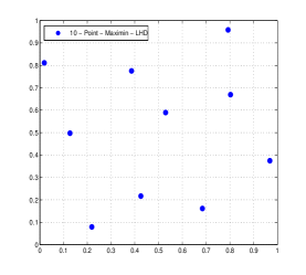
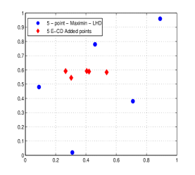
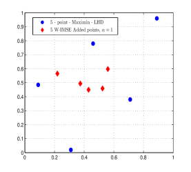
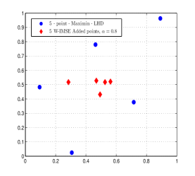
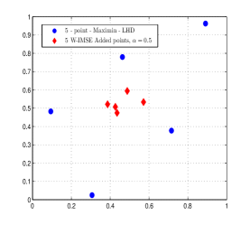
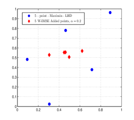
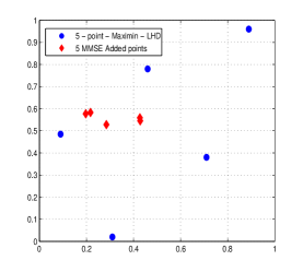
Figure 1: Standard maximin-LHD, ECD design, WIMSE designs of experiments with $\alpha=1,0.8,0.5,0.2$ and MMSE design (two-dimensional toy example).

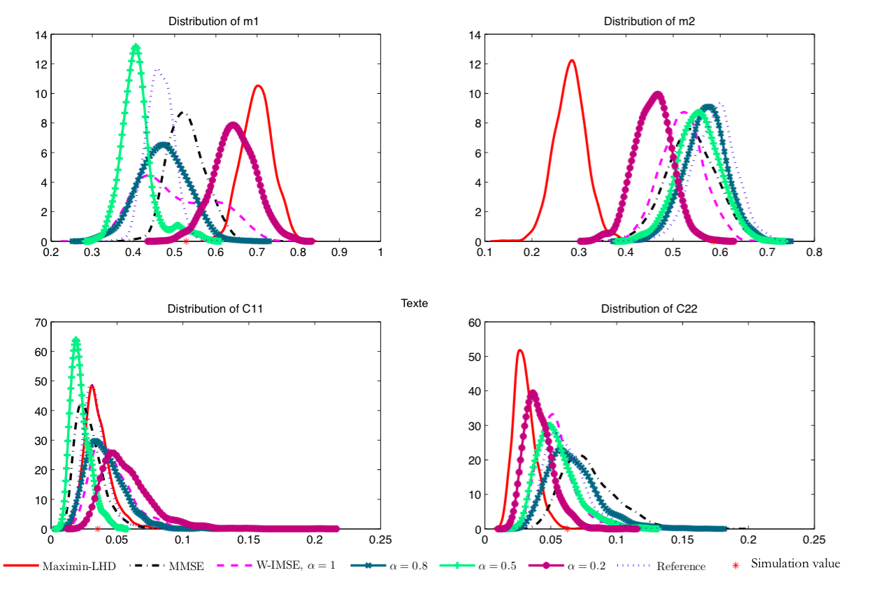
Figure 2: Posterior distributions of $\theta$ with benchmark, standard maximin-LHD, MMSE design and WIMSE designs with $\alpha=1,0.8,0.5,0.2$ (two-dimensional toy example).

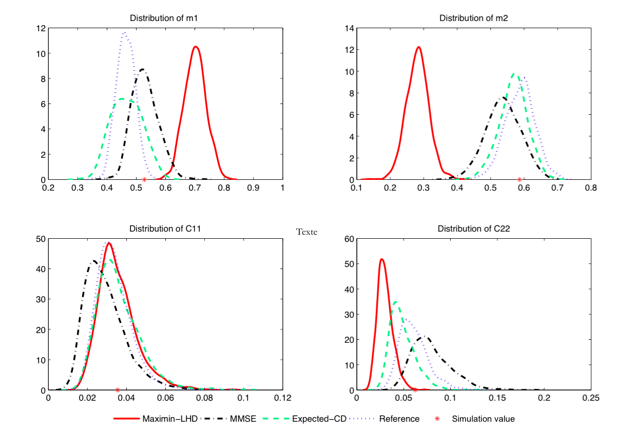
Figure 3: Posterior distributions of $\theta$ with benchmark, standard maximin-LHD, MMSE design and ECD design (two-dimensional toy example).

Figure 1 provides a comparison of all designs with the standard 10-points-maximin-LHD (encompassing the initial DoE). For the W-IMSE criterion, the added points are found not far from the hypothesized mean $(0.5,0.7)$ and the four WIMSE designs are quite similar. However, the posterior distributions of $\theta$ are quite sensitive to the choice of $\alpha$. Figure 2 displays these posterior distributions for the corresponding metamodels. The WIMSE criterion improved the posterior distributions of $m_{2}$ and $C_{22}$, but the choices $\alpha=1,0.5$ and $0.2$ do not work well for the posterior distribution of $m_{1}$ and $C_{11}$. It can be seen that the 10-points-maximin-LHD performs poorly, with respect to a 5-points-maximin-LHD sequentially completed. Moreover, the MMSE criterion performs correctly. However, other experiments, conducted using the best value $\alpha=0.8$ for the WIMSE criterion, are summarized on Figure 3. These results highlight, on this example, that the design build using the ECD criterion can significantly outperform the 10-point-maximin-LHD, can perform more efficiently than the MMSE criterion and can do as well as the WIMSE criterion.

7 Case-study: calibrating roughness coefficients of an hydraulic engineering model

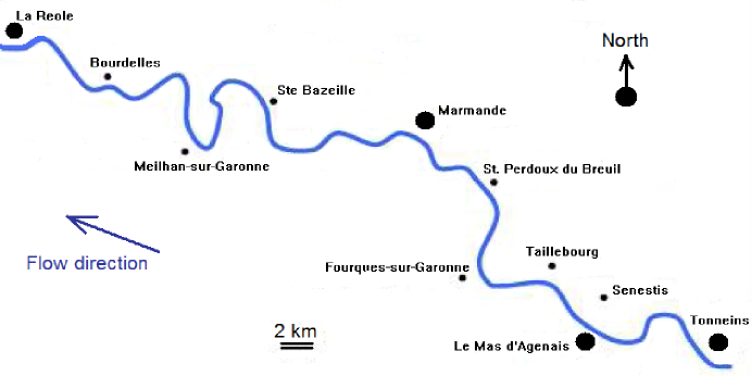
Figure 4: Riverbed profile of French river La Garonne.

The case-study that motivated this work is the calibration, from observed water levels $Y$ and upstream flow values $d$, of the roughness (so-called Strickler) coefficient $X$ of the hydraulic computer model TELEMAC-2D. This software tool is considered as one of the major standards in the field of free-surface flow by solving shallow water (Saint-Venant) equations [14]. This parameter vector summarizes the influence of the land nature on the water level, for a given discharge $d$. The model is used here to reproduce in two dimensions (geographical coordinates) the downstream water level of the French river La Garonne between Tonneins and La Réole (Figure 4).

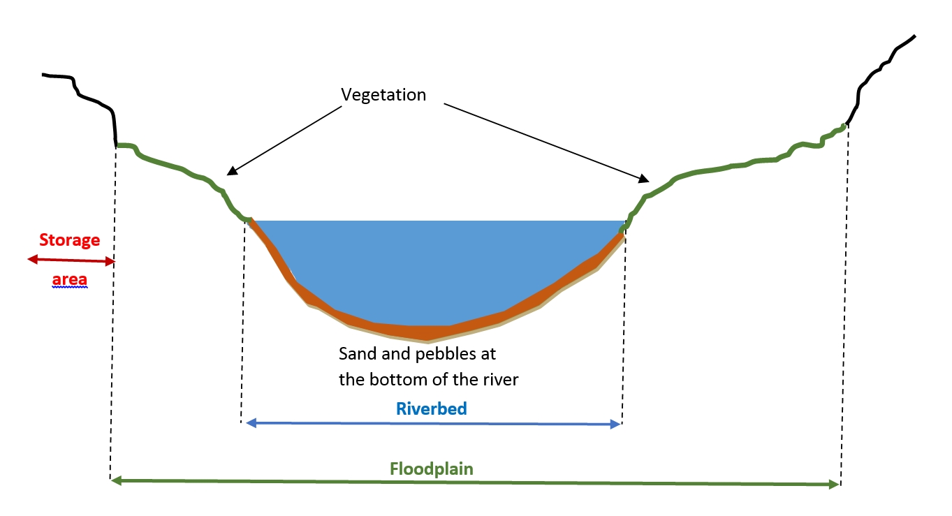
Figure 5: Cross-section of a classical river.

The flow simulation of this 50km river section, including riverbed and floodplain (cf. Figure 5), is conducted on very fine meshes defined by 41,000 knots, each parametrized by a roughness value. The dimension of $X$ is diminished to $q=4$ by taking account of: (a) the homogeneity of the land regularity in large areas surrounding the riverbed between four measuring stations (Table 4 and Figure 4) ; and : (b) the lack of observations of floodplain water levels at the uppermost subsection, which requires to fix the corresponding roughness coefficient. Details about the notation and meaning of each component of $X$ are provided in Table 4.

The strong but physically limited uncertainty that penalizes the knowledge of Strickler coefficients is compatible, according to Wohl, [46], with simple and classic statistical distributions as the Gaussian law (numerically truncated in 0). Based on available bibliography summarized in Table 3 and after discussing with ground experts, values for the hyperparameter $\mu$ for each dimension of $X$ were simple to elicit (see Table 4). It was more tricky to find information about the correlations between the $X$. The strong differences of land nature between the riverbed and the foodplain made plausible the assumption of independence between the corresponding components of $X$. On the contrary, it is likely that two connected riverbed section share roughness features. However, in absence of any additional information about these possibe correlations, $C_{e}$ was chosen diagonal:

$$C_{e} = \left(\begin{array}[]{llll}\sigma^{2}_{\text{maj}}&0&0&0\\ 0&\sigma^{2}_{\text{min}_{TA}}&0&0\\ 0&&\sigma^{2}_{\text{min}_{AA}}&\\ 0&0&0&\sigma^{2}_{\text{min}_{AL}}\\ \end{array}\right).$$

The calibration of each $\sigma$ was conducted by using marginal prior knowledge about the mean variation of the Manning coefficient $M=1/X$, discussed in Liu, [22] and displayed on Figure 6. A prior Manning estimator $(\hat{M}=1/\mu,\sigma_{M})$ can then be produced. A magnitude for the corresponding prior estimator of $\sigma$ (for the Strickler $X=1/M$) can be derived assuming that the results on Table 3 and Figure 6 summarize a large number of past estimations. Further to this assumption, a crude in-law convergence

$$\sigma^{-1}_{M}(\hat{M}-M) \xrightarrow{{\cal{L}}}{} {\cal{N}}(0,1).$$

associated to a Delta method provides the approximate result

$$\mu^{-2}\sigma^{-1}_{M}(\mu-X) \xrightarrow{{\cal{L}}}{} {\cal{N}}(0,1),$$

and finally $\sigma^{2}\simeq\mu^{4}\sigma^{2}_{M}$. The prior assessments of these variances are provided on Table 3, assuming a virtual size $a=1$ for each dimension (see $\S$ 3.1 for details).

The relevance of a metamodelling approach was acknowledged since each run of TELEMAC-2D can take several hours. Maximin-LHD designs were produced over the domain $\Omega$, defined for the input vector $z=(x,d)$ as

$$\Omega = \Omega_{\text{maj}}\times\Omega_{\text{min}_{TA}}\times\Omega_{\text{min}_{AA}}\times\Omega_{\text{min}_{AL}}\times\Omega_{d}$$

in function of the bounds of variation domains summarized in Table 3: $\Omega_{\text{maj}}=[0,30]$ and $\Omega_{\text{min}_{TA}}=\Omega_{\text{min}_{AA}}=\Omega_{\text{min}_{AL}}=[20,70]$ (in $(m^{1/3}.s^{-1})$). The domain $\Omega_{d}$ was chosen as $[q_{0.05},q_{0.95}]=[510,2373]$ where $q_{\alpha}$ is the $\alpha-$order percentile of the known flow distribution, which is Gumbel with mode 1013 $m^{3}.s^{-1}$ and scale parameter 458.

Before running TELEMAC-2D, however, a Bayesian inferential study was briefly conducted using the MASCARET simplified computer code [15], which describes a river by a curvilinear abscissa and uses the same input vector. While much more imprecise than TELEMAC-2D, the advantage of this simplified model is that the CPU time used for one run is shorter, so that the MCMC proposed in [13] can be conducted in due time using a static Maximin-LHD design (and metamodelling calibrated once), using 20,000 iterations. The aim of this study was to test the agreement between the prior assessments and the observations, following recommendations in [7, 13]. A set of $n=50$ observations were available, among which the 10 most recent were preferentially selected, as the most representative of the actual conditions (riverbed homogeneity). For several sizes of design and the two datasets the marginal posterior distributions are displayed on Figure 7. For each dimension, it appears that the regions of highest posterior density are in accordance with the prior guesses, which makes us confident in the relevance of the prior elicitation process.

Based on this good relevance of the Bayesian model, a comparison of the three designs considered in this article was conducted by comparing the emulator errors yielded by the designs, using the coefficient of predictability $Q_{2}$. A cross-validation leave-one-out version of this criterion is used here for computational simplicity [40]:

$$Q_{2} = 1-\frac{\mbox{PRESS}}{\sum_{i=1}^{N}\big{\|}H(z_{(i)})-\overline{H}_{D_{N}}\big{\|}^{2}}.$$

where $\overline{H}_{D_{N}}=\frac{1}{N}\sum_{i=1}^{N}H(z_{(i)})$ and $\mbox{PRESS}=\sum_{i=1}^{N}e_{(i)}^{2}\,=\,\sum_{i=1}^{N}\big{\|}H(z_{(i)})-\widehat{H}_{-i}(z_{(i)})\big{\|}^{2}$, with

• $e_{(i)}$ is the prediction error at $z_{(i)}$ of a fitted model without the point $z_{(i)}$;

• $\widehat{H}_{-i}(z_{(i)})$ is the approximation of $H$ at $z_{(i)}$ derived from all the points of the design except $z_{(i)}$.

The closer $Q_{2}$ to 1, the smaller the variance explained by the emulator and the better the quality of the design (in terms of prediction power for the metamodel). Four designs are tested. Two Maximin-LHD designs $D_{20}$ and $D_{500}$ of 20 and 500 points, respectively (the second one playing the role of a ”reference design” leading to a very good approximation of the posterior distribution. Two other designs are sequentially elaborated using the ECD and WISE criterion, starting from an initial design $D_{10}$ of 10 points: 10 other points are added.

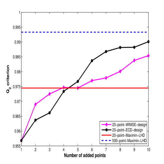
Figure 8: Comparison of the quality of different designs of numerical experiments using the MASCARET computer code.

Displayed on Figure 8, the $Q_{2}$ coefficient related to the maximin-LHD $D_{20}$ equals 0.9745 and the benchmark $Q_{2}$ corresponding to the $D_{500}$ equals 0.9933. Starting from a design of 10 points only, it appears natural that other designs are characterized by a lower $Q_{2}$. However, by adding 10 points iteratively to the initial design $D_{10}$ according to the two proposed criteria, an increasing value of $Q_{2}$ is obtained, which quickly beats the predictability generated by the maximin-LHD $D_{20}$. Finally using the ECD criterion provides a slightly better $Q_{2}$ value than using the WISE criterion.

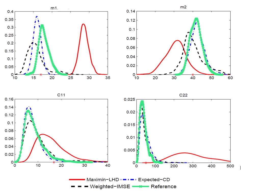
Figure 9: Approximations of the marginal posterior distributions of $\theta$ (first four dimensions) produced by several designs using the TELEMAC-2D computer code. The red stars indicates the prior means for each parameter.

Coming back to the TELEMAC-2D computer code, the convergence of MCMC chains were obtained (using the $n=10$ best observations) after 30,000 iterations. For the various designs proposed in this article, the marginal posterior distributions of the four first parameters are displayed on Figure 9. The Maximin-LHD design $D_{20}$ (producing the approximate posterior in red) was made of 40 points, while other situations start from a DOE of 20 initial points, to which 20 other points are added sequentially (producing the approximate posteriors in blue and black). The reference Maximin-LHD design $D_{500}$ (producing the best approximation of the target posterior, in green) is made of 500 points, as for the MASCARET application. A better proximity of the approximate posterior distribution produced using ECD to the target can be again noticed with respect to the approximation produced by the WIMSE approach.

8 Conclusions and perspectives

This article aims to provide an adaptive methodology to calibrate, in a Bayesian framework, the distribution of unknown inputs of a nonlinear, time-consuming numerical model from observed outputs. This methodology is based on improving a space-filling design of experiments, typically the maximin-Latin Hypercube Design, that offers a non-intrusive exploration of the model. Kriging metamodelling is used to avoid costly runs of the model.

In this methodology, two adaptive criteria have been proposed to complete sequentially the current design. The first one is an adaptation of the standard Weighted-IMSE criterion to the Bayesian framework. It is obtained by weighting the MSE term over a region of interest indicated by the current full conditional posterior distribution. The other criterion, called Expected CD, is based on maximizing the Kullback-Leibler (KL) divergence between two consecutive approximate posterior distributions related to the DoE. A clearer interpretation can be given to the second criterion, as a crude approximation of the negative KL divergence between the target posterior and the current approximate posterior distributions.

Numerical experiments have highlighted, on two examples, that applying this adaptive procedure can reduce the prediction error and improve the accuracy of the metamodeling approximation, compared with a standard space-filling DoE. Therefore such adaptive procedures appear to be useful when the CPU time required to compute an occurrence of the simulator $H$ of physical models is dramatically greater than the time required to run a Gibbs sampler, a Monte Carlo integration or to perform an optimization with a Simulated Annealing procedure.

Both criteria involve expensive numerical integration. For a similar gain in information, the ECD criterion appears to be a little more expensive than the WIMSE criterion since it requires the calculation of the empirical KL divergence. However, in the definition of WIMSE, the choice of $\alpha$ is quite important. As the second weight function is globally much smaller that the first prediction error, this balance parameter permits us to find a good behavior of this criterion. In this article, this important parameter was not systematically studied, but the computation of the best (or at least a ”good”) value of $\alpha$ makes the use of WIMSE much less easy. In addition of this better interpretation (in information-theoretic terms), this feature lets us have a clear preference for the use of the ECD criterion.

This work is a first approach to designing sequential strategies for both exploring a black-box, time-consuming computer code and in parallel calibrating some of its unobserved random inputs. The democratized use of metamodelling requires, in practice, to make various approximations. For instance, it is current that the hyper-parameters of kriging metamodels are updated (e.g., by maximum likelihood estimation) after several additions of points to an original design, since each updating (which should be formally conducted after each addition of a new point) can be a costly operation itself without fundamental improvement [38, 39]. Following a same idea of reaching a trade-off between a theoretical aim and practical easiness, idealistic criteria are often necessarily approximated, or favored partially because their computation can made explicit. This is for instance the case of the Expected Improvement (EI) criterion proposed by Jones et al., [17] which makes profit from the Gaussian properties of kriging metamodels.

Such approximations appeared needed to conduct this first study and highlight the interest of the approach. The rationale developed in Section 4 must now be followed by a truly theoretical work that could robustify the proposed choices, accompanied with more systematical simulation studies with other static or dynamic designs of numerical experiments. Especially, the statistical control of the metamodelling-based posterior approximation with respect to the target posterior should be a focus point in future studies, by making profit of the relationships between Kullback-Leibler divergences and discrepancy measures [29] as well as recent theoretical developments about relaxing assumptions under which metamodelling provides a fair approximation of the real numerical model (e.g., Vazquez and Bect, [42]). Such works are currently being conducted. For the present time, it must be noticed that the approximate posterior distribution produced by the ECD approach can be considered as a fast non-intrusive way of modelling an instrumental distribution, to be used in a final step of importance sampling (typically to compute a posterior mean), provided a small computational budget be kept or made available for running the numerical model.

Appendix A. Metropolis-Hastings step within the Gibbs sampler

At step $r+1$ of Gibbs sampling, after simulating $m^{(r+1)}$,$C^{(r+1)}$, the missing data $\mathbf{X}^{(r+1)}$ can be updated with a Metropolis-Hasting (MH) algorithm. The MH step is updating $\mathbf{X}^{(r)}=(X^{r}_{1},\dots,X^{r}_{n})^{\prime}$ in the following way:

• For $i=1,\ldots,n$

  1. Generate $\widetilde{X}_{i}\sim J(\cdot\mid X_{i}^{r})$ where $J$ is the proposal distribution.

  2. Let

     $$\alpha(X_{i}^{r},\widetilde{X}_{i}) = \min\Big{(}\frac{\pi_{\widehat{H}}(\widetilde{\mathbf{X}}\mid\boldsymbol{\mathcal{Y}},\theta^{(r+1)},\rho,\mathbf{d},H_{D})\,J(X_{i}^{r}|\widetilde{X}_{i})}{\pi_{\widehat{H}}(\mathbf{X}^{(r)}\mid\boldsymbol{\mathcal{Y}},\theta^{(r+1)},\rho,\mathbf{d},H_{D})\,J(\widetilde{X}_{i}|X_{i}^{r})},1\Big{)},$$

     where

     $$\widetilde{\mathbf{X}} = \Big{(}X_{1}^{r+1},\,\dots,\,X_{i-1}^{r+1},\,\widetilde{X}_{i},\,X_{i+1}^{r},\,\dots,\,X_{n}^{r}\Big{)}^{\prime}$$

     $$\mathbf{X}^{(r)} = \Big{(}X_{1}^{r},\,\dots,\,X_{i-1}^{r},\,X_{i}^{r},\,X_{i+1}^{r},\,\dots,\,X_{n}^{r}\Big{)}^{\prime}$$

  3. Take

     $$X_{i}^{r+1} = \left\{\begin{array}[]{ll}\widetilde{X}_{i}&\textrm{{with probability} $\alpha(X_{i}^{r},\widetilde{X}_{i})$},\\ X_{i}^{r+1}&\textrm{{otherwise.}}\end{array}\right.$$

Remarks

• Many choices are possible for the proposal distribution $J$. It appears that choosing an independent MH sampler with $J$ chosen to be the normal distribution $\mathcal{N}\Big{(}m^{(r+1)},C^{(r+1)}\Big{)}$ give satisfying results for the model (1).

• In practice, it can be beneficial to choose the order of the updates by a random permutation of $\{1,\ldots,n\}$ to accelerate the convergence of the Markov chain to its limit distribution.

Appendix B. Nearest-Neighbor approach

The Kullback-Leibler (KL) divergence between samples $\Theta^{i}$ and $\Psi$ can be empirically calculated through the Nearest-Neighbor approach.

$$\widehat{\mbox{KL}}_{L_{1},L_{2}}(\Theta^{i}\,||\,\Psi) = \frac{d}{L_{1}}\sum_{j=1}^{L_{1}}\log\frac{\nu_{L_{2}}(\theta^{i}_{j})}{\rho^{i}_{L_{1}}(\theta^{i}_{j})}\,+\,\log\frac{L_{2}}{L_{1}-1},$$ (42)

where $d$ denotes the dimension of the parameter $\theta$ ($2q$ in our case), $\nu_{L_{2}}(\theta^{i}_{j})$ denotes the (Euclidean) distance between $\theta^{i}_{j}\in\Theta^{i}$ and its nearest neighbor in sample $\Psi$

$$\nu_{L_{2}}(\theta^{i}_{j}) = \min_{\begin{subarray}{c}r=1,\dots,L_{2}\end{subarray}}\,||\theta_{r}-\theta^{i}_{j}||_{2},$$

and $\rho^{i}_{L_{1}}(\theta^{i}_{j})$ denotes the (Euclidean) distance of $\theta^{i}_{j}$ to its nearest neighbor in $\Theta^{i}$ except itself (as it is also included in $\Theta^{i}$)

$$\rho^{i}_{L_{1}}(\theta^{i}_{j}) = \min_{\begin{subarray}{c}l=1,\dots,L_{1};\,l\neq j\end{subarray}}\,||\theta^{i}_{l}-\theta^{i}_{j}||_{2}.$$

It has been proved in [45] that under some regularity conditions on the samples $\Theta^{i}$ and $\Psi$, the estimator $\widehat{\mbox{KL}}_{L_{1},L_{2}}(\Theta^{i}\,||\,\Psi)$ is consistent in the sense that

$$\lim_{L_{1},L_{2}\rightarrow\infty}\mathbb{E}\left(\widehat{\mbox{KL}}_{L_{1},L_{2}}(\Theta^{i}\,||\,\Psi)-\mbox{KL}(\Theta^{i}\,||\,\Psi)\right)^{2} = 0,$$ (43)

and asymptotically unbiased, i.e.

$$\lim_{\begin{subarray}{c}L,R\rightarrow\infty\end{subarray}}\mathbb{E}\left[\widehat{\mbox{KL}}_{L_{1},L_{2}}(\Theta^{i}\,||\,\Psi)\right] = \mbox{KL}(\Theta^{i}\,||\,\Psi).$$ (44)

Appendix C. Simulated Annealing algorithm (searching for the minimum of a function $f$)

Proposed by Kirkpatrick et al., [19], the SA algorithm is a stochastic optimization algorithm.

Given the current point $z^{(k)}$, at iteration $k+1$ :

1. Generate $\widetilde{z}\sim\mathcal{N}\Big{(}z^{(k)},\sigma^{2}\Big{)}$, with a certain fixed variance $\sigma^{2}$.

2. Let

   $$\lambda\Big{(}z^{(k)},\widetilde{z}\Big{)} = \min\Big{(}1,\exp\Big{(}\frac{f(z^{(k)})-f(\widetilde{z})}{\beta_{k+1}}\Big{)}\Big{)},$$

   where $\beta_{k+1}$ is the current temperature at step $k+1$.

3. Accept

   $$z^{[k+1]} = \left\{\begin{array}[]{ll}\widetilde{z},&\textrm{{with probability} $\lambda\Big{(}z^{(k)},\widetilde{z}\Big{)}$},\\ z^{(k)},&\textrm{{otherwise.}}\end{array}\right.$$

4. Update $\beta_{k+1}=0.99\times\beta_{k}$.

DoE 1	10-point-maximin-LHD
DoE 2	5-points-maximin-LHD +	5-points-WIMSE
		or 5-points-ECD
		or 5-points-MMSE
DoE 3	100-points-maximin-LHD (benchmark)

Table 1: Description of the three types of designs of experiments (DOE) (two-dimensional toy example).

WIMSE	$\alpha$	Number $L$ of iterations	Size $M$ of the
		of the SA algorithm	Monte Carlo algorithm
	1, 0.8, 0.5, 0.2	1,000	1,000
ECD	Number $M$ of	Sizes $L_{1}$ and $L_{2}$ of	Number $L$ of iterations
	generated GPs	the samples $\Theta^{i}$ and $\Psi$	of the SA algorithm
	100	1,000	1,000
SA algorithm	Initial point $x^{[0]}$	Initial temperature $\beta$	Standard deviation $\sigma$
	$x$	100	100

Table 2: Choice of parameters for the design criteria computation and the SA algorithm (two-dimensional toy example).

Nature of surface	Value of Strickler coefficient ($m^{1/3}\cdot s^{-1}$)
Riverbed
Smooth concrete	75-90
Earthen channel	50-60
Plain river, without shrub vegetation	35-40
Plain river, with shrub vegetation	30
Slow winding natural river	30-50
Very cluttered riverbed	10-30
Proliferating algae	3.3-12.5
Foodplain
Meadows, uncultivated fields	20
Cultivated lands with low size vegetation	15-20 - 18
Cultivated lands with large size vegetation	10-15 - 13
Bush and undergrowth areas	8-12 - 10
Forest	$<$10
Low density urban sprawl	8-10
High density urban sprawl	5-8

Table 3: Realistic ranges of value for the Strickler coefficient in function of the nature of the surface, summarized from Survey, [36], Walesh, [44], Sellin et al., [33] and Viollet et al., [43]. Median values in bold type are interpreted by international experts as the most likely values taking account of uncertainties about the nature of vegetation, topographic irregularities, etc.

(Sub)section	Position	$X$ component	Marginal hyperparameters $(m^{1/3}.s^{-1})$
Tonneins
$\downarrow$	foodplain	$X_{s,\text{maj}}$	$\mu_{\text{maj}}=17$	$\sigma_{\text{maj}}=4.1$
La Réole
Tonneins
$\downarrow$	riverbed	$X_{s,\text{min}_{TA}}$	$\mu_{\text{min}_{TA}}=45$	$\sigma_{\text{min}_{TA}}=7.1$
Aval de Mas d’Augenais
$\downarrow$	riverbed	$X_{s,\text{min}_{AA}}$	$\mu_{\text{min}_{AA}}=38$	$\sigma_{\text{min}_{AA}}=7.1$
Amont de Marmande
$\downarrow$	riverbed	$X_{s,\text{min}_{AL}}$	$\mu_{\text{min}_{AL}}=40$	$\sigma_{\text{min}_{AL}}=7.1$
La Réole

Table 4: Detailed meanings and prior modelling for each component of $X$ (La Garonne roughness coefficients). The riverbed roughness coefficients are differentiated between the measuring stations listed in the first column. A virtual size $a=1$ was chosen for each dimension.

Figure 7: Approximations of the marginal posterior distributions of $\theta$ for several sizes $N$ maximin-LHD and two encompassed observation datasets ($n=10$ then $n=50$) using the MASCARET computer code.

References

- Bachoc, [2013] Bachoc, F. (2013). Cross validation and maximum likelihood estimation of hyper-parameters of gaussian processes with model misspecification. Computational Statistics and Data Analysis, 66:55–69.
- Barbillon et al., [2011] Barbillon, P., Celeux, G., Grimaud, A., Lefebvre, Y., and tienne de Rocquigny (2011). Nonlinear methods for inverse statistical problems. Computational Statistics & Data Analysis, 55(1):132 – 142.
- Bastos and O’Hagan, [2009] Bastos, L. S. and O’Hagan, A. (2009). Diagnostics for Gaussian process emulators. Technometrics, 51(4):425–438.
- Bayarri et al., [2007] Bayarri, M. J., Berger, J. O., Paulo, R., Sacks, J., Cafeo, J. A., Cavendish, J., Lin, C.-H., and Tu, J. (2007). A framework for validation of computer models. Technometrics, 49(2):138–154.
- Bect et al., [2012] Bect, J., Ginsbourger, D., Li, L., Picheny, V., and Vazquez, E. (2012). Sequential design of computer experiments for the estimation of a probability of failure. Statistics and Computing, 22(3):773–793.
- Berger et al., [2015] Berger, J., Bernardo, J., and Sun, D. (2015). Overall objective priors. Bayesian Analysis, 10:189–221.
- Bousquet, [2008] Bousquet, N. (2008). Diagnostics of prior-data agreement in applied bayesian analysis. Journal of Applied Statistics, 35:1011–1029.
- Bousquet et al., [2015] Bousquet, N., Fouladirad, M., Grall, A., and Paroissin, C. (2015). Bayesian gamma processes for optimizing condition-based maintenance under uncertainty. Applied Stochastic Models in Business and Industry, 31(3):360–379.
- Brooks and Gelman, [1998] Brooks, S. P. and Gelman, A. (1998). General methods for monitoring convergence of iterative simulations. Journal of Computational and Graphical Statistics, 7(4):pp. 434–455.
- Celeux and Diebolt, [1988] Celeux, G. and Diebolt, J. (1988). A random imputation principle: the stochastic em algorithm. Technical Report RR-0901, INRIA.
- Celeux et al., [2010] Celeux, G., Grimaud, A., Lefèbvre, Y., and de Rocquigny, É. (2010). Identifying intrinsic variability in multivariate systems through linearized inverse methods. Inverse Problems in Science and Engineering, 18(3):401–415.
- Cover and Thomas, [2006] Cover, T. M. and Thomas, J. A. (2006). Elements of Information Theory. Wiley-Interscience, 2nd edition edition.
- Fu et al., [2014] Fu, S., Celeux, G., Bousquet, N., and Couplet, M. (2014). Bayesian inference for inverse problems occurring in uncertainty analysis. International Journal for Uncertainty Quantification. Forthcoming article.
- Galland et al., [1991] Galland, J., Goutal, N., and Hervouet, J. (1991). Telemac: A new numerical model for solving shallow water equations. Advances in Water Resources, 14(3):138–148.
- Goutal et al., [2012] Goutal, N., Lacombe, J.-M., Zaoui, F., and El-Kadi-Abderrezzak, K. (2012). Mascaret: a 1-d open-source software for flow hydrodynamic and water quality in open channel networks. River Flow, pages 1169–1174.
- Johnson et al., [1990] Johnson, M. E., Moore, L. M., and Ylvisaker, D. (1990). Minimax and maximin distance design. Journal of Statistical Planning and Inference, 26(2):131–148.
- Jones et al., [1998] Jones, D. R., Schonlau, M., and Welch, W. J. (1998). Efficient global optimization of expensive black-box functions. Journal of Global Optimization, 13:455–492.
- Kennedy and O’Hagan, [2001] Kennedy, M. C. and O’Hagan, A. (2001). Bayesian calibration of computer models. Journal of the Royal Statistical Society: Series B (Statistical Methodology), 63(3):425–464.
- Kirkpatrick et al., [1983] Kirkpatrick, S., Gelatt, C. D., and Vecchi, M. P. (1983). Optimization by simulated annealing. Science, 220(4598):671–680.
- Koehler and Owen, [1996] Koehler, J. and Owen, A. (1996). Computer experiments. In Ghosh, S. and Rao, C., editors, Design and analysis of experiments, volume 13 of Handbook of statistics, pages 261–308. Elsevier.
- Liu and Rubin, [1994] Liu, C. and Rubin, D. B. (1994). The ecme algorithm: A simple extension of em and ecm with faster monotone convergence. Biometrika, 81(4):633–648.
- Liu, [2009] Liu, D. (2009). Uncertainty Quantification with Shallow Water Equations. PhD thesis, Ph. Dissertation in Natural Risk Management, Carl-Friedrich-Gauss Faculty, University of Braunschweig.
- Matheron, [1971] Matheron, G. (1971). The theory of regionalized variables and its applications. Les Cahiers du Centre de Morphologie Mathématique de Fontainebleau, Fascicule 5. École des Mines de Paris.
- McKay et al., [1979] McKay, M. D., Beckman, R. J., and Conover, W. J. (1979). A comparison of three methods for selecting values of input variables in the analysis of output from a computer code. Technometrics, 21:239–245.
- Mockus et al., [1978] Mockus, J., Tiesis, V., and Zilinskas, A. (1978). The application of bayesian methods for seeking the extremum. In Dixon, L. and Szego, G., editors, Global Optimization, volume 2, pages 117–129. North Holland, New York.
- Morris and Mitchell, [1995] Morris, M. and Mitchell, T. (1995). Exploratory designs for computationnal experiments. Journal of Statistical Planning and Inference, 43:381–402.
- of Engineers, [1996] of Engineers, U. A. C. (1996). Risk-analysis for flood damage reduction studies. Technical Report No. EM 1110-2-1619.
- Picheny et al., [2010] Picheny, V., Ginsbourger, D., Roustant, O., Hafka, R., and Kim, N.-H. (2010). Adaptive designs of experiments for accurate approximation of a target region. Journal of Mechanical Design, 132(7).
- Pollard, [2013] Pollard, D. (2013). Asymptotia: An Exposition of Statistical Asymptotic Theory. On line books.
- Rasmussen and Williams, [2006] Rasmussen, C. E. and Williams, C. K. I. (2006). Gaussian Processes for Machine Learning. MIT Press. ISBN-13 978-0-262-18253-9.
- Sacks et al., [1989] Sacks, J., Welch, W., Mitchell, T., and Wynn, H. (1989). Design and analysis of computer experiments. Statistical Science, 4(4):409–435.
- Santner et al., [2003] Santner, T. J., Williams, B. J., and Notz, W. I. (2003). The design and analysis of computer experiments. Springer Series in Statistics. Springer.
- Sellin et al., [1997] Sellin, R., Keast, J., and Beeston, D. V. (1997). Seasonal variation in river channel hydraulic roughness. In Proceedings of the 27 IAHR World Congress ”Water for a Changing Global Community” - Theme B: Environmental and Coastal Hydraulics: Protecting the Aquatic Habitat, pages 1390–1396.
- Stein, [1964] Stein, C. (1964). Inadmissibility of the usual estimator for the variance of a normal distribution with unknown means. Annals of the Institute of Mathematical Statistics, 16:155–160.
- Stein, [1999] Stein, M. L. (1999). Interpolation of Spatial Data - Some Theory for Kriging. Springer Series in Statistics. Springer-Verlag New York.
- Survey, [1989] Survey, U. G. (1989). Guide for selecting Manning’s roughness coefficients for natural channels and flood plains. U.S. Geologogical Survey Water Supply, paper 2339.
- Tierney, [1996] Tierney, L. (1996). Introduction to general state-space markov chain theory. In Gilks, W. R., Richardson, S., and Spiegelhalter, D. J., editors, Markov Chain Monte Carlo in Practice, Interdisciplinary Statistics, chapter 4, pages 59–74. Chapman & Hall/CRC.
- Toal et al., [2008] Toal, D. J., Bressloff, N. W., and Keane, A. J. (2008). Kriging hyperparameter tuning strategies. The American Institute of Aeronautics and Astronautics (AIAA) Journal, 46:1240–1252.
- Toal et al., [2011] Toal, D. J., Bressloff, N. W., Keane, A. J., and Holden, C. (2011). The development of a hybridized particle swarm for kriging hyperparameter tuning. Engineering Optimization, 43:1–28.
- Vanderpoorten and Palm, [2001] Vanderpoorten, A. and Palm, R. (2001). Compared regression methods for inferring ammonium nitrogen concentrations in running freshwaters from aquatic bryophyte assemblages. Hydrobiologia, 452(1-3):181–190.
- Vazquez and Bect, [2009] Vazquez, E. and Bect, J. (2009). A sequential bayesian algorithm to estimate a probability of failure. In 15th IFAC Symposium on System Identification.
- Vazquez and Bect, [2011] Vazquez, E. and Bect, J. (2011). Sequential search based on kriging: convergence analysis of some algorithms. ISI ? 58th World Statistics Congress of the International Statistical Institute (ISI?11), Dublin, Ireland, August 21-26:1.
- Viollet et al., [1998] Viollet, P.-L., Chabard, J.-P., Esposito, P., and Laurence, D. (1998). Mécanique des Fluides Appliquée. Presses de l’École Nationale des Ponts et Chaussées.
- Walesh, [1989] Walesh, S. (1989). Urban Water Surface Management. John Wiley and Sons.
- Wang et al., [2009] Wang, Q., Kulkarni, S. R., and Verdú, S. (2009). Divergence estimation for multidimensional densities via k-nearest-neighbor distances. IEEE Transactions on Information Theory, 55(5):2392–2405.
- Wohl, [1998] Wohl, E. (1998). Uncertainty in flood estimates associated with roughness coefficient. Journal of Hydraulic Engineering, 124(2):219–223.