On the de Sitter Tardyons and Tachyons

Abstract

It is shown that on the de Sitter manifolds the tachyonic geodesics are restricted such that the classical tachyons cannot exist on this manifold at any time. On the contrary, the theory of the scalar quantum tachyons is free of any restriction. The tachyonic scalar and Dirac plane waves are deduced in this geometry, pointing out that these are well-defined, behaving as tempered distributions at any moment.

Pacs: 04.62.+v

Keywords: de Sitter; classical tachyons; scalar tachyons; Dirac tachyons.

1 Introduction

In special relativity one knows three types of particles, tardyons (subluminal), light-like and tachyons (superluminal). The first two types of particles are of our world, inside the light-cone, while the tachyons seems to live in another one, outside the light-cone. These two worlds seems to be completely separated as long as there are no direct physical evidences about the tardyon-tachyon interactions. For this reason the tachyons are the most attractive hypothetical objects for speculating in some domain in physics where we have serious difficulties in building coherent theories. We mention, as an example, the presumed role of the tachyons in the early brane cosmology [1]. However, here we do not intend to comment on this topics, restricting ourselves to analyze, from the mathematical point of view, the possibility to meet classical or quantum scalar or Dirac tachyons on the de Sitter backgrounds.

The de Sitter manifold, denoted from now by $M$, is local-Minkowskian such that the tachyons can be defined as in special relativity, with the difference that their properties are arising now from the specific high symmetry of the de Sitter manifolds. It is known that the isometry group of $M$, denoted by $I(M)=SO(1,4)$, is in fact the gauge group of the Minkowskian five-dimensional manifold $M^{5}$ embedding $M$. The unitary irreducible representations of the corresponding group $S(M)={\rm Spin}(1,4)=Sp(2,2)$ are well-studied [2] and used in various applications. Many authors exploited this high symmetry for building theories of quantum fields, either by constructing symmetric two-point functions, avoiding thus the canonical quantization [3], or by using directly these unitary representations for finding field equations but without considering covariant representations [4, 5]. Another approach which applies the canonical quantization to the covariant fields transforming according to induced covariant representations was initiated by Nachtmann [6] many years ago and continued in few of our papers [7, 8, 9].

In what follows we would like to study the tachyons on $M$ in this last framework by using the traditional definition of tachyons as particles of real squared masses but of opposite sigs with respect to the tadyonic ones. For this reason our results are different from other approaches [4, 5] where particles whose squared masses are supposed to be complex numbers are considered as tachyon [5]. Thus we find a result that seems to be somewhat paradoxical, namely that the classical tachyons cannot exist on $M$ at any time while the quantum scalar and Dirac particles behaves normally on this manifold, without any restriction.

The paper is organized as follows. In the next section we present the geodesics depending on a parameter giving their types (tardyonic, tachyonic or light-like) and we argue why the tachyonic lifetime is restricted on $M$. The next section is devoted to the quantum scalar and Dirac tachyons whose theory does not meet difficulties such that the mode functions are defined correctly as tempered distributions on the entire space at any moment. Finally, we present the principal conclusion concerning the discrepancy between the classical and quantum cases.

2 Classical de Sitter geodesics

The de Sitter spacetime $M$ is defined as the hyperboloid of radius $1/\omega$ in the five-dimensional flat spacetime $(M^{5},\eta^{5})$ of coordinates $z^{A}$ (labeled by the indices $A,\,B,...=0,1,2,3,4$) and metric $\eta^{5}={\rm diag}(1,-1,-1,-1,-1)$. The local charts $\{x\}$ can be introduced on $(M,g)$ giving the set of functions $z^{A}(x)$ which solve the hyperboloid equation,

$$\eta^{5}_{AB}z^{A}(x)z^{B}(x)=-\frac{1}{\omega^{2}}\,.$$ (1)

Here we use the chart $\{t,\vec{x}\}$ with the conformal time $t$ and Cartesian spaces coordinates $x^{i}$ defined by

$$z^{0}(x) = -\frac{1}{2\omega^{2}t}\left[1-\omega^{2}({t}^{2}-\vec{x}^{2})\right]$$

$$z^{i}(x) = -\frac{1}{\omega t}x^{i}\,,$$ (2)

$$z^{4}(x) = -\frac{1}{2\omega^{2}t}\left[1+\omega^{2}({t}^{2}-\vec{x}^{2})\right]$$

This chart covers the expanding portion, $M_{+}$, of $M$ for $t\in(-\infty,0)$ and $\vec{x}\in{{R}}^{3}$ while the collapsing part, $M_{-}$, is covered by a similar chart but with $t>0$. Both these charts have the conformal flat line element,

$$ds^{2}=\eta^{5}_{AB}dz^{A}(x)dz^{B}(x)=\frac{1}{\omega^{2}{t}^{2}}\left({dt}^{2}-d\vec{x}^{2}\right)\,.$$ (3)

We remind the reader that on each portion one can introduce a FLRW chart with proper time defined as,

$$t_{proper}=\left\{\begin{array}[]{cllll}-\frac{1}{\omega}\ln(-\omega t)&{\rm on}&M_{+}&{\rm for}&-\infty<t<0\,,\\ &&&&\\ \frac{1}{\omega}\ln(\omega t)&{\rm on}&M_{-}&{\rm for}&0<t<\infty\,,\end{array}\right.$$ (4)

such that this spans the whole real axis, $t_{proper}\in(-\infty,\infty)$, on each portion.

By definition, the de Sitter spacetime $M$ is a homogeneous space of the pseudo-orthogonal group $SO(1,4)$ which is in the same time the gauge group of the metric $\eta^{5}$ and the isometry group, $I(M)$, of $M$. The classical conserved quantities as well as the basis-generators of the covariant representations of the isometry group can be calculated with the help of the Killing vectors $k_{(AB)}$ which have the following components:

$$k^{0}_{(0i)}=k^{0}_{(4i)}=\omega tx^{i}\,,\qquad k^{j}_{(0i)}=k^{j}_{(4i)}-\frac{1}{\omega}\,\delta^{j}_{i}=\omega x^{i}x^{j}-\delta^{j}_{i}\chi\,,$$ (5)

$$k^{0}_{(ij)}=0\,,\quad k^{l}_{(ij)}=\delta^{l}_{j}x^{i}-\delta^{l}_{i}x^{j}\,;\qquad k^{0}_{(04)}=t\,,\quad k^{i}_{(04)}=x^{i}\,.$$ (6)

where

$$\chi=\frac{1}{2\omega}\left[1-\omega^{2}(t^{2}-{\vec{x}}^{2})\right]\,.$$ (7)

Furthermore, It is a simple exercise to integrate the geodesic equations and to find the conserved quantities on a geodesic trajectory on $M$. Using the standard notation $u^{\mu}=\frac{dx^{\mu}(s)}{ds}$ we bear in mind that the principal invariant $u^{2}=g_{\mu\nu}u^{\mu}u^{\nu}=\epsilon$ along the geodesics $x=x(s)$ determines the type of this trajectory, i. e. tardyonic ($\epsilon=1$), light-like ($\epsilon=0$) or tachyonic ($\epsilon=-1$). All the other conserved quantities along the geodesics are proportional to $k_{(AB)\,\mu}u^{\mu}$ and can be derived by using the Killing vectors (5) and (6).

We assume first that in the chart $\{t,\vec{x}\}$ the particle of mass $m\not=0$ has the conserved momentum $\vec{p}$ of components $p\,^{i}=\omega m(k_{(0i)\,\mu}-k_{(4i)\,\mu})u^{\mu}$ so that we can write

$$u^{0}=\frac{dt}{ds}=-\omega t\sqrt{\epsilon+\frac{\omega^{2}{p}^{2}}{m^{2}}t^{2}}\,,\qquad u^{i}=\frac{d{x^{i}}}{ds}=(\omega t)^{2}\frac{p\,^{i}}{m}\,,$$ (8)

using the notation $p=|{\vec{p}}\,|$. Hereby we deduce the trajectory,

$${x}^{i}(t)={x}_{0}^{i}+\frac{p\,^{i}}{\omega{p}^{2}}\,\left(\sqrt{\epsilon m^{2}+{p}^{2}\omega^{2}t_{0}^{2}}-\sqrt{\epsilon m^{2}+{p}^{2}\omega^{2}t^{2}}\,\right)\,,$$ (9)

of a massive particle passing through the point $\vec{x}_{0}$ at time $t_{0}$. The light-like case must be treated separately finding that the trajectory of a massless particle reads

$${x}^{i}(t)={x}_{0}^{i}+n^{i}\left(t_{0}-t\right)\,,$$ (10)

where the unit vector $\vec{n}$ gives the propagation direction.

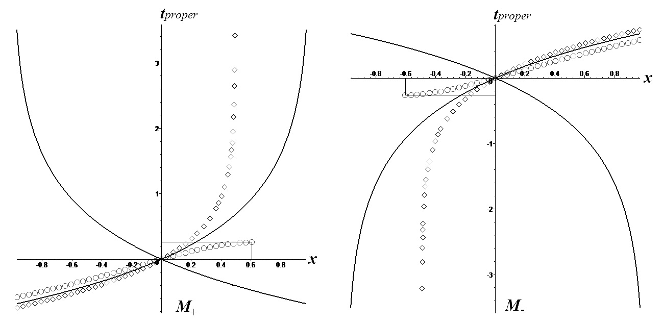
Figure 1: The worldlines of the tardyons (diamonds) and tachyons (circles) with the same momentum and the initial conditions $x_{0}=0$ and either $t_{0}=-\frac{1}{\omega}$ on $M_{+}$ (left panel) or $t_{0}=\frac{1}{\omega}$ on $M_{-}$ (right panel). The solid lines represent the light-cones which tends asymptoticly to the event horizon at $x=\pm\frac{1}{\omega}$.

Among the conserved quantities that can be derived as in Ref. [8] the energy of the massive particles,

$$E=\omega\,\vec{x}_{0}\cdot\vec{p}+\sqrt{\epsilon m^{2}+{p}^{2}\omega^{2}t_{0}^{2}}\,,$$ (11)

indicates the allowed domains of our parameters. Thus we see that the tardyonic particles can have any momentum, $\vec{p}\in{{R}}^{3}_{p}$, since their energies remain always real numbers. When the tardyonic particle is at rest, staying in $\vec{x}(t)=\vec{x}_{0}$ with $\vec{p}=0$, then we find the same rest energy $E_{0}=m$ as in special relativity. Thus we conclude that the tardyonic particles behave familiarly just as in Minkowski flat spacetime.

However, the tachyons have a new and somewhat strange behavior. When $\epsilon=-1$ there are real trajectories only for large momentum with $|\vec{p}|>m$, corresponding to the superluminal motion. Moreover, we must have $p^{2}\omega^{2}t_{0}^{2}\geq m^{2}$ which means that $t_{0}$ satisfies either the condition $t_{0}\leq-\frac{m}{p\omega}$ on $M_{+}$ or the symmetric one $t_{0}\geq\frac{m}{p\omega}$ on $M_{-}$. Thus we conclude that a classical tachyon of momentum $p>m$ can exist on the expanding portion only in the time domain $-\infty<t\leq-\frac{m}{p\omega}$ while on the collapsing portion its time domain is $\frac{m}{p\omega}\leq t<\infty$. The corresponding time domains of the tachyons with momentum $p>m$ in the charts of proper time are now $(-\infty,\frac{1}{\omega}\ln(\frac{p}{m}))$ on $M_{+}$ and $(-\frac{1}{\omega}\ln(\frac{p}{m}),\infty)$ on $M_{-}$. In Fig. (1) we represent the worldlines in terms of the proper time with the initial conditions read $x_{0}=0$ at $t_{0}=\mp\frac{1}{\omega}$ for which $t_{proper}=0$ on both the portions of $M$.

These restrictions upon the tachyonic lifetime are quite unusual opening the problem of finding a plausible mechanism explaining the tachyon death on $M_{+}$ or how this is born on $M_{-}$.

3 Quantum modes

The next step is to verify if similar restrictions could could arise in the case of the quantum fields too. For this purpose we have to analyse the tachyonic solutions of the scalar and Dirac fields in momentum representation.

The specific feature of the quantum mechanics on $M$ is that the energy operator does not commute with the components of the momentum operator. Therefore, the energy and momentum cannot be measured simultaneously with a desired accuracy. Consequently, there are no particular solutions of the Klein-Gordon or Dirac equations with well-determined energy and momentum, being forced to consider different plane waves solutions depending either on momentum or on energy and momentum direction. In what follows we restrict ourselves to the plane waves of determined momentum.

3.1 Scalar plane waves

In an arbitrary chart $\{x\}$ the action of a charged scalar field $\phi$ of mass $m$, minimally coupled with the gravitational field, reads

$${\cal S}[\phi,\phi^{*}]=\int d^{4}x\sqrt{g}\,{\cal L}=\int d^{4}x\sqrt{g}\left(\partial^{\mu}\phi^{*}\partial_{\mu}\phi-\epsilon m^{2}\phi^{*}\phi\right)\,,$$ (12)

where $g=|\det(g_{\mu\nu})|$ and $\epsilon$ is our parameter which gives the tardyonic, tachyonic or light-like behaviour. This action gives rise to the KG equation

$$\frac{1}{\sqrt{g}}\,\partial_{\mu}\left[\sqrt{g}\,g^{\mu\nu}\partial_{\nu}\phi\right]+\epsilon m^{2}\phi=0\,,$$ (13)

whose solutions have to be normalized (in generalized sense) with respect to the relativistic scalar product [10],

$$\langle\phi,\phi^{\prime}\rangle=i\int_{\Sigma}d\sigma^{\mu}\sqrt{g}\,\phi^{*}\stackrel{{\scriptstyle\leftrightarrow}}{{\partial_{\mu}}}\phi^{\prime}\,,$$ (14)

written with the notation $f\stackrel{{\scriptstyle\leftrightarrow}}{{\partial}}h=f(\partial g)-g(\partial f)$.

In the chart $\{t,\vec{x}\}$ we use here the Klein-Gordon equation takes the form,

$$\omega^{2}t^{2}\left(\partial_{t}^{2}-\frac{2}{t}\partial_{t}-\Delta\right)\phi(x)+\epsilon m^{2}\psi(x)=0\,.$$ (15)

The solutions of this equation may be square integrable functions or tempered distributions with respect to the scalar product (14) that for $\Sigma={{R}}^{3}$ takes the form

$$\langle\phi,\phi^{\prime}\rangle=i\int d^{3}x\,e^{3\omega t}\,\phi^{*}(x)\stackrel{{\scriptstyle\leftrightarrow}}{{\partial_{t}}}\phi^{\prime}(x)\,.$$ (16)

It is known that the KG equation (15) of NP can be analytically solved in terms of Bessel functions [10]. There are fundamental solutions of positive frequencies and given momentum, $\vec{p}$, that read

$$f_{\vec{p}}(x)=\frac{1}{2}\sqrt{\frac{\pi}{\omega}}\frac{e^{-\frac{1}{2}i\pi k}}{(2\pi)^{3/2}}\,(-\omega t)^{\frac{3}{2}}H^{(1)}_{k}\left(-pt\right)e^{i\vec{p}\cdot\vec{x}}\,,$$ (17)

where $H^{(1)}_{\nu}$ are Hankel functions, $p=|\vec{p}|$ and we denote

$$k=\sqrt{\frac{9}{4}-\epsilon\frac{m^{2}}{\omega^{2}}}\,.$$ (18)

Obviously, the fundamental solutions of negative frequencies are $f_{\bf p}^{*}(x)$.

Now we observe that the only parameter depending on $\epsilon$ is just that given by Eq. (18) which encapsulates the information about the nature of the scalar particle. We observe first that there are no major differences between the tardyonic ($\epsilon=1$) and tachyonic ($\epsilon=-1$) cases. The only property depending on the particle’s nature is the behavior of the mode functions in the limit of $t\to 0$, when the proper time tends to $\infty$ on $M_{+}$ or to $-\infty$ on $M_{-}$ as in Eq. (4). The functions (17) are finite in the considered limit only if we have $k\leq\frac{3}{2}$ which holds only for $\epsilon=1$. Thus we find that the tardyonic mode functions remain finite for $t\to 0$ while the tachyonic ones diverge in this limit.

However, this is not an impediment as long as the conserved scalar product and the conserved quantities do not depend explicitly on the functions giving the time modulation. Tus we can say that the quantum scalar tachyons may live on $M$ at any time.

3.2 Dirac plane waves

The tardyonic free Dirac field $\psi$ of mass $m$ and minimally coupled to the gravity of $M$ has the action

$${\cal S}[\psi]=\int d^{4}x\sqrt{g}\,\left({\cal L}_{D}(\psi)-m\overline{\psi}\psi\right)\,.$$ (19)

where the massless Lagrangian density, [11],

$${\cal L}_{D}(\psi)=\frac{i}{2}\,[\overline{\psi}\gamma^{\hat{\alpha}}D_{\hat{\alpha}}\psi-(\overline{D_{\hat{\alpha}}\psi})\gamma^{\hat{\alpha}}\psi]\,,\quad\overline{\psi}=\psi^{+}\gamma^{0}\,,$$ (20)

depends on the covariant derivatives in local frames, $D_{\hat{\alpha}}$ [11], that guarantee the tetrad-gauge invariance. The point-independent Dirac matrices $\gamma^{\hat{\mu}}$ satisfy $\{\gamma^{\hat{\alpha}},\,\gamma^{\hat{\beta}}\}=2\eta^{\hat{\alpha}\hat{\beta}}$ giving rise to the basis-generators $S^{\hat{\alpha}\hat{\beta}}=i[\gamma^{\hat{\alpha}},\gamma^{\hat{\beta}}]/4$ of the spinor representation $(\frac{1}{2},0)\otimes(0,\frac{1}{2})$ of the $SL(2,{C})$ group that induces the spinor covariant representations [11].

The Lagrangian theory of the Dirac tachyons [12, 13, 14] allows us to introduce our parameter $\epsilon$ for studying simultaneously the tardyonic, neutrino and tachyonic cases. This can be done on a natural way considering the new action

$${\cal S}_{\epsilon}[\psi_{L},\psi_{R}]=\int d^{4}x\sqrt{g}\,\left[{\cal L}_{D}(\psi_{L})+\epsilon{\cal L}_{D}(\psi_{R})-\epsilon m(\overline{\psi}_{L}\psi_{R}+\overline{\psi}_{R}\psi_{L})\right]\,,$$ (21)

depending on the chiral projections $\psi_{L}=L\psi$ and $\psi_{R}=R\psi$ given by the standard projectors

$$L=\frac{1-\gamma^{5}}{2}\,,\quad R=\frac{1+\gamma^{5}}{2}\,.$$ (22)

Note that this action is written in the style of the Standard Model such that the left-handed term is independent on $\epsilon$ in order to do not affect the $SU(2)_{L}$ gauge symmetry.

The action (21) gives the field equations of the massive fields,

$$\begin{array}[]{lll}\epsilon=1&(i\gamma^{\hat{\alpha}}D_{\hat{\alpha}}-m)\psi=0&{\rm tardyon}\\ &&\\ \epsilon=-1&(i\gamma^{5}\gamma^{\hat{\alpha}}D_{\hat{\alpha}}+m)\tilde{\psi}=0&{\rm tachyon}\end{array}$$ (23)

while for $\epsilon=0$ we recover the usual theory of the massless neutrino. It is remarkable that these equations are related through

$$\tilde{\psi}(x,m)=\tau\psi(x,im)$$ (24)

where the unitary matrix

$$\tau=\frac{1}{\sqrt{2}}(1-i\gamma^{5})$$ (25)

has the properties $\tau^{+}=\tau^{-1}$, $\overline{\tau}=\tau$ and $\tau^{2}=-i\gamma^{5}$. This means that it is enough to solve the tardyonic equation for finding simultaneously the tachyonic solution by using Eq. (24)

Let us start with the tardyonic case in the chart $\{t,\vec{x}\}$ and tetrad-gauge

$$e^{0}_{0}=-\omega t\,,\quad e^{i}_{j}=-\delta^{i}_{j}\,\omega t\,,\quad\hat{e}^{0}_{0}=-\frac{1}{\omega t}\,,\quad\hat{e}^{i}_{j}=-\delta^{i}_{j}\,\frac{1}{\omega t}\,.$$ (26)

where the free Dirac equation for tardyons reads [11],

$$\left[-i\omega t\left(\gamma^{0}\partial_{t}+\gamma^{i}\partial_{i}\right)+\frac{3i\omega}{2}\gamma^{0}-m\right]\psi(x)=0\,.$$ (27)

The general solution allows the mode expansion in momentum representation,

$$\psi(t,\vec{x})=\int d^{3}p\sum_{\sigma}\left[U_{\vec{p},\sigma}(x)a(\vec{p},\sigma)+V_{\vec{p},\sigma}(x){a^{c}}^{\dagger}(\vec{p},\sigma)\right]\,,$$ (28)

written in terms of the field operators, $a$ and $a^{c}$, and the particle and antiparticle fundamental spinors of this basis, $U_{\vec{p},\sigma}$ and respectively $V_{\vec{p},\sigma}$, which depend on the momentum $\vec{p}$ (with $p=|\vec{p}|$) and polarization $\sigma=\pm 1/2$. According to our prescription of frequencies separation on the expanding portion (of the Bounch-Davies type) we find that these spinors, in the standard representation of the Dirac matrices (with diagonal $\gamma^{0}$), take the form [11],

$$U_{\vec{p},\sigma}(t,\vec{x}\,) = iN(\omega t)^{2}\left(\begin{array}[]{c}e^{\frac{1}{2}\pi\mu}H^{(1)}_{\nu_{-}}(-pt)\,\xi_{\sigma}\\ e^{-\frac{1}{2}\pi\mu}H^{(1)}_{\nu_{+}}(-pt)\,\frac{\vec{\sigma}\cdot\vec{p}}{p}\,\xi_{\sigma}\end{array}\right)e^{i\vec{p}\cdot\vec{x}}$$ (31)

$$V_{\vec{p},\sigma}(t,\vec{x}\,) = -iN(\omega t)^{2}\left(\begin{array}[]{c}e^{-\frac{1}{2}\pi\mu}H^{(2)}_{\nu_{-}}(-pt)\,\frac{\vec{\sigma}\cdot\vec{p}}{p}\,\eta_{\sigma}\\ e^{\frac{1}{2}\pi\mu}H^{(2)}_{\nu_{+}}(-pt)\,\eta_{\sigma}\end{array}\right)e^{-i\vec{p}\cdot\vec{x}}\,.$$ (34)

The notation $\sigma_{i}$ stands for the Pauli matrices while $H_{\nu_{\pm}}^{(1,2)}$ are the Hankel functions of indices $\nu_{\pm}=\frac{1}{2}\pm i\mu$ with $\mu=\frac{m}{\omega}$. The normalization constant $N$ has to be calculated according to a normalization condition on $M_{+}$ that will not be discussed here. Similar solutions can be obtained on $M_{-}$ by changing $\omega\to-\omega$.

Now we can write directly the tachyonic fundamental solutions using Eq. (24). We obtain the final result as

$$\tilde{U}_{\vec{p},\sigma}(t,\vec{x}\,)=$$

$$i\tilde{N}(\omega t)^{2}\left[\begin{array}[]{c}\left(e^{\frac{i}{2}\pi\mu}H^{(1)}_{\tilde{\nu}_{+}}(-pt)-ie^{-\frac{i}{2}\pi\mu}H^{(1)}_{\tilde{\nu}_{-}}(-pt)\,\frac{\vec{\sigma}\cdot\vec{p}}{p}\,\right)\xi_{\sigma}\\ \left(e^{-\frac{i}{2}\pi\mu}H^{(1)}_{\tilde{\nu}_{-}}(-pt)\,\frac{\vec{\sigma}\cdot\vec{p}}{p}-ie^{\frac{i}{2}\pi\mu}H^{(1)}_{\tilde{\nu}_{+}}(-pt)\right)\,\xi_{\sigma}\end{array}\right]e^{i\vec{p}\cdot\vec{x}}\,,$$ (37)

$$\tilde{V}_{\vec{p},\sigma}(t,\vec{x}\,)=$$

$$-i\tilde{N}(\omega t)^{2}\left[\begin{array}[]{c}\left(e^{-\frac{i}{2}\pi\mu}H^{(2)}_{\tilde{\nu}_{+}}(-pt)\,\frac{\vec{\sigma}\cdot\vec{p}}{p}\,-ie^{\frac{i}{2}\pi\mu}H^{(2)}_{\tilde{\nu}_{-}}(-pt)\right)\eta_{\sigma}\\ \left(e^{\frac{i}{2}\pi\mu}H^{(2)}_{\tilde{\nu}_{-}}(-pt)-ie^{-\frac{i}{2}\pi\mu}H^{(2)}_{\tilde{\nu}_{+}}(-pt)\,\frac{\vec{\sigma}\cdot\vec{p}}{p}\right)\,\eta_{\sigma}\end{array}\right]e^{-i\vec{p}\cdot\vec{x}}\,,$$ (40)

where now all the indices $\tilde{\nu}_{\pm}=\frac{1}{2}\pm\frac{m}{\omega}$ are real numbers. These fundamental spinors are definite on the whole expanding portion without restrictions despite of their complicated form. On the collapsing portion we meet similar solutions but with $\omega\to-\omega$.

We note that, as in the scalar case, there are mode functions that diverge in the limit of $t\to 0$ but only for the tachyonic mass $m>\frac{3}{2}\omega$ while for $m<\frac{3}{2}\omega$ these functions remain finite as in the tardyonic case. This situation is different from the scalar case where all the tachyonic scalar functions are divergent in this limit. However, this phenomenon has no physical consequences since only the conserved quantities (scalar products and expectation values) have physical significance.

Thus we can say that the Dirac tachyons on the de Sitter background have fundamental solutions well-defined on the entire physical space at any moment.

4 Conclusion

Finally, we must stress that the tachyon physics on the de Sitter manifold seems to lead to a fundamental contradiction between the classical and quantum cases. Thus in the classical approach the trajectory must end when the energy becomes imaginary. On the contrary, in the quantum theory there are no time restrictions upon the mode functions of the free fields that behave as tempered distributions on the whole physical space at any moment.

However, in our opinion it is premature to draw definitive conclusions concerning this discrepancy before studying the propagation and dispersion of the wave packets and the conserved quantities which could offer new arguments in what concerns the relation between the classical and quantum tachyons. We expect that one may face to serious difficulties in this domain but that could be overdrawn by using new analytical or even numerical methods [15].

References

References

- [1] A. Sen, Int. J. Mod. Phys. A 20, 5513 (2005) .
- [2] J. Dixmier, Bull. Soc. Math. France 89, 9 (1961). B. Takahashi, Bull. Soc. Math. France 91, 289 (1963).
- [3] B. Allen and T. Jacobson, Commun. Math. Phys. 103, 669 (1986). N. C. Tsamis and R. P. Woodard, J. Math. Phys. 48, 052306 (2007).
- [4] J.-P. Gazeau and M.V. Takook, J. Math. Phys. 41, 5920 (2000) 5920. P. Bartesaghi, J.-P. Gazeau, U. Moschella and M. V. Takook, Class. Quantum. Grav. 18 (2001) 4373. T. Garidi, J.-P. Gazeau and M. Takook, J.Math.Phys. 44, 3838 (2003).
- [5] H. Epstein and U. Moschella, arXiv:1403.3319 [hep-th]
- [6] O. Nachtmann, Commun. Math. Phys. 6, 1 (1967).
- [7] I. I. Cotăescu Mod. Phys. Lett. A 28, 1350033 (2013).
- [8] I. I. Cotăescu, GRG 43, 1639 (2011).
- [9] I. I. Cotăescu and C. Crucean, Phys. Rev. D 87, 044016 (2013).
- [10] N. D. Birrel and P. C. W. Davies, Quantum Fields in Curved Space (Cambridge University Press, Cambridge 1982).
- [11] I. I. Cotăescu, Phys. Rev. D 65 (2002) 084008.
- [12] J. Bandukwala and D. Shay, Phys. Rev. D 9, 889 (1974).
- [13] A. Chodos, A. I. Hauser and V.A. Kostelecky, Phys. Lett. B150, 431 (1985).
- [14] U. D. Jentschura and B. J. Wundt, J. Phys. A 45, 444017 (2012).
- [15] D. N. Vulcanov and G. S. Djordjevic, Romanian J. Phys 57, 1011 (2012).