An Ordinary Differential Equation Model for Fish Schooling

Abstract

This paper presents a stochastic differential equation model for describing the process of fish schooling. The model equation always possesses a unique local solution, but global existence can be shown only in some particular cases. Some numerical examples show that the global existence may fail in general.

t2This work is supported by Grant-in-Aid for Scientific Research (No. 20340035) of the Japan Society for the Promotion of Science.

1 Introduction

We are interested in describing the process of fish schooling by the ordinary differential equations. A model written in terms of ODE is very useful. First, the rules of behavior of individual animals can be described precisely. Second, many techniques which have been developed in the theory of ODE can directly be available to analyse their solutions including asymptotic behavior and numerical computations.

We will regard the fish as particles in the space $\mathbb{R}^{d}$. The direction in which a fish proceeds is regarded as its forward direction. As for the assumptions of modeling, we will follow the idea presented by Camazine-Deneubourg-Franks-Sneyd-Theraulaz-Bonabeau [3] which is also based on empirical results Aoki [1], Huth-Wissel [6] and Warburton-Lazarus [11]. In the monograph [3, Chapter 11], they have made the following assumptions:

1. The school has no leaders and each fish follows the same behavioral rules.

2. To decide where to move, each fish uses some form of weighted average of the position and orientation of its nearest neighbors.

3. There is a degree of uncertainty in the individual’s behavior that reflects both the imperfect information-gathering ability of a fish and the imperfect execution of the fish’s actions.

We remark that similar assumptions, but deterministic ones, were also introduced by Reynolds [9].

As seen in Section 2, we formulate the motion of each individual by a system of deterministic and stochastic differential equations. The weight of average is taken analogously to the law of gravitation. That is, for the $i$-th fish at position $x_{i}$, the interacting force with the $j$-th one at $x_{j}\,(i\not=j)$ is given by

$$-\alpha\Big{[}\frac{1}{(\|x_{i}-x_{j}\|/r)^{p}}-\frac{1}{(\|x_{i}-x_{j}\|/r)^{q}}\Big{]}(x_{i}-x_{j}),$$

where $1<p<q<\infty$ are some fixed exponents and $r>0$ is a critical radius. This means that if $x_{i}$ and $x_{j}$ are far enough that $\|x_{i}-x_{j}\|>r$, then the interaction is attractive; conversely, if it is opposite $\|x_{i}-x_{j}\|<r$, then the interaction is repulsive. The exponents $p,\,q$ and the radius $r$ may depend on the species of animal. The larger $p$ and $q$ are, the shorter the relative range of interactions between two individuals.

A similar weight of average is used for the orientation matching, too, i.e.,

$$-\beta\Big{[}\frac{1}{(\|x_{i}-x_{j}\|/r)^{p}}+\frac{1}{(\|x_{i}-x_{j}\|/r)^{q}}\Big{]}(v_{i}-v_{j}).$$

Here, $v_{i}$ and $v_{j}$ denote velocities of the $i$-th and $j$-th animals, respectively.

Several kinds of mathematical models have already been presented, including difference or differential models. Vicsek et al. [10] introduced a simple difference model, assuming that each particle is driven with a constant absolute velocity and the average direction of motion of the particles in its neighborhood together with some random perturbation. Oboshi et al. [7] presented another difference model in which an individual selects one basic behavioral pattern from four based on the distance between it and its nearest neighbor. Finally, Olfati-Saber [8] and D´Orsogna et al. [4] constructed a deterministic differential model using a generalized Morse and attractive/repulsive potential functions, respectively.

In this paper, after introducing the model equations, we shall prove local existence of solutions and in some particular cases global existence, too. We shall also present some numerical examples which show robustness of the behavioral rules introduced in [3, Chapter 11] for forming a swarm against the uncertainty of individual’s information processing and executing its actions.

In the forthcoming paper, we are going to construct a particle swarm optimization scheme on the basis of the behavioral rules of swarming animals which can spontaneously and successfully find their feeding stations.

The organization of the present paper is as follows. In the next section, we show our model equations. Section 3 is devoted to proving local existence of solutions. Section 4 gives global existence for both deterministic and stochastic cases but the number of animal is only two. Some numerical examples that suggest global existence is not true in general are presented in Section 5.

2 Model Equations

We consider motion of $N$ fish. They are regarded as moving particles in the space $\mathbb{R}^{d}\,(d=1,2,3,\ldots)$. The position of the $i$-th particle is denoted by $x_{i}=x_{i}(t)\,(i=1,2,\ldots,N)$. Its velocity is denoted by $v_{i}=v_{i}(t)\,(i=1,2,\ldots,N)$. Our model is then given by

$$\left\{\begin{aligned} &dx_{i}=v_{i}dt+\sigma_{i}dw_{i},\\ &dv_{i}=\Big{\{}-\alpha\sum_{j=1,\,j\not=i}^{N}\Big{[}\frac{1}{(\|x_{i}-x_{j}\|/r)^{p}}-\frac{1}{(\|x_{i}-x_{j}\|/r)^{q}}\Big{]}(x_{i}-x_{j})\\ &{}\qquad\quad\enskip-\beta\sum_{j=1,\,j\not=i}^{N}\Big{[}\frac{1}{(\|x_{i}-x_{j}\|/r)^{p}}+\frac{1}{(\|x_{i}-x_{j}\|/r)^{q}}\Big{]}(v_{i}-v_{j})\\ &{}\qquad\quad\enskip+F_{i}(t,x_{i},v_{i})\Big{\}}dt.\end{aligned}\right.$$ (2.1)

The first equation is a stochastic equation on $x_{i}$, where $\sigma_{i}dw_{i}(t)$ denotes a noise resulting from the imperfectness of information-gathering and action of the fish. In fact, $\{w_{i}(t),t\geq 0\}(i=1,\dots,N)$ are independent $d$ - dimensional Brownian motions defined on a complete probability space with filtration $(\Omega,\mathcal{F},\{\mathcal{F}_{t}\}_{t\geq 0},\mathbb{P})$ satisfying the usual conditions. The second one is a deterministic equation on $v_{i}$, where $1<p<q<\infty$ are fixed exponents, $r>0$ is a fixed radius and $\alpha,\,\beta$ are positive constants. Finally, $F_{i}(t,x_{i},v_{i})$ denotes an external force at time $t$ which is a given function defined for $(x_{i},v_{i})$ with values in $\mathbb{R}^{d}$. It is assumed that $F_{i}(t,x_{i},v_{i})\,(i=1,\dots,N)$ are locally Lipschitz continuous.

In what follows, for simplicity, we shall put $\alpha_{1}=\alpha r^{p},\beta_{1}=\beta r^{p},\gamma=r^{q-p}.$ Then, the system (2.1) is rewritten in the form

$$\left\{\begin{aligned} &dx_{i}=v_{i}dt+\sigma_{i}dw_{i},\\ &dv_{i}=\Big{\{}-\alpha_{1}\sum_{j=1,j\neq i}^{N}\Big{[}\frac{1}{||x_{i}-x_{j}||^{p}}-\frac{\gamma}{||x_{i}-x_{j}||^{q}}\Big{]}(x_{i}-x_{j})\\ &{}\qquad\quad\enskip-\beta_{1}\sum_{j=1,j\neq i}^{N}\Big{[}\frac{1}{||x_{i}-x_{j}||^{p}}+\frac{\gamma}{||x_{i}-x_{j}||^{q}}\Big{]}(v_{i}-v_{j})\\ &{}\qquad\quad\enskip+F_{i}(t,x_{i},v_{i})\Big{\}}dt,\end{aligned}\right.$$ (2.2)

for $i=1,\ldots,N.$

3 Local Solution

We set the phase space

$$\mathbb{R}(N)=\{ (x_{1},\ldots,x_{N},v_{1},\ldots,v_{N})\in\mathbb{R}^{Nd}\times\mathbb{R}^{Nd}\,{|}\,x_{i}\neq x_{j}$$

$$(1\leq i,j\leq N,i\neq j)\}.$$

Since all the functions in the right hand side of (2.2) are locally Lipschitz continuous in $\mathbb{R}(N)$, the existence and uniqueness of local solutions to (2.2) starting from points belonging to this phase space are obvious in both deterministic and stochastic cases, see for instance [2, 5]. Thus, we have

Theorem 3.1.

For any initial value

$$(x_{1}(0),\ldots,x_{N}(0),v_{1}(0),\ldots,v_{N}(0))\in\mathbb{R}(N),$$

(2.2) has a unique local solution defined on an interval $[0,\tau)$ with values in $\mathbb{R}(N)$, where $\tau\leq\infty$ and if $\tau<\infty$ it is an explosion time.

4 Global solution in some particular cases

In this section, we shall consider the case where $N=2$ and prove global existence for (2.2). First, the deterministic case (i.e., $\sigma_{1}=\sigma_{2}=0$) is treated with null external forces $F_{1}=F_{2}\equiv 0$. Second, the stochastic case (i.e., $\sigma_{1}+\sigma_{2}>0$) is treated but under the restriction that $d$ and $q$ satisfy the relations $d>\max\{q-4,2\}$ and $q>2$ (therefore, in particular, $d>2$).

4.1 Deterministic case ($\sigma_{1}=\sigma_{2}=0)$

The system (2.2) has the form

$$\begin{cases}\begin{aligned} \frac{dx_{i}}{dt}=&v_{i},\\ \frac{dv_{i}}{dt}=&-\frac{\alpha_{1}(x_{i}-x_{j})}{||x_{i}-x_{j}||^{p}}+\frac{\alpha_{1}\gamma(x_{i}-x_{j})}{||x_{i}-x_{j}||^{q}}-\frac{\beta_{1}(v_{i}-v_{j})}{||x_{i}-x_{j}||^{p}}-\frac{\beta_{1}\gamma(v_{i}-v_{j})}{||x_{i}-x_{j}||^{q}},\end{aligned}\end{cases}$$ (4.1)

where $i,j=1,2,i\neq j.$

Theorem 4.1.

Let $1<p<q<\infty$ and $q>2$. Then, for any initial value $(x^{0},v^{0})\in\mathbb{R}(2),$ (4.1) has a unique global solution $(x(t),v(t))$ with values in $\mathbb{R}(2)$.

Proof.

As stated in Theorem 3.1, there is a unique solution $(x_{1}(t),x_{2}(t),$ $v_{1}(t),v_{2}(t))$ to (4.1) defined on an interval $[0,\tau_{1}),$ where $\tau_{1}$ denotes the explosion time. On $[0,\tau_{1})$, (4.1) is equivalent to

$$\begin{cases}\begin{aligned} \frac{d(x_{1}+x_{2})}{dt}&=v_{1}+v_{2},\\ \frac{d(v_{1}+v_{2})}{dt}&=0,\\ \frac{d(x_{1}-x_{2})}{dt}&=v_{1}-v_{2},\\ \frac{d(v_{1}-v_{2})}{dt}&=-2\left[\frac{\alpha_{1}}{||x_{1}-x_{2}||^{p}}-\frac{\alpha_{1}\gamma}{||x_{1}-x_{2}||^{q}}\right](x_{1}-x_{2})\\ &\enskip\enskip-2\left[\frac{\beta_{1}}{||x_{1}-x_{2}||^{p}}+\frac{\beta_{1}\gamma}{||x_{1}-x_{2}||^{q}}\right](v_{1}-v_{2}).\end{aligned}\end{cases}$$

Thus,

$$\begin{cases}\begin{aligned} x_{1}(t)+x_{2}(t)&=[v_{1}(0)+v_{2}(0)]t+x_{1}(0)+x_{2}(0),\\ v_{1}(t)+v_{2}(t)&=v_{1}(0)+v_{2}(0),\\ \frac{d(x_{1}-x_{2})}{dt}&=v_{1}-v_{2},\\ \frac{d(v_{1}-v_{2})}{dt}&=-2\left[\frac{\alpha_{1}}{||x_{1}-x_{2}||^{p}}-\frac{\alpha_{1}\gamma}{||x_{1}-x_{2}||^{q}}\right](x_{1}-x_{2})\\ &\enskip\enskip-2\left[\frac{\beta_{1}}{||x_{1}-x_{2}||^{p}}+\frac{\beta_{1}\gamma}{||x_{1}-x_{2}||^{q}}\right](v_{1}-v_{2}).\end{aligned}\end{cases}$$ (4.2)

So we put $\xi=x_{1}-x_{2}$ and $\eta=v_{1}-v_{2}$. In order to prove that $\tau_{1}=\infty$, it suffices to show that the solution starting in $\mathbb{R}^{d}_{*}=\{\xi\in\mathbb{R}^{d}\,{:}\,\xi\neq 0\}$ of the following system

$$\begin{cases}\begin{aligned} \frac{d\xi}{dt}&=\eta,\\ \frac{d\eta}{dt}&=-2\left(\frac{\alpha_{1}}{||\xi||^{p}}-\frac{\alpha_{1}\gamma}{||\xi||^{q}}\right)\xi-2\left(\frac{\beta_{1}}{||\xi||^{p}}+\frac{\beta_{1}\gamma}{||\xi||^{q}}\right)\eta\end{aligned}\end{cases}$$ (4.3)

is global. Obviously, $\tau_{1}$ is the explosion time of (4.3), too. Suppose that $\tau_{1}<\infty$. On $[0,\tau_{1})$, we put $X=\frac{1}{||\xi||},Y=||\eta||^{2},Z=\langle\xi,\eta\rangle$. Then, it is easy to verify that $(X,Y,Z)$ satisfies $X(t)>0,Y(t)\geq X^{2}(t)Z^{2}(t)$ and also satisfies the following equations

$$\begin{cases}\begin{aligned} \frac{dX}{dt}&=-X^{3}Z,\\ \frac{dY}{dt}&=-4\alpha_{1}X^{p}Z+4\alpha_{1}\gamma X^{q}Z-4(\beta_{1}X^{p}+\beta_{1}\gamma X^{q})Y,\\ \frac{dZ}{dt}&=Y-2\alpha_{1}X^{p-2}+2\alpha_{1}\gamma X^{q-2}-2(\beta_{1}X^{p}+\beta_{1}\gamma X^{q})Z.\end{aligned}\end{cases}$$ (4.4)

Furthermore,

$$\limsup_{t\to\tau_{1}}[X(t)+Y(t)+|Z(t)|+X^{-1}(t)]=\infty.$$ (4.5)

By introducing a function

$$H=X^{q-4}+X^{q-2}+Y^{2}+MZ^{2}+Y+X^{-4}+M$$

with a sufficiently large $M>0$, we observe that

$$\frac{dH}{dt}= -(q-4)X^{q-2}Z-(q-2)X^{q}Z$$

$$+2Y[-4\alpha_{1}X^{p}Z+4\alpha_{1}\gamma X^{q}Z-4(\beta_{1}X^{p}+\beta_{1}\gamma X^{q})Y]$$

$$+2MZ[Y-2\alpha_{1}X^{p-2}+2\alpha_{1}\gamma X^{q-2}-2(\beta_{1}X^{p}+\beta_{1}\gamma X^{q})Z]$$

$$-4\alpha_{1}X^{p}Z+4\alpha_{1}\gamma X^{q}Z-4(\beta_{1}X^{p}+\beta_{1}\gamma X^{q})Y+4X^{-2}Z$$

$$= -(q-2)X^{q}Z-8\alpha_{1}X^{p}YZ+8\alpha_{1}\gamma X^{q}YZ+2MYZ-4M\alpha_{1}X^{p-2}Z$$

$$+(4M\alpha_{1}\gamma-q+4)X^{q-2}Z-4\alpha_{1}X^{p}Z+4\alpha_{1}\gamma X^{q}Z$$

$$-8(\beta_{1}X^{p}+\beta_{1}\gamma X^{q})Y^{2}-4M(\beta_{1}X^{p}+\beta_{1}\gamma X^{q})Z^{2}$$

$$-4(\beta_{1}X^{p}+\beta_{1}\gamma X^{q})Y+4X^{-2}Z.$$

It is easily seen that, for a sufficient small $\epsilon>0$, it holds true that

$$\epsilon X^{q}Y+\epsilon^{-3}X^{q-2}\geq\epsilon X^{q+2}Z^{2}+\epsilon^{-3}X^{q-2}\geq 2\epsilon^{-1}X^{q}|Z|,$$

$$\epsilon X^{p}Y^{2}+M\beta_{1}\gamma X^{p}Z^{2}\geq 2\sqrt{\epsilon M\beta_{1}\gamma}X^{p}Y|Z|,$$

$$\epsilon X^{q}Y^{2}+M\beta_{1}\gamma X^{q}Z^{2}\geq 2\sqrt{\epsilon M\beta_{1}\gamma}X^{q}Y|Z|,$$

$$X^{q}|Z|+Z^{2}+\frac{1}{4\epsilon^{2}}\geq(X^{q}+\epsilon^{-1})|Z|\geq\max\{X^{q}|Z|,X^{p}|Z|,X^{q-2}|Z|\},$$

$$X^{-4}+Z^{2}\geq 2X^{-2}|Z|,Z^{2}+M^{2}\geq 2M|Z|,$$

$$(X^{q}+\epsilon^{-1})|Z|\geq X^{p-2}|Z|\quad\quad\quad\quad(\text{if }p\geq 2),$$

$$(M^{2}X^{-2}+1)|Z|\geq MX^{p-2}|Z|\quad\quad(\text{if }p<2).$$

In addition, it is clear that $MY^{2}+MZ^{2}\geq 2MYZ.$ Then it follows that there exists $M_{1}>0$ such that for $X>0,Y\geq X^{2}Z^{2},Z\in\mathbb{R},$ $\frac{dH}{dt}$ is estimated by $\frac{dH}{dt}\leq M_{1}H$ on $[0,\tau_{1})$. Therefore, by the comparison theorem, we obtain

$$H(t)=X^{q-4}(t)+X^{q-2}(t)+Y^{2}(t)+MZ^{2}(t)+Y(t)+X^{-4}(t)+M\leq H(0)e^{M_{1}\tau_{1}}$$

for all $t\in[0,\tau_{1})$. Thus, due to (4.5), $\tau_{1}=\infty.$ Therefore, the solution of (4.1) must be global. ∎

4.2 Stochastic case ($\sigma_{1}+\sigma_{2}>0)$

In this subsection, we consider the stochastic case. The system (2.2) becomes

$$\left\{\begin{aligned} &dx_{i}=v_{i}dt+\sigma_{i}dw_{i}(t),\\ &dv_{i}=\Big{\{}-\left[\frac{\alpha_{1}}{||x_{i}-x_{j}||^{p}}-\frac{\alpha_{1}\gamma}{||x_{i}-x_{j}||^{q}}\right](x_{i}-x_{j})\\ &{}\qquad\quad-\left[\frac{\beta_{1}}{||x_{i}-x_{j}||^{p}}+\frac{\beta_{1}\gamma}{||x_{i}-x_{j}||^{q}}\right](v_{i}-v_{j})\Big{\}}dt,\end{aligned}\right.$$ (4.6)

where $i,j=1,2,i\neq j.$ For (4.6) the situation is not similar to that of the deterministic case. Precisely, if $d>\max\{q-4,2\}$ and $q>2$ then the global existence is shown, while if $d=1$ or $2$ then some solution may explode at a finite time.

Theorem 4.2.

Let $d>\max\{q-4,2\}$ and $q>2$. Then, for any initial value $(x^{0},v^{0})\in\mathbb{R}(2),$ (4.6) has a unique global solution in $\mathbb{R}(2)$.

Proof.

From Theorem 3.1, there exists a local solution of (4.6) defined on $[0,\tau_{1}^{*}),$ where $\tau_{1}^{*}$ is an explosion time. In that interval we have

$$\begin{cases}\begin{aligned} v_{1}(t)+v_{2}(t)&=v_{1}(0)+v_{2}(0),\\ x_{1}(t)+x_{2}(t)&=[v_{1}(0)+v_{2}(0)]t+\sigma_{1}w_{1}(t)+\sigma_{2}w_{2}(t)+x_{1}(0)+x_{2}(0),\\ d(x_{1}-x_{2})&=(v_{1}-v_{2})dt+\sigma_{1}dw_{1}(t)-\sigma_{2}dw_{2}(t),\\ d(v_{1}-v_{2})&=\Big{\{}-2\left[\frac{\alpha_{1}}{||x_{1}-x_{2}||^{p}}-\frac{\alpha_{1}\gamma}{||x_{1}-x_{2}||^{q}}\right](x_{1}-x_{2})\\ &{}\quad-2\left[\frac{\beta_{1}}{||x_{1}-x_{2}||^{p}}+\frac{\beta_{1}\gamma}{||x_{1}-x_{2}||^{q}}\right](v_{1}-v_{2})\Big{\}}dt.\end{aligned}\end{cases}$$

Then $\tau_{1}^{*}$ becomes an explosion time of the following system

$$\begin{cases}\begin{aligned} d\zeta&=\psi dt+\sigma dw(t),\\ d\psi&=\left[-2\left(\frac{\alpha_{1}}{||\zeta||^{p}}-\frac{\alpha_{1}\gamma}{||\zeta||^{q}}\right)\zeta-2\left(\frac{\beta_{1}}{||\zeta||^{p}}+\frac{\beta_{1}\gamma}{||\zeta||^{q}}\right)\psi\right]dt,\end{aligned}\end{cases}$$ (4.7)

too, where $\zeta=x_{1}-x_{2},\psi=v_{1}-v_{2},\sigma=\sqrt{\sigma_{1}^{2}+\sigma_{2}^{2}}$ and $w(t)=\frac{1}{\sigma}[\sigma_{1}w_{1}(t)-\sigma_{2}w_{2}(t)]$ is also a $d$ - dimensional Brownian motion in $(\Omega,\mathcal{F},\{\mathcal{F}_{t}\}_{t\geq 0},\mathbb{P})$. By putting

$$X=\frac{1}{||\zeta||},\quad Y=||\psi||^{2},\quad Z=\langle\zeta,\psi\rangle$$ (4.8)

and using the Itô formula, it is easily obtained that on $[0,\tau^{*}_{1}),(X,Y,Z)$ with $X(t)>0,Y(t)\geq 0$ satisfies the equations:

$$\begin{cases}\begin{aligned} dX=&\big{[}-X^{3}Z-\frac{d-3}{2}\sigma^{2}X^{3}\big{]}dt-\sigma X^{3}\langle\zeta,dw\rangle,\\ dY=&[-4\alpha_{1}X^{p}Z+4\alpha_{1}\gamma X^{q}Z-4(\beta_{1}X^{p}+\beta_{1}\gamma X^{q})Y]dt,\\ dZ=&[Y-2\alpha_{1}X^{p-2}+2\alpha_{1}\gamma X^{q-2}-2(\beta_{1}X^{p}+\beta_{1}\gamma X^{q})Z]dt+\sigma\langle\psi,dw\rangle.\end{aligned}\end{cases}$$ (4.9)

Let us define a sequence of stopping times by putting, for each integer $k\geq k_{0},$

$$\tau_{k}=\inf\left\{t\geq 0\,{:}\,X(t)\notin(\frac{1}{k},k)\text{ or }Y(t)\notin[0,k)\right\},$$

where $k_{0}>0$ is a sufficiently large number such that $(X(0),Y(0))\in(\frac{1}{k_{0}},k_{0})\times[0,k_{0}).$ We here use convention that the infimum of the empty set is $\infty$. Since $\tau_{k}$ is nondecreasing as $k\rightarrow\infty$, there exists a limit $\tau_{\infty}=\lim_{k\rightarrow\infty}\tau_{k}$. It is clear that $\tau_{\infty}\leq\tau_{1}^{*}$ a.s. We can in fact show that $\tau_{\infty}=\infty$ a.s. Suppose the contrary, then there would exist $T>0$ and $\varepsilon\in(0,1)$ such that $\mathbb{P}\{\tau_{\infty}\leq T\}>\varepsilon.$ By denoting $\Omega_{k}=\{\tau_{k}\leq T\},$ there exists $k_{1}\geq k_{0}$ such that

$$\mathbb{P}(\Omega_{k})\geq\varepsilon\hskip 56.9055pt\text{ for all }k\geq k_{1}.$$ (4.10)

Consider the following function in $C^{2}(\mathbb{R}^{2}_{+}\times\mathbb{R},\mathbb{R}_{+}):$

$$V(X,Y,Z)= X^{\theta}+X^{-4}+Y^{2}+MZ^{2}+M,$$ (4.11)

where $M>0$ is a sufficiently large number and $\theta$ is a fixed exponent such that $\max\{q-6,0\}<\theta<\min\{d-2,q-2\}.$ If $(X(t),Y(t),Z(t))\in\mathbb{R}^{2}_{+}\times\mathbb{R},$ by using the Itô formula, we get

$$dV(X(t),Y(t),Z(t))= f(X(t),Y(t),Z(t))dt$$ (4.12)

$$+\langle g(X(t),Y(t),Z(t),\zeta(t),\psi(t)),dw(t)\rangle.$$

Here,

$$f(X,Y,Z)=$$ (4.13)

$$\theta X^{\theta-1}[-X^{3}Z-\frac{d-3}{2}\sigma^{2}X^{3}]+\frac{1}{2}\theta(\theta-1)\sigma^{2}X^{\theta+2}+4X^{-2}Z$$

$$+2(d+2)\sigma^{2}X^{-2}+2Y[-4\alpha_{1}X^{p}Z+4\alpha_{1}\gamma X^{q}Z-4(\beta_{1}X^{p}+\beta_{1}\gamma X^{q})Y]$$

$$+2MZ[Y-2\alpha_{1}X^{p-2}+2\alpha_{1}\gamma X^{q-2}-2(\beta_{1}X^{p}+\beta_{1}\gamma X^{q})Z]+\sigma^{2}MY$$

$$= -\theta X^{\theta+2}Z-4\alpha_{1}MX^{p-2}Z+2\alpha_{1}\gamma MX^{q-2}Z-8\alpha_{1}X^{p}YZ+8\alpha_{1}\gamma X^{q}YZ$$

$$+2MYZ+M\sigma^{2}Y+4X^{-2}Z+2(d+2)\sigma^{2}X^{-2}$$

$$-\frac{(d-2-\theta)\theta\sigma^{2}}{2}X^{\theta+2}-8(\beta_{1}X^{p}+\beta_{1}\gamma X^{q})Y^{2}-4M(\beta_{1}X^{p}+\beta_{1}\gamma X^{q})Z^{2}.$$

And $g$ is a suitable function. As for the deterministic case, it holds true that

$$M\beta_{1}\gamma X^{q}Z^{2}+\frac{\epsilon^{2}}{M\beta_{1}\gamma}X^{\theta+2}\geq 2\epsilon X^{\frac{q+\theta+2}{2}}|Z|,$$

$$\epsilon X^{p}Y^{2}+M\beta_{1}\gamma X^{p}Z^{2}\geq 2\sqrt{\epsilon M\beta_{1}\gamma}X^{p}Y|Z|,$$

$$\epsilon X^{q}Y^{2}+M\beta_{1}\gamma X^{q}Z^{2}\geq 2\sqrt{\epsilon M\beta_{1}\gamma}X^{q}Y|Z|,$$

$$Y^{2}+Z^{2}\geq 2Y|Z|,Z^{2}+1\geq 2|Z|,Y^{2}+1\geq 2Y,X^{-4}+M^{2}\geq 2MX^{-2},$$

with a sufficiently small $\epsilon>0$. When $p\geq 2$, since $\frac{q+\theta+2}{2}>\max\{q-2,\theta+2\}>p-2\geq 0$, we have

$$2\epsilon X^{\frac{q+\theta+2}{2}}|Z|+M_{1}|Z|\geq\max\{M^{2}X^{\theta+2}|Z|,M^{2}X^{p-2}|Z|,M^{2}X^{q-2}|Z|\}$$

with a sufficiently large $M_{1}>0.$ Meanwhile, when $1<p<2$, we have

$$MX^{-4}+2MZ^{2}+M^{3}\geq 2MX^{-2}|Z|+2M^{2}|Z|\geq 2MX^{p-2}|Z|.$$

Thus, whatever $p$ is, there exists $M_{2}>0$ such that

$$f(X,Y,Z)\leq M_{2}V(X,Y,Z)\text{ for every }X>0,Y\geq X^{2}Z^{2},Z\in\mathbb{R}.$$

Since for every $t\geq 0$ it holds true from (4.8) and (4.12) that

$$(X(t\wedge\tau_{k}),Y(t\wedge\tau_{k}),Z(t\wedge\tau_{k}))\in\mathbb{R}^{2}_{+}\times\mathbb{R},\quad Y(t\wedge\tau_{k})\geq X^{2}(t\wedge\tau_{k})Z^{2}(t\wedge\tau_{k}),$$

we have

$$\int_{0}^{s\wedge\tau_{k}}dV(X(t),Y(t),Z(t))\leq \int_{0}^{s\wedge\tau_{k}}M_{2}V(X(t),Y(t),Z(t))dt$$

$$+\int_{0}^{s\wedge\tau_{k}}\langle g(X(t),Y(t),Z(t)),dw_{1}(t)\rangle.$$

Taking the expectation on both side of this inequality gives

$$d\mathbb{E}V(X(s\wedge\tau_{k}),Y(s\wedge\tau_{k}),Z(s\wedge\tau_{k}))\leq M_{2}\mathbb{E}V(X(s\wedge\tau_{k}),Y(s\wedge\tau_{k}),Z(s\wedge\tau_{k}))ds,$$

from which it follows that for every $s\geq 0$,

$$\mathbb{E}V(X(s\wedge\tau_{k}),Y(s\wedge\tau_{k}),Z(s\wedge\tau_{k}))\leq V(X(0),Y(0),Z(0))e^{M_{2}s}.$$

In particular,

$$\mathbb{E}V(X(T\wedge\tau_{k}),Y(T\wedge\tau_{k}),Z(T\wedge\tau_{k}))\leq V(X(0),Y(0),Z(0))e^{M_{2}T}.$$ (4.14)

On the other hand, for every $\omega\in\Omega_{k},$ $X(\tau_{k})(\omega)\in\{k,\frac{1}{k}\}$ or $Y(\tau_{k})(\omega)=k$. Then,

$$V(X(T\wedge\tau_{k}),Y(T\wedge\tau_{k}),Z(T\wedge\tau_{k}))\geq a_{k},$$

where $a_{k}=\min\left\{k^{\theta},k^{4},k^{2}\right\}.$ Combining this with (4.10), we obtain that

$$\mathbb{E}V(X(T\wedge\tau_{k}),Y(T\wedge\tau_{k}),Z(T\wedge\tau_{k})) \geq\mathbb{E}[1_{\Omega_{k}}V(x_{T\wedge\tau_{k}},y_{T\wedge\tau_{k}})]\geq\varepsilon a_{k}.$$

Therefore, due to (4.14), $V(X(0),Y(0),Z(0))e^{M_{2}T}\geq\varepsilon a_{k}.$ Letting $k\rightarrow\infty$ we arrive at a contradiction $\infty>V(X(0),Y(0),Z(0))e^{M_{2}T}\geq\infty.$ Thus $\tau_{\infty}=\infty$ a.s. and consequently, $\tau_{1}^{*}=\infty$ a.s. The proof is now complete. ∎

5 Numerical examples

In this section, we present some numerical results. First, we give examples which shows robustness of fish schooling; second, examples which suggest possibility of collision.

5.1 Robustness

Let us first observe examples that show that, if $\sigma_{i}$ are all sufficiently small, then the schooling is strongly robust.

Set $\alpha=1,\beta=0.5,r=1,p=3,q=4,\sigma_{i}=0.015$, and $F_{i}(t,x_{i},v_{i})=-5v_{i}$. We consider $100(=N)$ particles in the $d$-dimensional space, where $d=2,3$. An initial value $\boldsymbol{x}(0)$ is generated randomly in $[0,10]^{100d}$ and $\boldsymbol{v}(0)\equiv 0$. Figure 1 illustrates positions of particles and their velocity vectors at $t=0,5,10,15$ in $\mathbb{R}^{2}$. Figure 2 does the same at $t=0,10,20,30$ in $\mathbb{R}^{3}$.

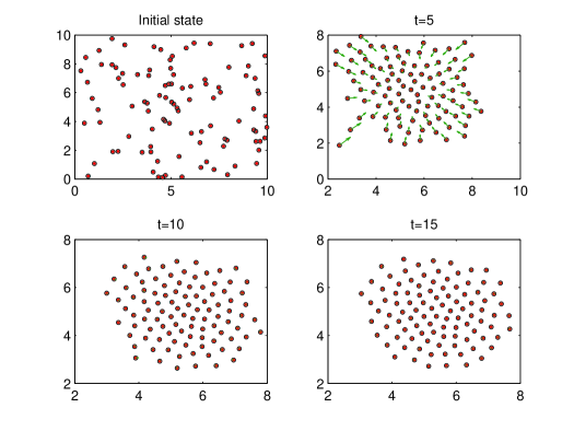
Figure 1: Schooling in $2$-dim. space

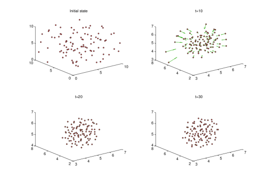
Figure 2: Schooling in $3$-dim. space

5.2 Collision

Let us next observe examples suggesting collision of two particles in the $d$-dimensional space, where $d=1,2$, with sufficiently small initial distance when $\sigma_{i}$ are not so small.

For the case $d=1$, we set $\alpha=5,\beta=1,r=0.5,p=3,q=4,\sigma_{i}=\sigma,$ and $F_{i}(t,x_{i},v_{i})=-v_{i}$. An initial value $\boldsymbol{x}(0)$ is generated randomly in $[0,1]^{2}$ and $\boldsymbol{v}(0)\equiv 0$. Figure 3 illustrates trajectories of two particles when $\sigma=0,0.15,5.$ If $\sigma$ is small (i.e., $\sigma=0,0.15$), collision does not take place. Meanwhile if $\sigma$ is large ($\sigma=5$), we observe that collision takes place.

For the case $d=2$, we set $\alpha=7,\beta=19,r=1,p=3,q=4,\sigma_{i}=9$, and $F_{i}(t,x_{i},v_{i})=-5v_{i}$. An initial value $\boldsymbol{x}(0)$ is generated randomly in $[0,5]^{4}$ and $\boldsymbol{v}(0)\equiv 0$. Figure 4 illustrates behavior of the distance of the two particles $x_{1}$ and $x_{2}$.

Figure 3: Collision in 1-dim. space

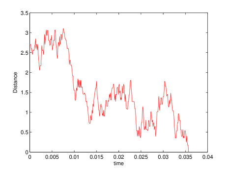
Figure 4: Collision in 2-dim. space

References

- [1] I. Aoki, A simulation study on the schooling mechanism in fish, Bull. Japanese Soc. Scientific Fisheries 48 (1982), 1081-1088.
- [2] L. Arnold, Stochastic Differential Equations: Theory and Applications, Wiley, New York, 1972.
- [3] S. Camazine, J. L. Deneubourg, N. R Franks, J. Sneyd, G. Theraulaz and E. Bonabeau, Self-Organization in Biological Systems, Princeton University Press, 2001.
- [4] M. R. D´Orsogna, Y. Chuang, A. Bertozzi, L. Chayes, Self-propelled particles with soft-core interactions: patterns, stability and collapse, Phys. Rev. Lett. 96 (2006), 104302.
- [5] A. Friedman, Stochastic Differential Equations and their Applications, Academic press, New York, 1976.
- [6] A. Huth and C. Wissel, The simulation of the movement of fish school, J. Theor. Biol. 156 (1992), 365-385.
- [7] T. Oboshi, S. Kato, A. Mutoh, H. Itoh, Collective or scattering: evolving schooling behaviors to escape from predator, Artificial Life, MIT Press, Cambridge, MA, VIII (2002), 386-389.
- [8] R. Olfati-saber, Flocking for multi-agent dynamic systems: Algorithms and theory, IEEE Trans. Automat. Control, 51 (2006), 401-420.
- [9] C. W. Reynolds, Flocks, herds, and schools: a distributed behavioral model, Computer Graphics 21 (1987), 25-34.
- [10] T. Vicsek, A. Czirók, E. Ben-Jacob, I. Cohen, and O. Shochet, Novel type of phase transition in a system of self-driven particles, Phys. Rev. Lett., 75 (1995), 1226-1229.
- [11] K. Warburton and J. Lazarus, Tendency-distance models of social cohesion in animal groups, J. Theor. Biol. 150 (1991), 473-488.