Skolem Functions for Factored Formulas

Abstract

Given a propositional formula $F(x,y)$, a Skolem function for $x$ is a function $\psi(y)$, such that substituting $\psi(y)$ for $x$ in $F$ gives a formula semantically equivalent to $\exists x~{}F$. Automatically generating Skolem functions is of significant interest in several applications including certified QBF solving, finding strategies of players in games, synthesising circuits and bit-vector programs from specifications, disjunctive decomposition of sequential circuits, etc. In many such applications, $F$ is given as a conjunction of factors, each of which depends on a small subset of variables. Existing algorithms for Skolem function generation ignore any such factored form and treat $F$ as a monolithic function. This presents scalability hurdles in medium to large problem instances. In this paper, we argue that exploiting the factored form of $F$ can give significant performance improvements in practice when computing Skolem functions. We present a new CEGAR style algorithm for generating Skolem functions from factored propositional formulas. In contrast to earlier work, our algorithm neither requires a proof of QBF satisfiability nor uses composition of monolithic conjunctions of factors. We show experimentally that our algorithm generates smaller Skolem functions and outperforms state-of-the-art approaches on several large benchmarks.

I Introduction

Skolem functions, introduced by Thoralf Skolem in the 1920s, occupy a central role in mathematical logic. Formally, let $F(x,y)$ be a first-order logic formula, and let $\operatorname{dom}(x)$ and $\operatorname{dom}(y)$ denote the domains of $x$ and $y$ respectively. A Skolem function for $x$ in $F$ is a function $\psi:\operatorname{dom}(y)\rightarrow\operatorname{dom}(x)$ such that substituting $\psi(y)$ for $x$ in $F$ yields a formula semantically equivalent to $\exists xF(x,y)$, i.e. $F(\psi(y),y)\equiv\exists xF(x,y)$. In this paper, we focus on the case where the formula $F$ is propositional and given as a conjunction of factors. Classically, Skolem functions have been used in proving theorems in logic. More recently, with the advent of fast SAT/SMT solvers, it has been shown that several practically relevant problems can be encoded as quantified formulas, and can be solved by constructing realizers of quantified variables. We identify these realizers as specific instances of Skolem functions, and focus on algorithms for constructing them in this paper.

We begin by listing some applications that illustrate the utility of constructing instances of Skolem functions in practice.

1. Quantifier elimination. Given a quantified formula $Qx~{}F(x,y)$, where $Q\in\{\exists,\forall\}$, the quantifier elimination problem requires us to find a quantifier-free formula that is semantically equivalent to $Qx~{}F(x,y)$. Quantifier elimination has important applications in diverse areas (see, e.g. [7, 14, 2] for a sampling). It follows from the definition of Skolem function that eliminating the quantifier from $\exists xF(x,y)$ can be achieved by substituting $x$ with a Skolem function for $x$. Since $\forall xF(x,y)$ can be written as $\neg\exists x\neg F(x,y)$, the same idea applies in this case too. In fact, the process can be repeated in principle to eliminate quantifiers from a formula with arbitrary quantifier prefix.

2. Controller Synthesis and Games. Control-program synthesis in the Ramadge-Wonham [12] framework reduces to games between two players—environment and the controller—such that the optimal strategy of the controller corresponds to an optimal control program. The optimal (or winning) strategy of the controller corresponds to choosing values of variables controlled by it such that regardless of the way the environment fixes its variables, the resulting play satisfies the controller’s objective. If the rules of the game are encoded as a propositional formula and if the strategy space for both players is finite, the optimal strategy of the controller corresponds to finding Skolem functions of variables controlled by it. In fact, for a number of two-player games—such as reachability games and safety games [2], tic-tac-toe [5] and chess-like games [3, 2]—the problem of deciding a winner can be reduced to checking satisfiability of a quantified Boolean formula (QBF), and the problem of finding winning or best-effort strategy reduces to Skolem function generation.

3. Graph Decomposition. Skolem functions can be used to compute disjunctive decompositions of implicitly specified state transition graphs of sequential circuits [16]. The disjunctive decomposition problem asks the following question: Given a sequential circuit, derive “component” sequential circuits, each of which has the same state space as the original circuit, but only a subset of transitions going out of every state. The components should be such that the complete set of state transitions of the original circuit is the union of the sets of state transitions of the components. Disjunctive decompositions have been shown to be useful in efficient reachability analysis [15].

There are several other practical applications where Skolem functions find use; see, e.g. [11], for a discussion. Hence, there is a growing need for practically efficient and scalable approaches for generating instances of Skolem functions. Large and complex representations of the formula $F$ in $\exists x~{}F$ often present scalability hurdles in generating Skolem functions in practice. Interestingly, for several problem instances, the specification of $F$ is available in a factored form, i.e., as a conjunction of simpler sub-formulas, each of which depends on a subset of variables appearing in $F$. Unfortunately, unlike in the case of disjunction, existential quantification does not distribute over conjunction of sub-formulas. Existing algorithms therefore ignore any factored form of $F$ and treat the conjunction of factors as a single monolithic function. We show in this paper that exploiting the factored form can help significantly when generating Skolem functions.

Our main technical contribution is a SAT-based Counter-Example Guided Abstraction-Refinement (CEGAR) algorithm for generating Skolem functions from factored formulas. Unlike competing approaches, our algorithm exploits the factored representation of a formula and leverages advances made in SAT-solving technology. The factored representation is used to arrive at an initial abstraction of Skolem functions, while a SAT-solver is used as an oracle to identify counter-examples that are used to refine the Skolem functions until no counter-examples exist. We present a detailed experimental evaluation of our algorithm vis-a-vis state-of-the-art algorithms [7, 11] over a large class of benchmarks. We show that on several large problem instances, we outperform competing algorithms.

Related Work. We are not aware of other techniques for Skolem function generation that exploit the factored form of a formula. Earlier work on Skolem function generation broadly fall in one of four categories. The first category includes techniques that extract Skolem functions from a proof of validity of $\exists X~{}F(X,Y)$ [11, 8, 4, 9]. In problem instances where $\exists X~{}F(X,Y)$ is valid (and this forms an important sub-class of problems), these techniques can usually find succinct Skolem functions if there exists a short proof of validity. However, in several other important classes of problems, the formula $\exists X~{}F(X,Y)$ does not evaluate to true for all values of $Y$, and techniques in the first category cannot be applied. The second category includes techniques that use templates for candidate Skolem functions [14]. These techniques are effective only when the set of candidate Skolem functions is known and small. While this is a reasonable assumption in some domains [14], it is not in most other domains. BDD-based techniques [13] are yet another way to compute Skolem functions. Unfortunately, these techniques are known not to scale well, unless custom-crafted variable orders are used. The last category includes techniques that use cofactors to obtain Skolem functions [7, 16]. These techniques do not exploit the factored representation of a formula and, as we show experimentally, do not scale well to large problem instances.

II Preliminaries

We use lower case letters (possibly with subscripts) to denote propositional variables, and upper case letters to denote sequences of such variables. We use $0$ and $1$ to denote the propositional constants false and true, respectively. Let $F(X,Y)$ be a propositional formula, where $X$ and $Y$ denote the sequences of variables $(x_{1},\ldots,x_{n})$ and $(y_{1},\ldots,y_{m})$, respectively. We are interested in problem instances where $F(X,Y)$ is given as a conjunction of factors $f^{1}(X_{1},Y_{1}),\ldots,f^{r}(X_{r},Y_{r})$, where each $X_{i}$ (resp., $Y_{i}$) is a possibly empty sub-sequence of $X$ (resp., $Y$). For notational convenience, we use $F$ and $\bigwedge_{j=1}^{r}f^{j}$ interchangeably throughout this paper. The set of variables in $F$ is called the support of $F$, and is denoted $\mathsf{Supp}(F)$. Given a propositional formula $F(X)$ and a propositional function $\Psi(X)$, we use $F[x_{i}/\Psi(X)]$, or simply $F[x_{i}/\Psi]$, to denote the formula obtained by substituting every occurrence of the variable $x_{i}$ in $F$ with $\Psi(X)$. Since the notions of formulas and functions coincide in propositional logic, the above is also conventionally called function composition. If $X$ is a sequence of variables and $x_{i}$ is a variable, we use $X\setminus x_{i}$ to denote the sub-sequence of $X$ obtained by removing $x_{i}$ (if present) from $X$. Abusing notation, we use $X$ to also denote the set of elements in $X$, when there is no confusion. A valuation or assignment $\pi$ of $X$ is a mapping $\pi:X\rightarrow\{0,1\}$.

Definition 1.

Given a propositional formula $F(X,Y)$ and a variable $x_{i}\in X$, a Skolem function for $x_{i}$ in $F(X,Y)$ is a function $\psi(X\setminus x_{i},Y)$ such that $\exists x_{i}~{}F\equiv F[x_{i}/\psi]$.

A Skolem function for $x_{i}$ in $F$ need not be unique. The following proposition, which effectively follows from [7, 16], characterizes the space of all Skolem functions for $x_{i}$ in $F$.

Proposition 1.

A function $\psi(X\setminus x_{i},Y)$ is a Skolem function for $x_{i}$ in $F(X,Y)$ iff $F[x_{i}/1]\wedge\neg F[x_{i}/0]\Rightarrow\psi$ and $\psi\Rightarrow F[x_{i}/1]\vee\neg F[x_{i}/0]$.

The function $F[x_{i}/0]$ (resp., $F[x_{i}/1]$) is called the positive (resp., negative) cofactor of $F$ with respect to $x_{i}$, and plays a central role in the study of Skolem functions for propositional formulas. In particular, it follows from Proposition 1 that $F[x_{i}/1]$ is a Skolem function for $x_{i}$ in $F$. The above definition for a single variable can be naturally extended to a vector of variables. Given $F(X,Y)$, a Skolem function vector for $X=(x_{1},\ldots,x_{n})$ in $F$ is a vector of functions $\mathbf{\Psi}=(\psi_{1},\ldots,\psi_{n})$ such that $\exists x_{1}\ldots x_{n}~{}F\equiv$ $(\cdots(F[x_{1}/\psi_{1}])\cdots[x_{n}/\psi_{n}])$. A straightforward way to obtain a Skolem function vector $\mathbf{\Psi}$ is to first obtain a Skolem function $\psi_{1}$ for $x_{1}$ in $F$, then compute $F^{\prime}\equiv\exists x_{1}\,F$ and obtain a Skolem function $\psi_{2}$ for $x_{2}$ in $F^{\prime}$, and so on until $\psi_{n}$ has been obtained. More formally, $\psi_{i}$ can be computed as a Skolem function for $x_{i}$ in $\exists x_{1}\ldots x_{i-1}\,F$, starting from $\psi_{1}$ and proceeding to $\psi_{n}$. Note that $\exists x_{1}\ldots x_{i-1}\,F$ can itself be computed as $\left(\cdots\left(F[x_{1}/\psi_{1}]\right)\cdots[x_{i-1}/\psi_{i-1}]\right)$.

Definition 2.

The “$\mathbf{C}$an’t-$\mathbf{b}$e-$\mathbf{1}$” function for $x_{i}$ in $F$, denoted ${\mathtt{Cb{1}}[{x_{i}}]}(F)$, is defined to be $\left(\neg\exists x_{1}\ldots x_{i-1}\,F\right)[x_{i}/1]$. Similarly, the “$\mathbf{C}$an’t-$\mathbf{b}$e-$\mathbf{0}$” function for $x_{i}$ in $F$, denoted ${\mathtt{Cb{0}}[{x_{i}}]}(F)$, is defined to be $\left(\neg\exists x_{1}\ldots x_{i-1}\,F\right)[x_{i}/0]$. When $X$ and $F$ are clear from the context, we use ${\mathtt{Cb{1}}[{i}]}$ and ${\mathtt{Cb{0}}[{i}]}$ for ${\mathtt{Cb{1}}[{x_{i}}]}(F)$ and ${\mathtt{Cb{0}}[{x_{i}}]}(F)$, respectively.

Intuitively, in order to make $F$ evaluate to $1$, we cannot set $x_{i}$ to $1$ (resp. $0$) whenever the valuation of $\left\{x_{i+1},\ldots,x_{n}\right\}\cup Y$ satisfies ${\mathtt{Cb{1}}[{i}]}$ (resp., ${\mathtt{Cb{0}}[{i}]}$). The following proposition follows from Definition 2 and from our observation about computing a Skolem function vector one component at a time.

Proposition 2.

$\mathbf{\Psi}{=}(\neg{\mathtt{Cb{1}}[{1}]},\ldots,\neg{\mathtt{Cb{1}}[{n}]})$ is a Skolem function vector for $X$ in $F$.

Note that the support of $\psi_{i}$ in $\mathbf{\Psi}$, as given by Proposition 2, is $\left\{x_{i+1},\ldots,x_{n}\right\}\cup Y$. If we want a Skolem function vector $\mathbf{\Psi}$ such that every component function has only $Y$ (or a subset thereof) as support, this can be obtained by repeatedly substituting the Skolem function for every variable $x_{i}$ in all other Skolem functions where $x_{i}$ appears. We denote such a Skolem function vector as $\mathbf{\Psi}(Y)$.

III A monolithic composition based algorithm

Our algorithm is motivated in part by cofactor-based techniques for computing Skolem functions, as proposed by Jiang et al [7] and Trivedi [16]. Given $F(X,Y)=\bigwedge_{j=1}^{r}f^{j}(X_{j},Y_{j})$, the techniques of [7, 16] essentially compute a Skolem function vector $\mathbf{\Psi}(Y)$ for $X$ in $F$ as shown in algorithm MonoSkolem (see Algorithm 1). In this algorithm, the variables in $X$ are assumed to be ordered by their indices. While variable ordering is known to affect the difficulty of computing Skolem functions [7], we assume w.l.o.g. that the variables are indexed to represent a desirable order. We describe the variable order used in our study later in Section V.

MonoSkolem works in two phases. In the first phase, it implements a straightforward strategy for obtaining a Skolem function vector, as suggested by Proposition 2. Specifically, steps $3$ and $4$ of MonoSkolem build a monolithic conjunction $F_{i}$ of all factors that have $x_{i}$ in their support, before computing $\psi_{i}$. This restricts the scope of the quantifier for $x_{i}$ to the conjunction of these factors. In Step $6$, we use $\neg{\mathtt{Cb{1}}[{i}]}$ as a specific choice for the Skolem function $\psi_{i}$. After computing $\psi_{i}$ from $F_{i}$, step $7$ discards the factors with $x_{i}$ in their support, and introduces a single factor representing $\exists x_{i}\,F_{i}$ (computed as $F_{i}[x_{i}/\psi_{i}]$) in their place. Note that each $\psi_{i}$ obtained in this manner has $\left\{x_{i+1},\ldots,x_{n}\right\}\cup Y$ (or a subset thereof) as support. Since we want each Skolem function to have support $Y$, a second phase of “reverse” substitutions is needed. In this phase (see Algorithm 2), the Skolem function $\psi_{n}(Y)$ obtained above is substituted for $x_{n}$ in $\psi_{1},\ldots,\psi_{n-1}$. This effectively renders all Skolem functions independent of $x_{n}$. The process is then repeated with $\psi_{n-1}$ substituted for $x_{n-1}$ in $\psi_{1},\ldots,\psi_{n-2}$ and so on, until all Skolem functions have been made independent of $x_{1},\ldots,x_{n}$, and have only $Y$ (or subsets thereof) as support.

MonoSkolem can be further refined by combining steps 5 and 6, and directly defining $\psi_{i}$ in terms of $F_{i}$. However, we introduce the intermediate step using ${\mathtt{Cb{0}}[{i}]}$ and ${\mathtt{Cb{1}}[{i}]}$ to motivate their central role in our approach. Note that instead of $\neg{\mathtt{Cb{1}}[{i}]}$, we could combine ${\mathtt{Cb{1}}[{i}]}$ and ${\mathtt{Cb{0}}[{i}]}$ in other ways (denoted by Combine(${\mathtt{Cb{0}}[{i}]},{\mathtt{Cb{1}}[{i}]}$) within comments in Algorithm 1) to get $\psi_{i}$ in Step $6$. In fact, Jiang et al [7] compute a Skolem function for $x_{i}$ in $F$ as an interpolant of $\neg{\mathtt{Cb{1}}[{i}]}\wedge{\mathtt{Cb{0}}[{i}]}$ and ${\mathtt{Cb{1}}[{i}]}\wedge\neg{\mathtt{Cb{0}}[{i}]}$, while Trivedi [16] observes that the function $(\neg{\mathtt{Cb{1}}[{i}]}\wedge({\mathtt{Cb{0}}[{i}]}\vee g))\;\vee\;({\mathtt{Cb{1}}[{i}]}\wedge{\mathtt{Cb{0}}[{i}]}\wedge h)$ serves as a Skolem function for $x_{i}$ in $F$ where $h$ and $g$ are arbitrary propositional functions with support in $X\setminus\left\{x_{i}\right\}\cup Y$. Since computing interpolants using a SAT solver is often time-intensive and does not always lead to succinct Skolem functions [7], we simply use $\neg{\mathtt{Cb{1}}[{i}]}$ as a Skolem function in Step $6$. Proposition 2 guarantees the correctness of this choice.

Input: Prop. formula $F(X,Y)=\bigwedge_{j=1}^{r}f^{j}(X_{j},Y_{j})$, where $X=(x_{1},\ldots,x_{n})$

Output: Skolem function vector $\mathbf{\Psi}(Y)$

// Phase 1 of algorithm

1 $\mathsf{Factors}:=\left\{f^{j}\>:\>1\leq j\leq r\right\}$;

2 for $i$ in $1$ to $n$ do

3       $\mathsf{FactorsWithXi}:=\left\{f\>:\>f\in\mathsf{Factors},x_{i}\in\mathsf{Supp}(f)\right\}$;

4       $F_{i}:=\bigwedge_{f\in\mathsf{FactorsWithXi}}f$;

5       ${\mathtt{Cb{0}}[{i}]}:=\neg F_{i}[x_{i}/0]$; ${\mathtt{Cb{1}}[{i}]}:=\neg F_{i}[x_{i}/1]$;

6       $\psi_{i}:=$ $\neg{\mathtt{Cb{1}}[{i}]}$;

       // Generally, $\psi_{i}$:=Combine(${\mathtt{Cb{0}}[{i}]},{\mathtt{Cb{1}}[{i}]}$);

7       $\mathsf{Factors}:=$ $\left(\mathsf{Factors}\setminus\mathsf{FactorsWithXi}\right)\cup\left\{F_{i}[x_{i}/\psi_{i}]\right\}$;

8      

// Phase 2 of algorithm

9 return ReverseSubstitute($\psi_{1},\ldots,\psi_{n}$);

Algorithm 1 MonoSkolem

Input: Functions $\psi_{1}(x_{2},\ldots,x_{n},Y),\psi_{2}(x_{3},\ldots,x_{n},Y),\ldots,\psi_{n}(Y)$

Output: Function vector $\mathbf{\Psi}(Y)$

1 for $i=n$ downto $2$ do

2       for $k=i-1$ downto $1$ do $\psi_{k}$ = $\psi_{k}[x_{i}/\psi_{i}]$;

3      

4return $\mathbf{\Psi}(Y)=(\psi_{1}(Y),\ldots,\psi_{n}(Y))$;

Algorithm 2 ReverseSubstitute

Observe that MonoSkolem works with a monolithic conjunction ($F_{i}$) of factors that have $x_{i}$ in their support. Specifically, it composes each such monolithic conjunction $F_{i}$ with a cofactor of $F_{i}$ in Step $7$ to eliminate quantifiers sequentially. This can lead to large memory footprints and more time-outs when used with medium to large benchmarks, as confirmed by our experiments. This motivates us to ask if we can develop a cofactor-based algorithm that does not suffer from the above drawbacks of MonoSkolem.

IV CEGAR for generating Skolem functions

We now present a new CEGAR [6] algorithm for generating Skolem function vectors, that exploits the factored form of $F(X,Y)$. Like MonoSkolem, our new algorithm, named CegarSkolem, works in two phases, and assumes that the variables in $X$ are ordered by their indices. The first phase of the algorithm consists of the core abstraction-refinement part, and computes a Skolem function vector $(\psi_{1},\ldots,\psi_{n})$, where $\psi_{i}$ has $\left\{x_{i+1},\ldots,x_{n}\right\}\cup Y$, or a subset thereof, as support. Unlike in MonoSkolem, this phase avoids composing monolithic conjunctions of factors, yielding simpler Skolem functions. The second phase of the algorithm performs reverse substitutions, similar to that in MonoSkolem.

Before describing the details of CegarSkolem, we introduce some additional notation and terminology. Given propositional functions (or formulas) $f$ and $g$, we say that $f$ refines $g$ and $g$ abstracts $f$ iff $f$ logically implies $g$. Given $F(X,Y)$ and a vector of functions ${\mathbf{\Psi^{A}}}=({\psi_{{1}}^{A}},\ldots,{\psi_{{n}}^{A}})$, we say that ${\mathbf{\Psi^{A}}}$ is an abstract Skolem function vector for $X$ in $F$ iff there exists a Skolem function vector $\mathbf{\Psi}=(\psi_{1},\ldots,\psi_{n})$ for $X$ in $F$ such that $~{}{\psi_{{i}}^{A}}$ abstracts $\psi_{i}$, for every $i\in\left\{1,\ldots,n\right\}$. Instead of using ${\mathtt{Cb{0}}[{i}]}$ and ${\mathtt{Cb{1}}[{i}]}$ to compute Skolem functions, as was done in MonoSkolem, we now use their refinements, denoted ${\mathtt{r{0}}}[{i}]$ and ${\mathtt{r{1}}}[{i}]$ respectively, to compute abstract Skolem functions. For convenience, we represent ${\mathtt{r{0}}}[{i}]$ and ${\mathtt{r{1}}}[{i}]$ as sets of implicitly disjoined functions. Thus, if ${\mathtt{r{1}}}[{i}]$, viewed as a set, is $\left\{g_{1},g_{2}\right\}$, then it is $g_{1}\vee g_{2}$ when viewed as a function. We abuse notation and use ${\mathtt{r{1}}}[{i}]$ (resp., ${\mathtt{r{0}}}[{i}]$) to denote a set of functions or their disjunction, as needed.

IV-A Overview of our CEGAR algorithm

Algorithm CegarSkolem has two phases. The first phase consists of a CEGAR loop, while the second does reverse substitutions. The CEGAR loop has the following steps.

• Initial abstraction and refinement. This step involves constructing refinements of ${\mathtt{Cb{0}}[{i}]}$ and ${\mathtt{Cb{1}}[{i}]}$ for every $x_{i}$ in $X$. Using Proposition 2, we can then construct an initial abstract Skolem function vector ${\mathbf{\Psi^{A}}}$. This step is implemented in Algorithm 3 (InitAbsRef), which processes individual factors of $F(X,Y)=\bigwedge_{j=1}^{r}f^{j}(X_{j},Y_{j})$ separately, without considering their conjunction. As a result, this step is time and memory efficient if the individual factors are simple with small representations.

• Termination Condition. Once InitAbsRef has computed ${\mathbf{\Psi^{A}}}$, we check whether ${\mathbf{\Psi^{A}}}$ is already a Skolem function vector. This is achieved by constructing an appropriate propositional formula $\varepsilon$, called the “error formula” for ${\mathbf{\Psi^{A}}}$ (details in Subsection IV-C), and checking for its satisfiability. An unsatisfiable formula implies that ${\mathbf{\Psi^{A}}}$ is a Skolem function vector. Otherwise, a satisfying assignment $\pi$ of $\varepsilon$ is used to improve the current refinements of ${\mathtt{Cb{1}}[{i}]}$ and ${\mathtt{Cb{0}}[{i}]}$ for suitable variables $x_{i}$.

• Counterexample guided abstraction and refinement. This step is implemented in Algorithm 4: UpdateAbsRef, and computes an improved (i.e., more abstract) refinement of ${\mathtt{Cb{0}}[{i}]}$ and ${\mathtt{Cb{1}}[{i}]}$ for some $x_{i}\in X$. This, in turn, leads to a refinement of the abstract Skolem function vector ${\mathbf{\Psi^{A}}}$.

The overall CEGAR loop starts with the first step and repeats the second and third steps until a Skolem function vector is obtained. We now discuss the three steps in detail.

IV-B Initial Abstraction and Refinement

Input: Prop. formula $F(X,Y)=\bigwedge_{j=1}^{r}f^{j}(X_{j},Y_{j})$, where $X=(x_{1},\ldots,x_{n})$

Output: Abstract Skolem function vector ${\mathbf{\Psi^{A}}}=({\psi_{{1}}^{A}},\ldots,{\psi_{{n}}^{A}})$, and refinements ${\mathtt{r{0}}}[{i}]$ and ${\mathtt{r{1}}}[{i}]$ for each $x_{i}$ in $X$

1 for $i$ in $1$ to $n$ do

      ${\mathtt{r{0}}}[{i}]$ := $\emptyset$; ${\mathtt{r{1}}}[{i}]$ := $\emptyset$; // Initializing

2      

3for $j$ in $1$ to $r$ do

       $f:=f^{j}$; // for each factor

4       for $i$ in $1$ to $n$ do

5             if $x_{i}\in\mathsf{Supp}(f)$ then

6                   ${\mathtt{r{0}}}[{i}]:={\mathtt{r{0}}}[{i}]\cup\left\{\neg f[x_{i}/0]\right\}$;

7                   ${\mathtt{r{1}}}[{i}]:={\mathtt{r{1}}}[{i}]\cup\left\{\neg f[x_{i}/1]\right\}$;

                   // Skolem function for $x_{i}$ in $f$

8                   $\psi_{i,f}:=f[x_{i}/1]$;

                   $f:=f[x_{i}/\psi_{i,f}]$; // $\because f[x_{i}/\psi_{i,f}]\equiv\exists x_{i}\,f$

9                  

10            

11      

12

13for $i$ in $1$ to $n$ do

14       ${\psi_{{i}}^{A}}:=\neg{\mathtt{r{1}}}[{i}]$;

       // Interpreting ${\mathtt{r{1}}}[{i}]$ as a function

15      

return ${\mathbf{\Psi^{A}}}{=}({\psi_{{1}}^{A}},\ldots,{\psi_{{n}}^{A}})$ and ${\mathtt{r{0}}}[{i}],{\mathtt{r{1}}}[{i}]$ $\forall x_{i}{\in}X$

Algorithm 3 InitAbsRef

Algorithm InitAbsRef (see Algorithm 3) starts by initializing each ${\mathtt{r{1}}}[{i}]$ and ${\mathtt{r{0}}}[{i}]$, viewed as sets, to the empty set. Subsequently, it considers each factor $f$ in $\bigwedge_{j=1}^{r}f^{j}(X_{j},Y_{j})$, and determines the contribution of $f$ to ${\mathtt{Cb{0}}[{i}]}$ and ${\mathtt{Cb{1}}[{i}]}$, for every $x_{i}$ in the support of $f$. Specifically, if $x_{i}\in\mathsf{Supp}(f)$, the contribution of $f$ to ${\mathtt{Cb{0}}[{i}]}$ is $\left(\neg\exists x_{1}\ldots x_{i-1}\,f\right)[x_{i}/0]$, and its contribution to ${\mathtt{Cb{1}}[{i}]}$ is $\left(\neg\exists x_{1}\ldots x_{i-1}\,f\right)[x_{i}/1]$. These contributions are accumulated in the sets ${\mathtt{r{0}}}[{i}]$ and ${\mathtt{r{1}}}[{i}]$, respectively, and $x_{i}$ is existentially quantified from $f$. The process is then repeated with the next variable in the support of $f$. Once the contributions from all factors are accumulated in ${\mathtt{r{0}}}[{i}]$ and ${\mathtt{r{1}}}[{i}]$ for each $x_{i}$ in $X$, InitAbsRef computes an abstract Skolem function ${\psi_{{i}}^{A}}$ for each $x_{i}$ in $F$ by complementing ${\mathtt{r{1}}}[{i}]$, interpreted as a disjunction of functions. Note that executing steps $4$ through $10$ of InitAbsRef for a specific factor $f$ is operationally similar to executing steps $1$ through $7$ of MonoSkolem with a singleton set of factors, i.e., $\mathsf{Factors}=\left\{f\right\}$. This highlights the key difference between InitAbsRef and MonoSkolem: while MonoSkolem works with monolithic conjunctions of factors and their compositions, InitAbsRef works with individual factors, without ever considering their conjunctions. Lemma 1 asserts the correctness of InitAbsRef.

Lemma 1.

The vector ${\mathbf{\Psi^{A}}}$ computed by InitAbsRef is an abstract Skolem function vector for $X$ in $F(X,Y)$. In addition, ${\mathtt{r{0}}}[{i}]$ and ${\mathtt{r{1}}}[{i}]$ computed by InitAbsRef are refinements of ${\mathtt{Cb{0}}[{i}]}(F)$ and ${\mathtt{Cb{1}}[{i}]}(F)$ for every $x_{i}$ in $X$.

Proof.

Consider the ordered pair $(j,i)$ of loop indices corresponding to the nested loops in steps $3-10$ and $5-10$ of algorithm InitAbsRef. Every update of ${\mathtt{r{0}}}[{i}]$ and ${\mathtt{r{1}}}[{i}]$ in steps $7$ and $8$ of InitAbsRef can be associated with a unique ordered pair of loop indices. Define a linear ordering $\preceq$ on the loop index pairs as: $(j,i)\preceq(j^{\prime},i^{\prime})$ iff $j<j^{\prime}$, or $j=j^{\prime}$ and $i\leq i^{\prime}$. Note that this represents the ordering of loop index pairs in successive iterations of the loop in steps $5-10$ of InitAbsRef. We use induction on $(j,i)$, ordered by $\preceq$, to show that ${\mathtt{r{0}}}[{i}]$ and ${\mathtt{r{1}}}[{i}]$, as computed by InitAbsRef, are refinements of ${\mathtt{Cb{0}}[{i}]}$ and ${\mathtt{Cb{1}}[{i}]}$. The base case follows from the initialization in steps $1$ and $2$ of InitAbsRef. To prove the inductive step, consider an update of ${\mathtt{r{0}}}[{i}]$ and ${\mathtt{r{1}}}[{i}]$ in steps $7$ and $8$, respectively, of InitAbsRef. The function $f$ used in steps $7$ and $8$ is easily seen to be $\exists x_{i}\ldots x_{i-1}\,f^{j}$. Since $f^{j}$ is a factor of $F$, we also have $F\Rightarrow f^{j}$. It follows that $\exists x_{i}\ldots x_{i-1}\,F\;\Rightarrow\;\exists x_{i}\ldots x_{i-1}\,f^{j}\;\equiv\;f$. Taking the contrapositive gives $\neg f\;\Rightarrow\;\neg\exists x_{i}\ldots x_{i-1}\,F$. Therefore, $\neg f[x_{i}/a]\Rightarrow(\neg\exists x_{1}\ldots x_{i-1}\,F)[x_{i}/a]$ for every propositional constant $a$. Recalling the definitions of ${\mathtt{Cb{0}}[{i}]}$ and ${\mathtt{Cb{1}}[{i}]}$, we get $\neg f[x_{i}/0]\Rightarrow{\mathtt{Cb{0}}[{i}]}$ and $\neg f[x_{i}/1]\Rightarrow{\mathtt{Cb{1}}[{1}]}$. By the inductive hypothesis, ${\mathtt{r{0}}}[{i}]$ and ${\mathtt{r{1}}}[{i}]$ are refinements of ${\mathtt{Cb{0}}[{i}]}$ and ${\mathtt{Cb{1}}[{i}]}$ prior to executing step $7$ of InitAbsRef. Therefore, the updated values of ${\mathtt{r{0}}}[{i}]$ and ${\mathtt{r{1}}}[{i}]$, as computed in steps $7$ and $8$ of InitAbsRef, are also refinements of ${\mathtt{Cb{0}}[{i}]}$ and ${\mathtt{Cb{1}}[{i}]}$. This completes the induction.

Since ${\mathtt{r{1}}}[{i}]\Rightarrow{\mathtt{Cb{1}}[{i}]}$ for every $x_{i}$ in $X$ when we reach step $11$ of InitAbsRef, it follows from Proposition 2 that ${\psi_{{i}}^{A}}=\neg{\mathtt{r{1}}}[{i}]$ abstracts a Skolem function for $x_{i}$ in $F$. Hence, ${\mathbf{\Psi^{A}}}$, as computed by InitAbsRef, is an abstract Skolem function vector for $X$ in $F$. ∎

IV-C Termination condition

Given $F(X,Y)$ and an abstract Skolem function vector ${\mathbf{\Psi^{A}}}$, it may happen that ${\mathbf{\Psi^{A}}}$ is already a Skolem function vector for $X$ in $F$. We therefore check if ${\mathbf{\Psi^{A}}}$ is a Skolem function vector before refinement. Towards this end, we define the error formula for ${\mathbf{\Psi^{A}}}$ as $F(X^{\prime},Y)\wedge\bigwedge_{i=1}^{n}(x_{i}\Leftrightarrow{\psi_{{i}}^{A}})\wedge\neg F(X,Y)$, where $X^{\prime}{=}(x_{1}^{\prime},\ldots,x_{n}^{\prime})$ is a sequence of fresh variables with no variable in common with $X$. The first term in the error formula checks if there exists some valuation of $X$ that renders $\exists YF(X,Y)$ true. The second term assigns variables in $X$ to the values given by the abstract Skolem functions, and the third term checks if this assignment falsifies the formula $F$.

Lemma 2.

The error formula for ${\mathbf{\Psi^{A}}}$ is unsatisfiable iff ${\mathbf{\Psi^{A}}}$ is a Skolem function vector of $X$ in $F$.

Proof.

Let $\varepsilon$ be the error formula for ${\mathbf{\Psi^{A}}}$. Suppose $\varepsilon$ is unsatisfiable. By definition of $\varepsilon$, we have

$$\forall Y\forall X^{\prime}\forall X\,\left(F(X^{\prime},Y)\Rightarrow\left(\bigwedge_{i=1}^{n}(x_{i}\Leftrightarrow{\psi_{{i}}^{A}})\;\;\Rightarrow\;\;F(X,Y)\right)\right).$$

By standard logic transformations, this implies $\forall Y\left(\exists X^{\prime}F(X^{\prime},Y)\,\Rightarrow\,F^{\prime}(Y)\right)$, where $F^{\prime}(Y)$ denotes $\left(\cdots\left(F[x_{1}/{\psi_{{1}}^{A}}]\right)\cdots[x_{n}/{\psi_{{n}}^{A}}]\right)$. Therefore, ${\mathbf{\Psi^{A}}}$ is a Skolem function vector for $X$ in $F$.

Suppose $\pi$ is a satisfying assignment of $\varepsilon$. By definition of $\varepsilon$, $\pi$ is a satisfying assignment of $F(X^{\prime},Y)$ and of $\bigwedge_{i=1}^{n}\left(x_{i}\Leftrightarrow{\psi_{{i}}^{A}}\right)\wedge\neg F(X,Y)$, considered separately. Thus, the values of $x_{1},\ldots,x_{n}$ given by ${\psi_{{1}}^{A}},\ldots,{\psi_{{n}}^{A}}$ respectively, cause $F$ to evaluate to $0$ for the valuation of $Y$ in $\pi$. However, there exists a valuation of $X$ (viz. same as that of $X^{\prime}$ in $\pi$) that causes $F$ to evaluate to $1$ for the same valuation of $Y$ in $\pi$. Hence, ${\mathbf{\Psi^{A}}}$ is not a Skolem function vector for $X$ in $F$, as witnessed by the valuation of $Y$ in $\pi$. ∎

The following example illustrates the role of the error formula.

Example 1.

Let $X=\{x_{1},x_{2}\}$, $Y=\{y_{1},y_{2},y_{3}\}$ in $\exists x_{1}x_{2}F(X,Y)$ where $F\equiv(f_{1}\wedge f_{2}\wedge f_{3})$, with $f_{1}=(\neg x_{1}\vee\neg x_{2}\vee\neg y_{1})$, $f_{2}=(x_{2}\vee\neg y_{3}\vee\neg y_{2})$, $f_{3}=(x_{1}\vee\neg x_{2}\vee y_{3})$.

Algorithm InitAbsRef gives ${\mathtt{r{1}}}[{1}]=(x_{2}\wedge y_{1})$, ${\mathtt{r{0}}}[{1}]=(x_{2}\wedge\neg y_{3})$, ${\mathtt{r{1}}}[{2}]=\textsf{false}$, ${\mathtt{r{0}}}[{2}]=y_{3}\wedge y_{2}$. This yields ${\psi_{{1}}^{A}}=(\neg x_{2}\vee\neg y_{1})$, ${\psi_{{2}}^{A}}=\textsf{true}$. Now, while ${\psi_{{1}}^{A}}$ is a correct Skolem function for $x_{1}$ in $F$, ${\psi_{{2}}^{A}}$ is not for $x_{2}$. This is detected by the satisfiability of the error formula $\varepsilon=F(x^{\prime}_{1},x^{\prime}_{2},Y)\wedge(x_{1}=\neg x_{2}\vee\neg y_{1})\wedge(x_{2}=1)\wedge\neg F(x_{1},x_{2},Y)$. Note that $\neg F(\neg x_{2}\vee\neg y_{1},1,Y)$ simplifies to $(y_{1}\wedge\neg y_{3})$, and $y_{1}=1,y_{2}=1,y_{3}=0,x_{1}=0,x_{2}=1,x_{1}^{\prime}=0,x_{2}^{\prime}=0$ is a satisfying assignment for $\varepsilon$.

IV-D Counterexample-guided abstraction and refinement

Let $\varepsilon$ be the error formula for ${\mathbf{\Psi^{A}}}$, and let $\pi$ be a satisfying assignment of $\varepsilon$. We call $\pi$ a counterexample of the claim that ${\mathbf{\Psi^{A}}}$ is a Skolem function vector. For every variable $v\in X^{\prime}\cup X\cup Y$, we use $\pi(v)$ to denote the value of $v$ in $\pi$. Satisfiability of $\varepsilon$ implies that we need to refine at least one abstract Skolem function ${\psi_{{i}}^{A}}$ in ${\mathbf{\Psi^{A}}}$ to make it a Skolem function vector. Since ${\psi_{{i}}^{A}}$ is $\neg{\mathtt{r{1}}}[{i}]$ in our approach, refining ${\psi_{{i}}^{A}}$ can be achieved by computing an improved (i.e., more abstract) version of ${\mathtt{r{1}}}[{i}]$. Algorithm UpdateAbsRef implements this idea by using $\pi$ to determine which ${\mathtt{r{1}}}[{i}]$ should be rendered abstract by adding appropriate functions to ${\mathtt{r{1}}}[{i}]$, viewed as a set.

Before delving into the details of UpdateAbsRef, we state some key results. In the following, we use $\pi\models f$ to denote that the formula $f$ evaluates to $1$ when the variables in $\mathsf{Supp}(f)$ are set to values given by $\pi$. If $\pi\models f$, we also say $f$ evaluates to $1$ under $\pi$. We use ${\mathtt{r{0}}}[{i}]_{init}$ and ${\mathtt{r{1}}}[{i}]_{init}$ to refer to ${\mathtt{r{0}}}[{i}]$ and ${\mathtt{r{1}}}[{i}]$, as computed by algorithm InitAbsRef. Since UpdateAbsRef only adds to ${\mathtt{r{1}}}[{i}]$ and ${\mathtt{r{0}}}[{i}]$ viewed as sets, it is easy to see that ${\mathtt{r{0}}}[{i}]_{init}\Rightarrow{\mathtt{r{0}}}[{i}]$ and ${\mathtt{r{1}}}[{i}]_{init}\Rightarrow{\mathtt{r{1}}}[{i}]$ viewed as functions (recall these functions are simply disjunctions of elements in the corresponding sets).

Lemma 3.

Let $\pi$ be a satisfying assignment of the error formula $\varepsilon$ for ${\mathbf{\Psi^{A}}}$. Then the following hold.

1. $\pi\models\neg{\mathtt{Cb{0}}[{n}]}\vee\neg{\mathtt{Cb{1}}[{n}]}$.

2. There exists $k\in\{1,\ldots,n-1\}$ s.t., $\pi\models{\mathtt{r{1}}}[{k}]\wedge{\mathtt{r{0}}}[{k}]$.

3. There exists no Skolem function vector $\mathbf{\Psi}=(\psi_{1},\ldots,\psi_{n})$ such that $\psi_{j}\Leftrightarrow{\psi_{{j}}^{A}}$ for all $j$ in $\left\{k+1,\ldots,n\right\}$.

4. There exists $l\in\{k+1,\ldots,n\}$ such that $x_{l}=1$ in $\pi$, and $\pi\models{\mathtt{Cb{1}}[{l}]}\wedge\neg{\mathtt{r{0}}}[{l}]$.

Proof.

Part (a): Consider an assignment $\pi^{\prime}$ of variables in $X\cup Y$, such that $\pi^{\prime}(x_{i})=\pi(x_{i}^{\prime})$ for all $x_{i}\in X$, and $\pi^{\prime}(y_{j})=\pi(y_{j})$ for all $y_{j}\in Y$. Since $\pi\models\varepsilon$, by definition of $\varepsilon$, we have $\pi\models F(X^{\prime},Y)$. This implies that $\pi^{\prime}\models F(X,Y)$ and hence, $\pi^{\prime}\models\exists x_{1}\ldots x_{n-1}\,F$. If $x_{n}=1$ in $\pi^{\prime}$, we get $\pi^{\prime}\models\left(\exists x_{1}\ldots x_{n-1}\,F\right)[x_{n}/1]$, or equivalently, $\pi^{\prime}\models\neg{\mathtt{Cb{1}}[{n}]}$. If $x_{n}=0$ in $\pi^{\prime}$, by a similar argument, $\pi^{\prime}\models\neg{\mathtt{Cb{0}}[{n}]}$. Therefore, $\pi^{\prime}\models\neg{\mathtt{Cb{1}}[{n}]}\vee\neg{\mathtt{Cb{0}}[{n}]}$. Since $x_{n}$ is the variable with the highest index in $X$, both ${\mathtt{Cb{1}}[{n}]}$ and ${\mathtt{Cb{0}}[{n}]}$ have only $Y$ as their support. Since $\pi^{\prime}(y_{j})=\pi(y_{j})$ for all $y_{j}\in Y$, it follows that $\pi\models\neg{\mathtt{Cb{1}}[{n}]}\vee\neg{\mathtt{Cb{0}}[{n}]}$ as well.

Part (b): Since $\pi\models\varepsilon$, by definition of $\varepsilon$, we have $\pi\models\neg F(X,Y)$. Since $F=\bigwedge_{q=1}^{r}f^{q}$, there exists $j\in\{1,\ldots,r\}$ such that $\pi\models\neg f^{j}$. Without loss of generality, assume that $\mathsf{Supp}(f^{j})\neq\emptyset$ (otherwise, $f^{j}$ can be removed from $\bigwedge_{q=1}^{r}f^{q}$). Let $x_{k}$ be the variable with the smallest index in $\mathsf{Supp}(f^{j})$. We claim that $x_{k}=0$ in $\pi$, and prove this by contradiction.

If possible, let $x_{k}=1$ in $\pi$. Then, $\pi\models(\neg f^{j})[x_{k}/1]$. Since $x_{k}$ is the lowest indexed variable in $\mathsf{Supp}(f^{j})$, it follows from algorithm InitAbsRef that $(\neg f^{j})[x_{k}/1]\in{\mathtt{r{1}}}[{k}]_{init}$, when ${\mathtt{r{1}}}[{k}]_{init}$ is viewed as a set. This implies that $(\neg f^{j})[x_{k}/1]\Rightarrow{\mathtt{r{1}}}[{k}]_{init}$, when ${\mathtt{r{1}}}[{k}]_{init}$ is viewed as a function. Hence, $\pi\models{\mathtt{r{1}}}[{k}]_{init}$, and since ${\mathtt{r{1}}}[{k}]_{init}\Rightarrow{\mathtt{r{1}}}[{k}]$, we have $\pi\models{\mathtt{r{1}}}[{k}]$. By definition of $\varepsilon$, we also have $\pi\models(x_{k}\Leftrightarrow{\psi_{{k}}^{A}})$, where ${\psi_{{k}}^{A}}=\neg{\mathtt{r{1}}}[{k}]$. It follows that $x_{k}={\psi_{{k}}^{A}}=0$ in $\pi$. This contradicts our assumption ($x_{k}=1$), and hence $x_{k}$ must be $0$ in $\pi$.

Since $x_{k}=0$ in $\pi$, following the same reasoning as above, we can show that $\pi\models{\mathtt{r{0}}}[{k}]$. Furthermore, since $\pi\models(x_{k}\Leftrightarrow{\psi_{{k}}^{A}})$ and ${\psi_{{k}}^{A}}=\neg{\mathtt{r{1}}}[{k}]$, having $x_{k}=0$ in $\pi$ implies that $\pi\models{\mathtt{r{1}}}[{k}]$. Hence, $\pi\models{\mathtt{r{0}}}[{k}]\wedge{\mathtt{r{1}}}[{k}]$. Since ${\mathtt{r{1}}}[{k}]\Rightarrow{\mathtt{Cb{1}}[{k}]}$ and ${\mathtt{r{0}}}[{k}]\Rightarrow{\mathtt{Cb{0}}[{k}]}$, we have $\pi\models{\mathtt{Cb{0}}[{k}]}\wedge{\mathtt{Cb{1}}[{k}]}$ as well. It now follows from part (a) that $k\neq n$ and hence $k\in\{1,\ldots,n-1\}$

Part (c): We prove this by contradiction. If possible, let there be a Skolem function vector $\mathbf{\Psi}$ such that $\psi_{i}\Leftrightarrow{\psi_{{i}}^{A}}$ for all $i$ in $\left\{k+1,\ldots,n\right\}$. Since $\pi\models F(X^{\prime},Y)$, it follows that $\pi\models\exists x_{1}\ldots,x_{n}\,F$. Therefore, by definition of Skolem functions, $\pi\models\left(\cdots\left(F[x_{1}/\psi_{1}]\right)\cdots[x_{n}/\psi_{n}]\right)$. Since we have assumed $\psi_{i}\Leftrightarrow{\psi_{{i}}^{A}}$ for all $i$ in $\left\{k+1,\ldots,n\right\}$ and since $\pi\models\bigwedge_{i=1}^{n}(x_{i}\Leftrightarrow{\psi_{{i}}^{A}})$, it follows that $\pi\models\left(\cdots\left(F[x_{1}/\psi_{1}]\right)\cdots[x_{k}/\psi_{k}]\right)$. However, we know from part (b) that $\pi\models{\mathtt{r{0}}}[{k}]\wedge{\mathtt{r{1}}}[{k}]$ and hence $\pi\models{\mathtt{Cb{0}}[{k}]}\wedge{\mathtt{Cb{1}}[{k}]}$. Recalling the definitions of ${\mathtt{Cb{0}}[{k}]}$ and ${\mathtt{Cb{1}}[{k}]}$, we get $\pi\models(\neg\exists x_{1}\ldots x_{k}\,F)$. This contradicts our inference above, i.e., $\pi\models\left(\cdots\left(F[x_{1}/\psi_{1}]\right)\cdots[x_{k}/\psi_{k}]\right)$. Hence our assumption is wrong, i.e., there is no Skolem function vector $\mathbf{\Psi}$ such that $\psi_{i}\Leftrightarrow{\psi_{{i}}^{A}}$ for all $i$ in $\left\{k+1,\ldots,n\right\}$.

Part (d): We prove this by contradiction. If possible, suppose $x_{l}=0$ in $\pi$, or $\pi\models\neg{\mathtt{Cb{1}}[{l}]}\vee{\mathtt{r{0}}}[{l}]$ for all $l\in\left\{k+1,\ldots,n\right\}$. For convenience of notation, let us call this assumption $\mathsf{A}$ in the discussion below.

If $x_{l}=0$ in $\pi$, then since $\pi\models\bigwedge_{i=1}^{n}(x_{i}\Leftrightarrow{\psi_{{i}}^{A}})$ and ${\psi_{{i}}^{A}}=\neg{\mathtt{r{1}}}[{i}]$ for all $i\in\left\{1,\ldots,n\right\}$, it follows that $\pi\models{\mathtt{r{1}}}[{l}]$. Since ${\mathtt{r{1}}}[{l}]\Rightarrow{\mathtt{Cb{1}}[{l}]}$, we have $\pi\models{\mathtt{Cb{1}}[{l}]}$ as well. It is also easy to see that whenever $\pi\models\neg{\mathtt{Cb{1}}[{l}]}$, then $\pi\models\neg{\mathtt{r{1}}}[{l}]$ as well. Therefore, if $x_{l}=0$ in $\pi$ or if $\pi\models\neg{\mathtt{Cb{1}}[{l}]}$, then both ${\mathtt{Cb{1}}[{l}]}$ and ${\mathtt{r{1}}}[{l}]$ evaluate to the same value under $\pi$.

Consider the subcase of assumption $\mathsf{A}$ where $x_{l}=0$ in $\pi$, or $\pi\models\neg{\mathtt{Cb{1}}[{l}]}$, for all $l\in\left\{k+1,\ldots,n\right\}$. From the discussion above, either $\pi\models{\mathtt{Cb{1}}[{l}]}\wedge{\mathtt{r{1}}}[{l}]$ or $\pi\models\neg{\mathtt{Cb{1}}[{l}]}\wedge\neg{\mathtt{r{1}}}[{l}]$ for all $l\in\left\{k+1,\ldots,n\right\}$. Now consider the Skolem function vector $\mathbf{\Psi}$ given by Proposition 2. Since $\psi_{l}=\neg{\mathtt{Cb{1}}[{l}]}$ and ${\psi_{{i}}^{A}}=\neg{\mathtt{r{1}}}[{l}]$, it follows that there exists a Skolem function vector, viz. $\mathbf{\Psi}$, such that $\psi_{l}\Leftrightarrow{\psi_{{l}}^{A}}$ for all $l$ in $\left\{k+1,\ldots,n\right\}$. This contradicts the assertion in part (c) above. Hence we cannot have $x_{l}=0$ in $\pi$ or $\pi\models\neg{\mathtt{Cb{1}}[{l}]}$, for all $l\in\left\{k+1,\ldots,n\right\}$.

If assumption $\mathsf{A}$ has to hold, there must therefore exist some $l\in\left\{k+1,\ldots,n\right\}$ such that $x_{l}=1$ in $\pi$ and $\pi\models{\mathtt{Cb{1}}[{l}]}\wedge{\mathtt{r{0}}}[{l}]$. Since ${\mathtt{r{0}}}[{l}]\Rightarrow{\mathtt{Cb{0}}[{l}]}$, we must have $\pi\models{\mathtt{Cb{1}}[{l}]}\wedge{\mathtt{Cb{0}}[{l}]}$ in this case. From part (a), we know that $\pi\models\neg{\mathtt{Cb{0}}[{n}]}\wedge\neg{\mathtt{Cb{1}}[{n}]}$. It follows that $l$ is strictly less than $n$, and we can repeat the entire argument above with assumption $\mathsf{A}$ restricted to indices in $\left\{l+1,\ldots,n\right\}$. Note that $\left\{l+1,\ldots,n\right\}$ is non-empty (since $l<n$), and is a strict subset of $\left\{k+1,\ldots,n\right\}$ (since $l\in\left\{k+1,\ldots,n\right\}$). Therefore, restricting assumption $\mathsf{A}$ to smaller subsets of indices can only be done finitely many times, after which there won’t be any $l$ in the set of indices under consideration such that $x_{l}=1$ in $\pi$ and $\pi\models{\mathtt{Cb{1}}[{l}]}\wedge{\mathtt{r{0}}}[{l}]$. This shows that assumption $\mathsf{A}$ is false, thereby proving the assertion in part (d). ∎

Input: ${\mathtt{r{0}}}[{i}]$ and ${\mathtt{r{1}}}[{i}]$ for all $x_{i}$ in $X$,

   Satisfying assignment $\pi$ of error formula, i.e.,

    $F(X^{\prime},Y)\wedge\bigwedge_{i=1}^{n}\left(x_{i}\Leftrightarrow{\psi_{{i}}^{A}}\right)\wedge\neg F(X,Y)$

Output: Improved (i.e., refined) ${\mathbf{\Psi^{A}}}=({\psi_{{1}}^{A}},\ldots,{\psi_{{n}}^{A}})$,

   Improved (i.e., abstracted) ${\mathtt{r{0}}}[{i}]$ $\&$ ${\mathtt{r{1}}}[{i}]$, $\forall x_{i}\in X$

1 $k:=$ largest $m$ such that $\pi$ satisfies ${\mathtt{r{0}}}[{m}]\wedge{\mathtt{r{1}}}[{m}]$;

2 $\mu_{0}:=$ Generalize($\pi$, ${\mathtt{r{0}}}[{k}]$);

3 $\mu_{1}:=$ Generalize($\pi$, ${\mathtt{r{1}}}[{k}]$);

4 $\mu:=\mu_{0}\wedge\mu_{1}$;

// Search for Skolem function among $\left\{{\psi_{{k+1}}^{A}},\ldots,{\psi_{{n}}^{A}}\right\}$ to be refined

5 $l:=$ $k+1$;

6 while true do // current guess: refine ${\psi_{{l}}^{A}}$

7       if $x_{l}\in\mathsf{Supp}(\mu)$ then

8             if $x_{l}=1$ in $\pi$ then

9                   $\mu_{1}:=\mu[x_{l}/1]$;

10                   ${\mathtt{r{1}}}[{l}]:=$ ${\mathtt{r{1}}}[{l}]$ $\cup$ $\left\{\mu_{1}\right\}$;

11                   if $\pi$ satisfies ${\mathtt{r{0}}}[{l}]$ then

12                         $\mu_{0}:=$ Generalize($\pi$, ${\mathtt{r{0}}}[{l}]$);

13                         $\mu:=$ $\mu_{0}\wedge\mu_{1}$;

14                        

15                  else

16                         break;

17                        

18                  

19            else

20                   $\mu_{0}:=\mu[x_{l}/0]$;

21                   ${\mathtt{r{0}}}[{l}]:=$ ${\mathtt{r{0}}}[{l}]$ $\cup$ $\left\{\mu_{0}\right\}$;

22                   $\mu_{1}:=$ Generalize($\pi$, ${\mathtt{r{1}}}[{l}]$);

23                   $\mu:=$ $\mu_{0}\wedge\mu_{1}$;

24                  

25            

26      $l$ $:=$ $l+1$ ;

27      

28${\mathbf{\Psi^{A}}}=(\neg{\mathtt{r{1}}}[{1}],\ldots,\neg{\mathtt{r{1}}}[{n}])$;

return ${\mathtt{r{0}}}[{i}]$ and ${\mathtt{r{1}}}[{i}]$ for all $x_{i}$ in $X$, and ${\mathbf{\Psi^{A}}}$

Algorithm 4 UpdateAbsRef

Algorithm 4 (UpdateAbsRef) uses Lemma 3 to compute abstract versions of ${\mathtt{r{0}}}[{i}]$ and ${\mathtt{r{1}}}[{i}]$, and a refined version of ${\mathbf{\Psi^{A}}}$, when ${\mathbf{\Psi^{A}}}$ is not a Skolem function vector. It takes as input the current versions of ${\mathtt{r{0}}}[{i}]$ and ${\mathtt{r{1}}}[{i}]$ for all $x_{i}$ in $X$, and a satisfying assignment $\pi$ of the error formula for the current version of ${\mathbf{\Psi^{A}}}$. Since $\pi\models F(X^{\prime},Y)$ and $\pi\models\neg F(X,Y)$, and since the value of every $x_{i}$ in $\pi$ is given by ${\psi_{{i}}^{A}}$, there exists at least one ${\psi_{{l}}^{A}}$, for $l\in\left\{1,\ldots,n\right\}$, that fails to generate the right value of $x_{l}$ when the value of $Y$ is as given by $\pi$. UpdateAbsRef works by identifying such an index $l$ and refining ${\psi_{{l}}^{A}}$. Since ${\psi_{{i}}^{A}}=\neg{\mathtt{r{1}}}[{i}]$, ${\psi_{{l}}^{A}}$ is refined by updating (abstracting) the corresponding ${\mathtt{r{1}}}[{l}]$ set. In fact, the algorithm may, in general, end up abstracting not only ${\mathtt{r{1}}}[{l}]$, but several ${\mathtt{r{0}}}[{i}]$ and ${\mathtt{r{1}}}[{i}]$ as well in a sound manner.

As shown in Algorithm 4, UpdateAbsRef first finds the largest index $k$ such that $\pi\models{\mathtt{r{0}}}[{k}]\wedge{\mathtt{r{1}}}[{k}]$. Lemma 3b guarantees the existence of such an index in $\left\{1,\ldots,n\right\}$. We assume access to a function called Generalize that takes as arguments an assignment $\pi$ and a function $\varphi$ such that $\pi\models\varphi$, and returns a function $\xi$ that generalizes $\pi$ while satisfying $\varphi$. More formally, if $\xi=$ Generalize($\pi$, $\varphi$), then $\mathsf{Supp}(\xi)\subseteq\mathsf{Supp}(\varphi)$, $\pi\models\xi$ and $\xi\Rightarrow\varphi$ (details of Generalize used in our implementation are discussed later). Thus, in steps $2$ and $3$ of UpdateAbsRef, we compute generalizations of $\pi$ that satisfy ${\mathtt{r{0}}}[{k}]$ and ${\mathtt{r{1}}}[{k}]$, respectively. The function $\mu$ computed in step $4$ is therefore such that $\pi\models\mu$ and $\mu\Rightarrow{\mathtt{r{0}}}[{k}]\wedge{\mathtt{r{1}}}[{k}]$. Since ${\mathtt{r{0}}}[{k}]\wedge{\mathtt{r{1}}}[{k}]\Rightarrow\neg\exists x_{1}\ldots x_{k}F$, any abstract Skolem function vector that produces values of $x_{1},\ldots,x_{n}$ (given the valuation of $Y$ as in $\pi$) for which $\mu$ evaluates to $1$, cannot be a Skolem function vector. Since the support of $\mu$ is $\left\{x_{k+1},\ldots,x_{n}\right\}\cup Y$, one of the abstract Skolem functions ${\psi_{{k+1}}^{A}},\ldots,{\psi_{{n}}^{A}}$ must be refined.

The loop in steps $6$–$21$ of UpdateAbsRef tries to identify an abstract Skolem function ${\psi_{{l}}^{A}}$ to be refined, by iterating $l$ from $k+1$ to $n$. Clearly, if $x_{l}\not\in\mathsf{Supp}(\mu)$, the value of ${\psi_{{l}}^{A}}$ under $\pi$ is of no consequence in evaluating $\mu$, and we ignore such variables. If $x_{l}\in\mathsf{Supp}(\mu)$ and if $x_{l}=1$ in $\pi$, then $\pi\models\mu[x_{l}/1]$ and $\mu[x_{l}/1]\Rightarrow(\neg\exists x_{1}\ldots x_{l-1}F)[x_{l}/1]$. Recalling the definition of ${\mathtt{Cb{1}}[{l}]}$, we have $\mu[x_{l}/1]\Rightarrow{\mathtt{Cb{1}}[{l}]}$, and therefore $\mu[x_{l}/1]$ can be added to ${\mathtt{r{1}}}[{l}]$ (viewed as a set) yielding a more abstract version of ${\mathtt{r{1}}}[{l}]$. Steps $8$–$10$ of UpdateAbsRef implement this update of ${\mathtt{r{1}}}[{l}]$. Note that since $\pi\models\mu[x_{l}/1]$, we have $\pi\models{\mathtt{r{1}}}[{l}]$ after step $10$. If it so happens that $\pi\models{\mathtt{r{0}}}[{l}]$ as well, then we have $\pi\models{\mathtt{r{0}}}[{l}]\wedge{\mathtt{r{1}}}[{l}]$, where ${\mathtt{r{1}}}[{l}]$ refers to the updated refinement of ${\mathtt{Cb{1}}[{l}]}$. In this case, we have effectively found an index $l>k$ such that $\pi\models{\mathtt{r{0}}}[{k}]\wedge{\mathtt{r{1}}}[{k}]$. We can therefore repeat our algorithm starting with $l$ instead of $k$. Steps $11$–$13$ followed by step $21$ of algorithm UpdateAbsRef effectively implement this. If, on the other hand, $\pi\not\models{\mathtt{r{0}}}[{k}]$, then we have found an $l$ that satisfies the conditions in Lemma 3d. We exit the search for an abstract Skolem function in this case (see steps $14$–$15$).

If $x_{l}=0$ in $\pi$, a similar argument as above shows that $\mu[x_{l}/0]$ can be added to ${\mathtt{r{0}}}[{l}]$. Steps $17$–$18$ of UpdateAbsRef implement this update. As before, it is easy to see that $\pi\models{\mathtt{r{0}}}[{l}]$ after step $18$. Moreover, since $\pi\models\bigwedge_{i=1}^{n}(x_{i}\Leftrightarrow{\psi_{{i}}^{A}})$ and ${\psi_{{i}}^{A}}\equiv\neg{\mathtt{r{1}}}[{l}]$, in order to have $x_{l}=0$ in $\pi$, we must have $\pi\models{\mathtt{r{1}}}[{l}]$. Therefore, we have once again found an index $l>k$ such that $\pi\models{\mathtt{r{0}}}[{k}]\wedge{\mathtt{r{1}}}[{k}]$, and can repeat our algorithm starting with $l$ instead of $k$. Steps $19$–$21$ of algorithm UpdateAbsRef effectively implement this.

Once we exit the loop in steps $6$–$21$ of UpdateAbsRef, we compute the refined Skolem function vector ${\mathbf{\Psi^{A}}}$ as $(\neg{\mathtt{r{1}}}[{1}],\ldots\neg{\mathtt{r{1}}}[{n}])$ in step $22$ and return the updated ${\mathtt{r{0}}}[{i}]$, ${\mathtt{r{1}}}[{i}]$ for all $x_{i}$ in $X$, and also ${\mathbf{\Psi^{A}}}$.

Lemma 4.

Algorithm UpdateAbsRef always terminates, and renders at least one ${\mathtt{r{1}}}[{i}]$ strictly abstract, and at least one ${\psi_{{i}}^{A}}$ strictly refined, for $i\in\left\{1,\ldots,n\right\}$.

Proof.

By Lemma 3a, we know that $\pi\models\neg{\mathtt{Cb{0}}[{n}]}\vee\neg{\mathtt{Cb{1}}[{n}]}$, and therefore $\pi\models\neg{\mathtt{r{0}}}[{n}]\vee\neg{\mathtt{r{1}}}[{n}]$. Since steps $12$–$13$ or $17$-$20$ of UpdateAbsRef can be executed only when $\pi\models{\mathtt{r{0}}}[{l}]\wedge{\mathtt{r{1}}}[{l}]$, and since $l$ is incremented in every iteration of the loop in steps $6$–$21$, it follows that steps $14$–$15$ must be executed for some $l\leq n$. Therefore, algorithm UpdateAbsRef always terminates.

It is easy to see from the pseudocode of algorithm UpdateAbsRef that steps $7$–$10$ and $14$-$15$ must be executed before exiting the while loop (steps $6$–$21$) and terminating. Before executing step $10$, we have $x_{l}=1$ in $\pi$ and $\pi\models\bigwedge_{i=1}^{n}(x_{i}\Leftrightarrow{\psi_{{i}}^{A}})$ . Since ${\psi_{{l}}^{A}}\equiv\neg{\mathtt{r{1}}}[{l}]$ before step $10$, with $x_{l}=1$ in $\pi$, it must be the case that $\pi\models\neg{\mathtt{r{1}}}[{l}]$ before step $10$. However, since $\pi\models\mu[x_{l}/1]$ in step $9$, we have $\pi{\models}{\mathtt{r{1}}}[{l}]$ after step $10$. Therefore, executing step $10$ renders ${\mathtt{r{1}}}[{l}]$ strictly abstract than what it was earlier. This also implies that ${\psi_{{l}}^{A}}\equiv\neg{\mathtt{r{1}}}[{l}]$ is strictly refined when UpdateAbsRef returns in step $23$. ∎

Example 1 (Continued).

Continuing with our earlier example, the error formula after the first step has a satisfying assignment $y_{1}=1,y_{2}=1,y_{3}=0,x_{1}=0,x_{2}=1,x_{1}^{\prime}=0,x_{2}^{\prime}=0$. Using this for $\pi$ in UpdateAbsRef, we find that ${\psi_{{1}}^{A}}$ is left unchanged at $(\neg x_{2}\vee\neg y_{1})$, while ${\psi_{{2}}^{A}}$, which was true earlier, is refined to $(\neg y_{1}\vee y_{3})$. With these refined Skolem functions, $F({\psi_{{1}}^{A}},{\psi_{{2}}^{A}},Y)$ evaluates to true for all valuations of $Y$. As a result, the (new) error formula becomes unsatisfiable, confirming the correctness of the Skolem functions.

The overall CegarSkolem algorithm can now be implemented as depicted in Algorithm 5. From the above discussion and Lemmas 1, 2 and 4, we obtain our main result.

Input: Propositional formula $F(X,Y)=\bigwedge_{j=1}^{r}f^{j}(X_{j},Y_{j})$, $X=(x_{1},\ldots,x_{n})$

Output: Skolem function vector $\mathbf{\Psi}(Y)$ for $X$ in $F$

1 $({\mathbf{\Psi^{A}}}$,$\left\{{\mathtt{r{0}}}[{i}],{\mathtt{r{1}}}[{i}]:1\leq i\leq n\right\}):=\textsc{InitAbsRef}(\bigwedge_{j=1}^{r}f^{j})$;

2 $\varepsilon:=$ $F(X^{\prime},Y)\wedge\bigwedge_{i=1}^{n}(x_{i}\Leftrightarrow{\psi_{{i}}^{A}})\wedge\neg F(X,Y)$;

3 while $\varepsilon$ is satisfiable do

4       Let $\pi$ be a satisfying assignment of $\varepsilon$;

5       (${\mathbf{\Psi^{A}}}$, $\left\{{\mathtt{r{0}}}[{i}],{\mathtt{r{1}}}[{i}]\>:\>1\leq i\leq n\right\}$) $:=$ UpdateAbsRef($\left\{{\mathtt{r{0}}}[{i}],{\mathtt{r{1}}}[{i}]\>:\>1\leq i\leq n\right\}$, $\pi$);

6       $\varepsilon:=$ $F(X^{\prime},Y)\wedge\bigwedge_{i=1}^{n}(x_{i}\Leftrightarrow{\psi_{{i}}^{A}})\wedge\neg F(X,Y)$;

7      

8$\mathbf{\Psi}(Y):=\textsc{ReverseSubstitute}(\neg{\mathtt{r{1}}}[{1}],\ldots,\neg{\mathtt{r{1}}}[{n}])$;

9 return $\mathbf{\Psi}(Y)$;

Algorithm 5 CegarSkolem

Theorem 1.

CegarSkolem($F(X,Y)$) terminates and computes a Skolem function vector for $X$ in $F$.

Proof.

By Lemma 4, we know that every invocation of UpdateAbsRef renders at least one ${\mathtt{r{1}}}[{i}]$ strictly abstract than what it was earlier. Since ${\mathtt{r{1}}}[{i}]$ is a propositional function, it has finitely many minterms and can be rendered strictly abstract only finitely many times. From Proposition 2, we also know that $(\neg{\mathtt{Cb{1}}[{1}]},\ldots,\neg{\mathtt{Cb{1}}[{n}]})$ is indeed a Skolem function vector, and therefore by Lemma 2, its error formula is unsatisfiable. The termination of CegarSkolem follows immediately from the above observations. Since $\varepsilon$ is unsatisfiable when CegarSkolem terminates, it follows from Lemma 2 that the vector of functions returned is a Skolem function vector for $X$ in $F$. ∎

The function Generalize($\pi$, $\varphi$) used in UpdateAbsRef can be implemented in several ways. Since $\pi\models\varphi$, we may return a conjunction of literals corresponding to the assignment $\pi$, or the function $\varphi$ itself. From our experiments, it appears that the first option leads to low memory requirements and increased run-time (due to large number of invocations of UpdateAbsRef). The other option requires more memory and less run-time due to fewer invocations of UpdateAbsRef. For our study, we let Generalize($\pi$, ${\mathtt{r{1}}}[{k}]$) return one element in ${\mathtt{r{1}}}[{k}]$ (viewed as a set) amongst all those that evaluate to $1$ under $\pi$, such that the support of $\mu$ computed in Algorithm UpdateAbsRef is minimized (we had to allow Generalize$(\cdot,\cdot)$ access to $\mu$ for this purpose). We follow a similar strategy for Generalize($\pi$, ${\mathtt{r{0}}}[{k}]$). This gives us a reasonable tradeoff between time and space requirements.

V Experimental Results

V-A Experimental Methodology

We compared CegarSkolem with (a) MonoSkolem (the algorithm based on the cofactoring approach of [7, 16]) and with (b) Bloqqer (a QRAT-based Skolem function generation tool reported in [11]). As described in [11], Bloqqer generates Skolem functions by first generating QRAT proofs using a remarkably efficient (albeit incomplete) preprocessor, and then generates Skolem functions from these proofs.

The Skolem function generation benchmarks were obtained by considering sequential circuits from the HWMCC10 benchmark suite, and by reducing the problem of disjunctively decomposing a circuit into components to the problem of generating Skolem function vectors. Details of how these benchmarks were generated are described in [1]. Each benchmark is of the form $\exists XF(X,Y)$, where $F(X,Y)$ is a conjunction of factors and $\exists Y(\exists XF(X,Y))$ is true. However, for some benchmarks, $\forall Y(\exists XF(X,Y))$ does not evaluate to true. Since Bloqqer can generate Skolem functions only when $\forall Y(\exists XF(X,Y))$ is true, we divided the benchmarks into two categories: a) TYPE-1 where $\forall Y\exists XF(X,Y)$ is true, and b) TYPE-2 where $\forall Y\exists XF(X,Y)$ is false (although $\exists Y\exists XF(X,Y)$ is true). While we ran CegarSkolem and MonoSkolem on all benchmarks, we ran Bloqqer only on $\textsc{TYPE-}1$ benchmarks. Further, since Bloqqer required the input to be in qdimacs format, we converted each $\textsc{TYPE-}1$ benchmark into qdimacs format using Tseitin encoding [17]. All our benchmarks can be downloaded from [1].

Our implementations of MonoSkolem and CegarSkolem make use of the ABC [10] library to represent and manipulate functions as AIGs. For CegarSkolem, we used the default SAT solver provided by ABC, which is a variant of MiniSAT. We used a simple heuristic to order the variables, and used the same ordering for both MonoSkolem and CegarSkolem. In our ordering, variables that occur in fewer factors are indexed lower than those that occur in more factors.

We used the following metrics to compare the performance of the algorithms: (i) average/maximum size of the generated Skolem functions in a Skolem function vector, where the size is the number of nodes in the AIG representation of a function, and ii) total time taken to generate the Skolem function vector (excluding any input format conversion time). The experiments were performed on a 1.87 GHz Intel(R) Xeon machine with $128$GB memory running Ubuntu 12.04.4. The maximum time and main memory usage was restricted to 2 hours and 32GB, although we noticed that for most benchmarks, all three algorithms used less than $2$ GB memory.

V-B Results and Discussion

We conducted our experiments with $424$ benchmarks, of which $160$ were $\textsc{TYPE-}1$ benchmarks and $264$ were $\textsc{TYPE-}2$ benchmarks. The $424$ benchmarks covered a wide spectrum in terms of number of factors, total number of variables, and number of quantified variables. For instance, in the $\textsc{TYPE-}1$ category, the number of factors varied from $44$ to $7034$, total number of variables varied from $94$ to $9782$ and the number of variables to eliminate varied from $60$ to $4751$. Amongst the $\textsc{TYPE-}2$ benchmarks, the number of factors varied varied from $24$ to $3956$, the total number of varibles varied from $70$ to $5963$, and the variables to eliminate varied $21$ to $2689$.

V-B1 CegarSkolem vs MonoSkolem

The performance of these two algorithms on all the benchmarks ($\textsc{TYPE-}1$ and $\textsc{TYPE-}2$) is shown in the scatter plots of Figure 1, where Figure 1(a) shows the average sizes of Skolem functions generated in a Skolem function vector and Figure 1(b) shows the total time taken in seconds. From Figure 1(a), it is clear that the Skolem functions generated by CegarSkolem in a Skolem function vector are on average smaller than those generated by MonoSkolem. There is no instance on which CegarSkolem generates Skolem function vectors with larger functions on average vis-a-vis MonoSkolem.

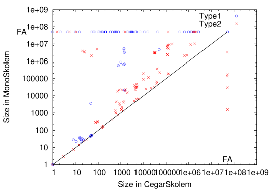
(a) Average Skolem function sizes

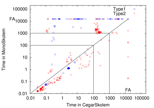
(b) Time taken (in seconds)

Figure 1: CegarSkolem vs MonoSkolem on $\textsc{TYPE-}1$ & $\textsc{TYPE-}2$ benchmarks. Topmost (rightmost) points indicate benchmarks where MonoSkolem (CegarSkolem) was unsuccessful.

Due to repeated calls to the SAT-solver, CegarSkolem takes more time than MonoSkolem on some benchmarks, but on most of them the total time taken by both algorithms is less than $100$ seconds (Figure 1(b)). Indeed, on profiling we found that CegarSkolem spent most of its time on SAT solving. On $38$ benchmarks where CegarSkolem took greater than $100$ but less than $300$ seconds, MonoSkolem performed significantly worse, taking more than $1000$ seconds. We found the degradation of MonoSkolem was due to the large sizes of Skolem functions generated (of the order of $1$ million AIG nodes) compared to those generated by CegarSkolem ($<8000$ AIG nodes). Large Skolem function sizes clearly imply more time spent in function composition and reverse-substitution.

For benchmarks where the sizes of Skolem functions generated were even larger (of the order of $10^{7}$ AIG nodes), MonoSkolem could not complete generation of all Skolem functions: for $8$ benchmarks, the memory consumed by MonoSkolem increased rapidly, resulting in memory outs; for $10$ benchmarks, it ran out of time; for an overwhelming $83$ benchmarks, it encountered integer overflows (and hence assertion failures) in the underlying ABC library. These are indicated by the topmost points (see label “FA” on the axes) in Figure 1. In contrast, CegarSkolem generated Skolem functions for almost all $(412/424)$ benchmarks. The rightmost points indicate the $12$ cases where CegarSkolem failed, of which $10$ were time-outs and $2$ were memory outs.

V-B2 CegarSkolem vs Bloqqer

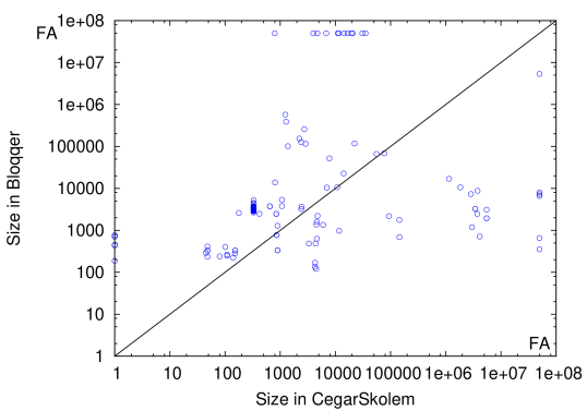
(a) Maximum size of Skolem functions

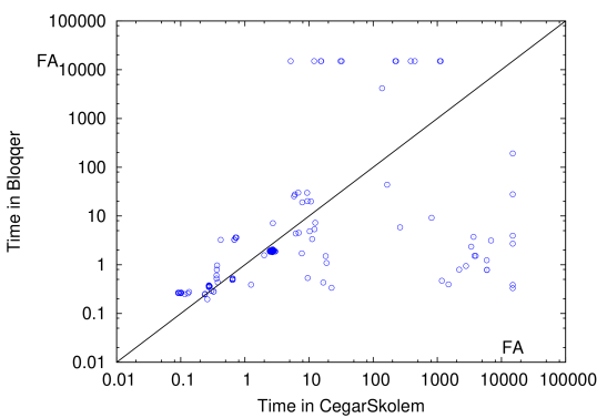
(b) Time taken (in seconds)

Figure 2: CegarSkolem vs Bloqqer on $\textsc{TYPE-}1$ benchmarks. Topmost (rightmost) points indicate benchmarks for which Bloqqer (CegarSkolem) was unsuccessful.

Of the $160$ $\textsc{TYPE-}1$ benchmarks, Bloqqer successfully generated Skolem function vectors in $148$ cases. It gave a NOT VERIFIED message for the remaining $12$ benchmarks (in less than 30 minutes). These benchmarks are indicated by the topmost points (see label “FA” on the axes) in the scatter plots of Figure 2. Of these, $8$ are large benchmarks with $1000+$ factors and variables to eliminate (overall, there are $9$ such large benchmarks). On the other hand, CegarSkolem was able to successfully generate Skolem functions on $154$ benchmarks, including the $9$ large benchmarks, on each of which it took less than $20$ minutes.

For the $142$ benchmarks for which both algorithms succeeded, we compared the times taken in Figure 2(b). As earlier, CegarSkolem took more time on many benchmarks, but there were several benchmarks, including the large benchmarks, on which Bloqqer was out-performed. We also compared the maximum sizes of Skolem functions generated in a Skolem function vector (see Figure 2(a)). We used the maximum (instead of average) size, since Tseitin encoding was needed to convert the benchmarks to qdimacs format, and this introduces many variables whose Skolem function sizes are very small, skewing the average. For a majority ($108/142$) of the benchmarks where both algorithms succeeded, the maximum sizes of Skolem functions obtained by CegarSkolem were smaller than those generated by Bloqqer. Hence, not only does CegarSkolem run faster on the large benchmarks, it also generates smaller Skolem functions on most of them.

V-B3 Discussion

For all benchmarks on which CegarSkolem timed out, we noticed that there were large subsets of factors that shared many variables in their supports. As a result, CegarSkolem could not exploit the factored representation effectively, requiring many refinements. We also noticed that for many benchmarks ($197/424$), the initial abstract Skolem functions were correct, and most of the time was spent in the SAT solver. In fact, on averaging over all benchmarks, we found that around $33\%$ of the time spent by CegarSkolem was for SAT-solving. This shows that we can leverage improvements in SAT solving technology to improve the performance of CegarSkolem.

VI Conclusion and Future Work

We presented a CEGAR algorithm for generating Skolem functions from factored propositional formulas. Our experiments show that for complex functions, our algorithm out-performs two state-of-the-art algorithms. As part of future work, we will explore integration with more efficient SAT-solvers and refinement using multiple counter-examples.

References

• [1] A. John et al. Disjunctive Decomposition Benchmarks. http://www.cse.iitb.ac.in/~supratik/tools/fmcad_2015_experiments/.
• [2] Rajeev Alur, P. Madhusudan, and Wonhong Nam. Symbolic computational techniques for solving games. STTT, 7(2):118–128, 2005.
• [3] Carlos Ansotegui, Carla P Gomes, and Bart Selman. The Achilles’ heel of QBF. In Proc. of AAAI, volume 2, pages 275–281, 2005.
• [4] Marco Benedetti. sKizzo: A Suite to Evaluate and Certify QBFs. In Proc. of CADE, pages 369–376. Springer-Verlag, 2005.
• [5] Christian Bessière and Guillaume Verger. Strategic constraint satisfaction problems. In Proc. of CP, pages 17–29, 2006.
• [6] E. Clarke, O. Grumberg, S. Jha, Y. Lu, and H. Veith. Counterexample-guided Abstraction Refinement for Symbolic Model Checking. J. ACM, 50(5):752–794, 2003.
• [7] J.-H. R. Jiang. Quantifier elimination via functional composition. In Proc. of CAV, pages 383–397. Springer, 2009.
• [8] J.-H. R. Jiang and V Balabanov. Resolution proofs and Skolem functions in QBF evaluation and applications. In Proc. of CAV, pages 149–164. Springer, 2011.
• [9] T. Jussila, A. Biere, C. Sinz, D. Kröning, and C. Wintersteiger. A First Step Towards a Unified Proof Checker for QBF. In Proc. of SAT, volume 4501 of LNCS, pages 201–214. Springer, 2007.
• [10] Berkeley Logic and Verification Group. ABC: A System for Sequential Synthesis and Verification . http://www.eecs.berkeley.edu/~alanmi/abc/.
• [11] Martina Seidl Marijn Heule and Armin Biere. Efficient Extraction of Skolem Functions from QRAT Proofs. In Proc. of FMCAD, 2014.
• [12] P. J. Ramadge and W. M. Wonham. Supervisory control of a class of discrete event processes. SIAM J. Control Optim., 25(1):206–230, 1987.
• [13] Fabio Somenzi. Binary decision diagrams. In Calculational System Design, vol. 173 of NATO Science Series F, pages 303–366. IOS Press, 1999.
• [14] S. Srivastava, S. Gulwani, and J. S. Foster. Template-based program verification and program synthesis. STTT, 15(5-6):497–518, 2013.
• [15] D. Thomas, S. Chakraborty, and P.K. Pandya. Efficient guided symbolic reachability using reachability expressions. STTT, 10(2):113–129, 2008.
• [16] A. Trivedi. Techniques in symbolic model checking. Master’s thesis, Indian Institute of Technology Bombay, Mumbai, India, 2003.
• [17] G. S. Tseitin. On the complexity of derivation in propositional calculus. Structures in Constructive Mathematics and Mathematical Logic, Part II, Seminars in Mathematics, pages 115–125, 1968.