Statics and dynamics of quasi one-dimensional Bose-Einstein condensate
in harmonic and dimple trap

Abstract

We investigate a quasi one-dimensional ${}^{87}\text{Rb}$ Bose-Einstein condensate in a harmonic trap with an additional dimple trap (dT) in the center. Within a zero-temperature Gross-Pitaevskii mean-field description we provide a one-dimensional physical intuitive model, which we solve by both a time-independent variational approach and numerical calculations. With this we obtain at first equilibrium results for the emerging condensate wave function which reveal that a dimple trap potential induces a bump or a dip in case of a red- or a blue-detuned Gaussian laser beam, respectively. Afterwards, we investigate how this dT induced bump/dip-imprint upon the condensate wave function evolves for two quench scenarios. At first we consider the generic case that the harmonic confinement is released. During the resulting time-of-flight expansion it turns out that the dT induced bump in the condensate wave function remains present, whereas the dip starts decaying after a characteristic time scale which decreases with increasing blue-detuned dT depth. Secondly, once the red- or blue-detuned dT is switched off, we find that bright shock-waves or gray/dark bi-soliton trains emerge which oscillate within the harmonic confinement with a characteristic frequency.

I Introduction

The ability to manipulate and trap atoms with laser light has had a tremendous development in many fields of physics. The very first experimental success of trapping 500 Sodium atoms for several seconds in the tight focus of a Gaussian red-detuned laser beam occurred in 1986 Chu . The physical mechanism behind such an optical dipole trap is the electric dipole interaction of the trapped polarized atoms with the intense laser light, which is far detuned from the nearest optical transition of the atoms. They are hence largely independent from magnetic sublevels of the confined atoms, in contrast to a magneto-optical trap (MOT) which can only trap atoms with a certain internal state Grimm ; Garrett . The so called dimple trap (dT) is nothing but a small tight optical dipole trap Ma ; Comparat ; Jacob . Cooling and trapping of atoms with these dT’s has a strong impact on the study of the Bose-Einstein condensates Stenger ; Stellmer , the observation of long decay times for atoms in their ground state Davidson , and the research of trapping other atomic species or molecules Weinstein .

A straightforward method for realizing a dT is to rely on the potential created by a freely propagating laser beam. The detuning of the laser frequency versus the atomic resonances determines, whether the atoms are red/blue-detuned, i.e. the laser frequency is below/above the atomic resonance frequency, respectively Grimm . The red-detuned dT was particularly used for realizing matter wave traps Ashkin ; Kurn ; Ferez in the focus of a Gaussian laser beam. On the other hand, the blue-detuned Gaussian laser beam was used in optical waveguides Xu ; Song ; Xu2 ; Noh ; Bongs ; Yin , where the creation of repulsive potentials was demonstrated by using Laguerre-Gaussian laser beam Gallatin ; Soding ; Kuga ; Kuppens ; Yin1 ; Webster . A focused or well-collimated Gaussian laser beam with a large red-detuning Metcalf or a dark hollow laser beam with a large blue-detuning Yin2 were used to form 3D optical dipole trap’s, which can be widely applied to the accurate, non-contact manipulation and control of cold atoms Barrett ; Gustavson ; Jacob .

In this paper, we will focus on studying neutral ${}^{87}\text{Rb}$ atoms within a quasi one-dimensional harmonic trap with an additional dimple trap. Experimentally, a highly elongated quasi-1D regime can be reached by tightly confining the atoms in the radial direction, effectively freezing-out the transverse dynamics Gorlitz ; Moritz ; Tolra ; Hellweg ; Kinoshita ; Chuu ; Hofferberth ; Eckart ; Pethick . It is worth mentioning that, when the transverse length scales are of the order of or less than the atomic interaction length, the one-dimensional system can only be described within the Tonks-Girardeau or within the super-Tonks-Girardeau regime Olshanii ; Petrov0 ; Bergeman , which is experimentally realizable near a confinement-induced resonance Paredes ; Kinoshita0 ; Haller . On the other hand, when the transverse confinement is larger than the atomic interaction strength, the underlying three-dimensional Gross-Pitaevskii equation (GPE) can be reduced to an effective quasi 1D model Kamchatnov . In one spatial dimension (1D) this equation is well-known, for instance, to feature bright and dark solitons for attractive and repulsive s-wave scattering lengths, respectively Radouani ; Kevrekidis ; Frantzeskakis ; Cuevas . Many experiments investigate the collision of two Bose-Einstein condensates where the celebrated matter-wave interference pattern appears Andrews or shock-waves are generated Dutton . For lower collisional energies, the repulsive interaction energy becomes significant, and the interference pattern evolves into an array of gray solitons Reinhardt ; Kivshar ; Scott ; Busch ; Ruostekoski ; Khaykovich ; Strecker ; Shomroni . Furthermore, dark solitons can be created by manipulating the condensate density using external potentials Burger ; Denschlag ; Carr ; Becker .

This work is organized as follows: In Sec. II, we start with a model which describes the dynamical evolution of a quasi-1D Bose-Einstein condensate (BEC) in a magneto-optical trap with an additional red/blue-detuned dimple trap in the center. Afterwards in Sec. III, we justify a Thomas-Fermi approximation for the condensate wave function and compare it with numerical results. With this we show that the dT induces a bump or a dip upon the condensate wave function depending on whether dT laser beam is red- or blue-detuned. Subsequently, in Sec. IV, we discuss the dynamics of the dT induced bump/dip-imprint upon the condensate wave function for two quench scenarios. After having released the trap, the resulting time-of-flight expansion shows that the dT induced imprint remains conserved for a red-detuned dT but decreases for a blue-detuned dT. Furthermore, when the initial red/blue-detuned dT is switched off, we observe the emergence of bright shock-waves or gray/dark bi-soliton trains. Finally, Sec. V summarizes our findings for the proposed quasi-1D harmonically confined BEC with an additional dimple trap in the center in view of a possible experimental realization.

II Quasi 1D model

We start with the fact that the underlying Gross-Pitaevskii equation for a condensate wave function can be formulated as the Hamilton principle of least action with the action functional

$$\mathcal{A}_{\text{3D}}=\int dt\int\mathcal{L_{\text{3D}}}\;d^{3}r,$$

where the Lagrangian density reads for three spatial dimensions

$$\mathcal{L}_{\text{3D}}= \frac{i\hbar}{2}\left[\psi^{\star}\left(\mathbf{r},t\right)\frac{\partial\psi\left(\mathbf{r},t\right)}{\partial t}-\psi\left(\mathbf{r},t\right)\frac{\partial\psi^{\star}\left(\mathbf{r},t\right)}{\partial t}\right]+\frac{\hbar^{2}}{2m_{\text{B}}}\psi^{\star}\left(\mathbf{r},t\right)\bigtriangleup\psi\left(\mathbf{r},t\right)-V(\mathbf{r})\psi^{\star}\left(\mathbf{r},t\right)\psi\left(\mathbf{r},t\right)$$

$$-U_{\textrm{dT}}^{\textrm{3D}}\left(\mathbf{r}\right)\psi^{\star}\left(\mathbf{r},t\right)\psi\left(\mathbf{r},t\right)-\frac{G_{\text{B}}^{\text{3D}}}{2}\parallel\psi\left(\mathbf{r},t\right)\parallel^{4}\,.$$ (1)

Here $\psi\left(\mathbf{r},t\right)$ describes the BEC wave function with the coordinates $\mathbf{r}=\left(x,\;y,\;z\right)$ and the two-particle interaction strength reads $G_{\text{B}}^{\text{3D}}=N_{\text{B}}4\pi\hbar^{2}a_{\text{B}}/m_{\text{B}}$, where $N_{\text{B}}$ denotes the number of bosonic atoms. In case of ${}^{87}\text{Rb}$ atoms, the s-wave scattering length is $a_{\text{B}}=94.7~{}{\rm{a}_{0}}$ with the Bohr radius ${\rm{a}_{0}}$. We assume that the bosons are confined by a harmonic potential with an additional dT potential in the center.

For instance, a MOT yields a harmonic confinement $V\left(\mathbf{r}\right)=m_{\text{B}}\omega_{\text{z}}^{2}z^{2}/2+m_{\text{B}}\omega_{\text{r}}^{2}\left(x^{2}+y^{2}\right)/2$, which has rotational symmetry with respect to the $z$-axis. In the following, we consider the experimentally realistic trap frequencies $\omega_{\text{r}}=2\pi\times 160\,\textrm{Hz}\gg\omega_{\text{z}}=2\pi\times 6.8\,\textrm{Hz}$ Garrett , so we have a cigar-shaped condensate, where the oscillator lengths amount to the values $l_{\text{r}}=0.84\,\mu\textrm{m}\ll l_{\text{z}}=4.12\,\mu\textrm{m}$.

An additional three-dimensional narrow Gaussian laser beam polarizes the neutral atoms and, thus, yields the dT potential $U_{\textrm{dT}}^{\textrm{3D}}=U_{\textrm{0}}\textrm{I}\left(\mathbf{r}\right)$. Within the rotating-wave approximation its amplitude $U_{\textrm{0}}$ is given by Milonni ; Saleh ; Allen ; Scully

$$U_{\textrm{0}} =\frac{3\pi c^{2}\Gamma}{2\omega_{\textrm{A}}^{3}\Delta}\,.$$ (2)

Here $\Gamma=\left|<e|{\bf d}|g>\right|^{2}\omega_{\textrm{A}}^{3}/\left(3\pi\epsilon_{0}\hbar c^{3}\right)$ denotes the damping rate due to energy loss via radiation, which is determined by the dipole matrix element between ground $g$ and excited state $e$. Furthermore, $\Delta=\omega-\omega_{\textrm{A}}$ represents the detuning of the laser, where $\omega$ is the laser frequency and $\omega_{\textrm{A}}$ stands for the frequency of the D₁- or D₂-line of ${}^{87}\text{Rb}$ atoms, which are the transitions $5^{2}S{}_{1/2}\rightarrow 5^{2}P{}_{1/2}$ or $5^{2}S{}_{1/2}\rightarrow 5^{2}P{}_{3/2}$ with the wave lengths $\lambda_{\textrm{D}1}=794.76\,\textrm{nm}$ and $\lambda_{\textrm{D}2}=780.03\,\textrm{nm}$, respectively. The intensity profile of the Gaussian laser beam, which is assumed to move in $y$-direction, is determined via

$$\textrm{I}\left(\mathbf{r}\right)=\frac{2P}{\pi W_{\text{x}}\left(y\right)W_{\text{z}}\left(y\right)}e^{-\left[\frac{2x^{2}}{W_{\text{x}}^{2}\left(y\right)}+\frac{2z^{2}}{W_{\text{z}}^{2}\left(y\right)}\right]}\,,$$ (3)

where $P$ denotes its power. Furthermore, $W_{\text{x/z}}(y)=W_{\text{0x/z}}\sqrt{1+y^{2}/y_{\text{Rx/z}}^{2}}$ defines the beam radius in $x$- and $z$-direction, where the intensity decreases to $1/e^{2}$ of its peak value, and the Rayleigh lengths $y_{\text{Rx/z}}=\pi W_{\text{0x/z}}/\lambda$ with wave length $\lambda=2\pi c/\omega$ define the distances where the beam radius increases by a factor of $\sqrt{2}$ Saleh . We use for the Gaussian laser beam width along the $x$-axis $W_{\text{0x}}=1.1\,\mu\textrm{m}$ and along the $z$-axis $W_{\text{0z}}=3.2\,\mu\textrm{m}$, which are about ten times smaller than the corresponding ones used in Ref. Garrett . The corresponding Rayleigh lengths for the red-detuned laser light with $\lambda=840\,\textrm{nm}$ Garrett yield $y_{\text{Rx}}=4.526\,\mu\textrm{m}$ and $y_{\text{Rz}}=38.29\,\mu\textrm{m}$ and for the blue-detuned laser light with $\lambda=772\,\textrm{nm}$ Xu-1 we get $y_{\text{Rx}}=4.92\,\mu\textrm{m}$ and $y_{\text{Rz}}=41.6\,\mu\textrm{m}$. Due to the fact $y_{\text{Rx}/\text{z}}\gg l_{\text{r}}$, we can approximate the widths of the beam in $x$- and $z$-direction according to $W_{\text{x}/\text{z}}(y)\approx W_{0\text{x}/\text{z}}$. This simplifies the dimple trap to

$$U_{\textrm{dT}}^{\textrm{3D}}\left(\mathbf{r}\right) =\frac{2U_{0}P}{\pi W_{0\text{x}}W_{0\text{z}}}e^{-\left(\frac{2x^{2}}{W_{\text{0x}}^{2}}+\frac{2z^{2}}{W_{\text{0z}}^{2}}\right)}.$$ (4)

As the MOT provides a quasi one-dimensional setting due to $a_{\text{B}}\ll l_{\text{r}}\ll l_{\text{z}}$, we can follow Ref. Kamchatnov , and decompose the BEC wave-function $\psi(\mathbf{r},t)=\psi(z,t)\phi({\bf r}_{\perp},t)$ with ${\bf r}_{\perp}=\left(x,\;y\right)$ and

$$\phi({\bf r}_{\perp},t) = \frac{e^{-\frac{x^{2}+y^{2}}{2l_{\text{r}}^{2}}}}{\sqrt{\pi}l_{\text{r}}}e^{-i\omega_{\text{r}}t}\,.$$ (5)

Subsequently, we integrate out the two transversal dimensions of the three-dimensional Lagrangian according to

$$\mathcal{L}_{\text{1D}}=\int_{-\infty}^{\infty}\int_{-\infty}^{\infty}\mathcal{L}_{\text{3D}}\;dxdy.$$ (6)

After a straight-forward calculation the resulting quasi one-dimensional Lagrangian reads

$$\mathcal{L}_{\text{1D}}= \frac{i\hbar}{2}\left[\psi^{\star}\left(z,t\right)\frac{\partial\psi\left(z,t\right)}{\partial t}-\psi\left(z,t\right)\frac{\partial\psi^{\star}\left(z,t\right)}{\partial t}\right]+\frac{\hbar^{2}}{2m_{\text{B}}}\psi^{\star}\left(z,t\right)\frac{\partial^{2}\psi\left(z,t\right)}{\partial z^{2}}-V(z)\psi^{\star}\left(z,t\right)\psi\left(z,t\right)$$

$$-\textrm{U}e^{-\frac{2z^{2}}{W_{\text{0z}}^{2}}}\psi^{\star}\left(z,t\right)\psi\left(z,t\right)-\frac{G_{\text{B}}}{2}\parallel\psi\left(z,t\right)\parallel^{4},$$ (7)

where $V\left(z\right)=m_{\text{B}}\omega_{z}^{2}z^{2}/2$ represents an effective one-dimensional harmonic potential from the MOT, and the one-dimensional two-particle interaction strength is

$$G_{\text{B}}=2N_{\text{B}}a_{\text{B}}\hbar\omega_{\text{r}}\,.$$ (8)

Furthermore, the one-dimensional dT depth turns out to be

$$\textrm{U}=\frac{2U_{0}P}{\pi W_{\text{0z}}\sqrt{W_{\text{0x}}^{2}+2l_{\text{r}}^{2}}}\,,$$ (9)

which depends on the power of the laser beam $P$ as well as via (2) and the detuning $\Delta=\omega-\omega_{\textrm{A}}$ on the laser wave length $\lambda$. Note that the latter not only changes the absolute value of the dT depth but also its sign via the detuning $\Delta$. For red detuning, i.e. when the laser frequency is smaller than the atomic frequency, the dT is negative and atoms are sucked into the dT potential. In the opposite case of blue detuning the atoms are repelled from the dT potential. Thus, the dT induces an imprint on the BEC wave function, which can be either a bump for red detuning or a dip for blue detuning. In the following we will analyze this interesting effect in more detail.

To this end we consider the 1D action

$$\mathcal{A}_{\text{1D}}= \int_{-\infty}^{\infty}\int_{-\infty}^{\infty}\mathcal{L}_{\text{1D}}\left(\psi^{\star}\left(z,t\right),\frac{\partial\psi^{\star}\left(z,t\right)}{\partial t},\frac{\partial\psi^{\star}\left(z,t\right)}{\partial z};\psi\left(z,t\right),\frac{\partial\psi\left(z,t\right)}{\partial t},\frac{\partial\psi\left(z,t\right)}{\partial z}\right)dzdt$$ (10)

and determine the time dependent one-dimensional Gross-Pitaevskii equation (1DGPE) according to the Euler-Lagrangian equation

$$\frac{\delta\mathcal{A}_{\text{1D}}\left[\psi^{\star},\psi\right]}{\delta\psi^{\star}\left(z,t\right)}= \frac{\partial\mathcal{L}_{\text{1D}}}{\partial\psi^{\star}\left(z,t\right)}-\frac{\partial}{\partial z}\frac{\partial\mathcal{L}_{\text{1D}}}{\partial\frac{\partial\psi^{\star}\left(z,t\right)}{\partial z}}-\frac{\partial}{\partial t}\frac{\partial\mathcal{L}_{\text{1D}}}{\partial\frac{\partial\psi^{\star}\left(z,t\right)}{\partial t}}=0.$$ (11)

By using the one-dimensional Lagrangian density (7) the 1DGPE reads

$$i\hbar\frac{\partial}{\partial t}\psi(z,t)=\left\{-\frac{\hbar^{2}}{2m_{B}}\frac{\partial^{2}}{\partial z^{2}}+\frac{m_{\text{B}}\omega_{z}^{2}}{2}z^{2}+\textrm{U}e^{-\frac{2z^{2}}{W_{\text{0z}}^{2}}}+G_{\text{B}}\parallel\psi(z,t)\parallel^{2}\right\}\psi(z,t).$$ (12)

On the right-hand side the first term represents the kinetic energy of the atoms with mass $m_{\text{B}}$, the second term describes the harmonic MOT potential, the third term stands for the dT potential, and the last term represents the two-particle interaction. In order to make Eq. (12) dimensionless, we introduce the dimensionless time as $\tilde{t}=\omega_{\text{z}}t$, the dimensionless coordinate $\tilde{z}=z/l_{\text{z}}$, and the dimensionless wave function $\tilde{\psi}=\psi/\sqrt{l_{\text{z}}}$. With this Eq. (12) can be written in the form

$$i\frac{\partial}{\partial\tilde{t}}\tilde{\psi}\left(\tilde{z},\tilde{t}\right) =\left\{-\frac{1}{2}\frac{\partial^{2}}{\partial\tilde{z}^{2}}+\frac{1}{2}\tilde{z}^{2}+\tilde{\textrm{U}}e^{-\frac{\tilde{z}^{2}}{\tilde{\alpha}^{2}}}+\tilde{G}_{\text{B}}\parallel\tilde{\psi}\left(\tilde{z},\tilde{t}\right)\parallel^{2}\right\}\tilde{\psi}\left(\tilde{z},\tilde{t}\right),$$ (13)

where we have $\tilde{G}_{\text{B}}=2N_{\text{B}}\omega_{\text{r}}a_{\text{B}}/\left(\omega_{\text{z}}l_{\text{z}}\right)$ and $\tilde{\textrm{U}}=\textrm{U}/\left(\hbar\omega_{\text{z}}\right)$. For the above mentioned experimental parameters and $N_{\text{B}}=20\times 10^{4}$ atoms of ${}^{87}\text{Rb}$, we obtain the dimensionless couplings constant $\tilde{G}_{\text{B}}=11435.9$. Furthermore, the typical dT depth $\left|\textrm{U}\right|/k_{\text{B}}=210\,\textrm{nK}$ yields the dimensionless value $\left|\tilde{U}\right|=643.83$, and $\tilde{\alpha}=W_{\text{0z}}/\left(\sqrt{2}l_{\text{z}}\right)=0.548$ represents the ratio of the width of the dT potential along the $z$-axis and the longitudinal harmonic oscillator length. From here on, we will drop all tildes for simplicity.

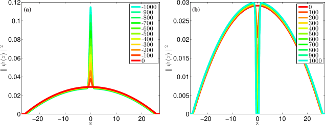
Figure 1: (Color online) Numerical density profile of BEC for the experimental coupling constant value $G_{\text{B}}=11435.9$ and for the dT depth U which increases from top to bottom according to the inlets. For a) negative values of U, the bump in the condensate wave function decreases, whereas for b) positive values the corresponding dip increases.

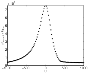
Figure 2: (Color online) Ratio $E_{\text{int,pot}}/E_{\text{kin}}$ versus U from solving 1DGPE (13).

III dT induced bump/dip-Imprint Upon Stationary Condensate Wave Function

In order to determine the dT induced imprint on the condensate wave function in equilibrium, we solve the 1DGPE (13) in imaginary time numerically by using the split-operator method Javanainen ; Vudragovic . In this way we find that the dT-imprint leads to a bump/hole in the BEC density at the trap center for negative/positive values of U as shown in Fig. 1. For stronger red-detuned dT depth values the bump increases further, but for stronger blue-detuned dT the dip in the BEC density gets deeper and deeper until no more BEC atoms remain in the trap center. After this qualitative overview on the numerical results, we now work out an analytic approach for describing this red/blue-detuned dT induced bump/dip on the BEC density in a more quantitative way. To this end we present two arguments why the seminal Thomas-Fermi (TF) approximation is also applicable in our context.

At first we provide a rough estimate in the case of an absent dT, i.e. U$=0$, so the BEC density is characterized by the TF profile $\psi\left(z\right)=\sqrt{\left(\mu-z^{2}/2\right)/G_{\text{B}}}\Theta\left(\mu-z^{2}/2\right)$, where the Heaviside function $\Theta$ prevents the density to become negative. Thus, the Tomas-Fermi radius $\sqrt{2\mu}$ follows from the dimensionless chemical potential $\mu$, which is determined by normalization to be $\mu=\frac{1}{2}\left(\frac{3}{2}\right)^{2/3}(G_{\text{B}})^{2/3}$. As the red/blue-detuned dT is supposed to be inserted at the trap center, we then calculate the dimensionless BEC coherence length $\xi$ at the trap center. It is defined by comparing the kinetic energy $1/2\xi^{2}$ with the interaction energy in the trap center, which is given by $\mu$. For the above mentioned experimental parameters this yields the dimensionless BEC coherence length $\xi=0.038$, which is about 14.4 times smaller than the dT width $\alpha=0.548$. This indicates that the dT induced imprint upon the BEC wave-function occurs on a length scale which is much larger than its coherence length, so the TF approximation seems to be reasonable even in the presence of the red/blue-detuned dT.

In view of a more quantitative justification for the applicability of the Thomas-Fermi approximation, Fig. 2 presents the numerical result how the ratio of the sum of interaction and potential energy $E_{\textrm{{\rm int,pot}}}$ versus the kinetic energy $E_{{\rm kin}}$ of the condensate wave function changes with increasing or decreasing the red/blue-detuned dT depth U. The maximal value of this energy ratio occurs for U$=0$ and amounts to 7.5$\times 10^{4}$, which is of the order of the number of particles. Furthermore, we read off that the inequality $E_{\textrm{{\rm int,pot}}}/E_{\textrm{{\rm kin}}}\gg 1$ holds within the whole region of interest for U, so the TF approximation is there, indeed, valid.

Therefore, we investigate in the following the TF approximation in more detail for non-zero red/blue-detuned dT depth U. To this end we use for the condensate wave function the ansatz $\psi(z,t)=\psi(z)e^{-i\mu t}$, insert it into the 1DGPE (13), and neglect the kinetic energy term, which yields the density profile

$$\psi\left(z\right)=\sqrt{\frac{1}{G_{\text{B}}}\left(\mu-\frac{z^{2}}{2}-\textrm{U}e^{-\frac{z^{2}}{\alpha^{2}}}\right)}\Theta\left(\mu-\frac{z^{2}}{2}-\textrm{U}e^{-\frac{z^{2}}{\alpha^{2}}}\right)\,.$$ (14)

In view of the normalization $\intop_{-\infty}^{+\infty}\parallel\psi\left(z\right)\parallel^{2}dz=1$, which fixes the chemical potential $\mu$, we have to determine the Thomas-Fermi radii $R_{\text{TF}}$ from the condition that the condensate wave function vanishes:

$$\mu=\frac{R_{\text{TF}}^{2}}{2}+\textrm{U}e^{-\frac{R_{\text{TF}}^{2}}{\alpha^{2}}}.$$ (15)

As can be read off from Fig. 1 the number of solutions of Eq. (15) changes for increasing dT depth at a critical value $\textrm{U}_{\text{c}}$, which follows from solving the implicit equation

$$\textrm{U}_{\text{c}}=\frac{1}{2}\left(\frac{3}{2}\right)^{\frac{2}{3}}(G_{\text{B}}+\sqrt{\pi}\alpha\textrm{U}_{\text{c}})^{\frac{2}{3}}\,.$$ (16)

This yields the result $\textrm{U}_{\text{c}}\approx 339.5$ for the experimental coupling constant $G_{\text{B}}=11435.9$, which compares well with the value $\textrm{U}_{\text{c}}\approx 342$ determined from solving 1DGPE (13). In the case that U is smaller than $\textrm{U}_{\text{c}}$ Eq. (15) defines only the cloud radius $R_{\text{TF1}}$. But for the case $\textrm{U}>\textrm{U}_{\text{c}}$ the dT drills a hole in the center of the ${}^{87}\text{Rb}$ condensate, so it fragments into two parts. Thus, we have then apart from the outer cloud radius $R_{\text{TF1}}$ also an inner cloud radius $R_{\text{TF2}}$. With this the normalization condition $2\intop_{R_{\text{TF2}}}^{R_{\text{TF1}}}\parallel\psi\left(z\right)\parallel^{2}dz=1$ yields

$$\mu\left(R_{\text{TF1}}-R_{\text{TF2}}\right)-\frac{1}{6}\left(R_{\text{TF1}}^{3}-R_{\text{TF2}}^{3}\right)=\frac{G_{\text{B}}}{2}+\frac{\sqrt{\pi}\alpha\textrm{U}}{2}\left[\text{Erf}\left(\frac{R_{\text{TF1}}}{\alpha}\right)-\text{Erf}\left(\frac{R_{\text{TF2}}}{\alpha}\right)\right]\,,$$ (17)

where $\text{Erf}(y)=\frac{2}{\sqrt{\pi}}\int_{0}^{y}e^{-x^{2}}dx$ denotes the error function. In case of $\textrm{U}\leq\textrm{U}_{\text{c}}$ the inner cloud radius $R_{\text{TF2}}$ vanishes and the cloud radius is approximated via $R_{\text{TF1}}\approx\sqrt{2\mu}$ due to Eq. (15) as it is much larger than the dimple trap width $\alpha$. Thus, the chemical potential is determined explicitly from

$$\mu\approx\frac{1}{2}\left(\frac{3}{2}\right)^{2/3}\left(G_{\text{B}}+\sqrt{\pi}\alpha\textrm{U}\right)^{2/3}\,,\quad\textrm{U}\leq\textrm{U}_{\text{c}}\,.$$ (18)

Provided that $\textrm{U}\geq\textrm{U}_{\text{c}}$, the inner cloud radius $R_{\text{TF2}}$ has to be taken into account according to Fig. 1 and, due to the fact that $R_{\text{TF2}}^{2}\ll\textrm{U}$, we get from Eq. (15) the approximation $\mu\approx\textrm{U}e^{-\frac{R_{\text{TF2}}^{2}}{\alpha^{2}}}$, which reduces to

$$R_{\text{TF2}}\approx\alpha\sqrt{\log\left(\frac{\textrm{U}}{\mu}\right)}.$$ (19)

Thus, we conclude that $R_{\text{TF2}}$ vanishes, indeed, at $\textrm{U}_{\text{c}}$ according to Eq. (16) and Eq. (18). With this we obtain from Eq. (17) that the chemical potential follows from solving

$$3\left[\sqrt{\pi}\alpha\textrm{U}+G_{\text{B}}+2\alpha\mu\sqrt{\log\left(\frac{\textrm{U}}{\mu}\right)}\right]\approx 3\sqrt{\pi}\alpha\textrm{U}\text{Erf}\left(\sqrt{\log\left(\frac{\textrm{U}}{\mu}\right)}\right)+\alpha^{3}\log^{\frac{3}{2}}\left(\frac{\textrm{U}}{\mu}\right)+4\sqrt{2}\mu^{3/2}\,,\,\textrm{U}\geq\textrm{U}_{\text{c}}\,.$$ (20)

Figure 3 shows the resulting outer and inner Thomas-Fermi radius as a function of the dT depth U. We read off that $R_{\text{TF1}}\approx\sqrt{2\mu}$ remains approximately constant for $\textrm{U}\geq\textrm{U}_{\text{c}}$, so we conclude that the chemical potential $\mu$ is locked to its critical value $\mu_{c}\approx\textrm{U}_{\text{c}}=339.5$. Furthermore, we note that the inner Thomas-Fermi radius $R_{\text{TF2}}$ increases up to about $5.4\alpha$ for the considered range of U.

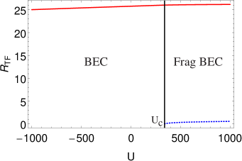
Figure 3: (Color online) Outer Thomas-Fermi radius $R_{\text{TF1}}$ (red solid) and inner Thomas-Fermi radius $R_{\text{TF2}}$ (blue dashed) versus dimple trap depth U. BEC fragments into two parts above $\textrm{U}_{\text{c}}\approx 339.5$.

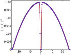
Figure 4: (Color online) Condensate density for $\textrm{U}=1000$ from solving 1DGPE (13) in imaginary time numerically (red) and from TF approximation (14) (blue-circles).

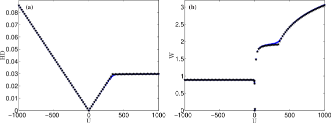
Figure 5: (Color online) a) Height/depth and b) width of the dT induced bump/dip according to Eqs. (25)–(27), versus the red/blue-detuned dT depth U for the experimental BEC coupling constant $G_{\text{B}}=11435.9$ calculated numerically by solving 1DGPE (13) in imaginary time (blue circles) and analytically (black stars) from the TF condensate wave function (14).

Figure 4 compares the resulting TF condensate wave function (14) with a numerical solution of the 1DGPE (13) in imaginary time at U$=1000$ and we read off that both agree quite well. Thus, our TF approximation describes the equilibrium properties of the condensate wave function in the presence of the red/blue-detuned dT even quantitatively correct. In view of a more detailed comparison, we characterize the red/blue-detuned dT induced imprint upon the condensate wave function $\psi(z)$ by the following two quantities. The first one is the hight/depth (HD) of the dT induced imprint

$$\begin{array}[]{r@{}l@{\,}l}\text{HD}=\left\{\begin{array}[]{r@{}l@{\,}l}\parallel\psi\left(0\right)\parallel_{\textrm{U}}^{2}-\parallel\psi\left(0\right)\parallel_{\textrm{U}=0}^{2}\qquad\textrm{U}\leq 0\\ \\ \text{Max}\left(\parallel\psi\left(z\right)\parallel_{\textrm{U}}^{2}\right)-\parallel\psi\left(0\right)\parallel_{\textrm{U}}^{2}\qquad\textrm{U}\geq 0\end{array}\right.\end{array}$$ (25)

and the second one is the red/blue-detuned dT induced imprint width W, which we define as follows. For $\textrm{U}\leq 0$ we use the full width half maximum

$$\parallel\psi\left(\text{W/2}\right)\parallel_{\textrm{U}}^{2}=\left(\parallel\psi\left(0\right)\parallel_{\textrm{U}}^{2}+\parallel\psi\left(0\right)\parallel_{\textrm{U}=0}^{2}\right)/2\qquad\textrm{U}\leq 0\,,$$ (26)

whereas for $\textrm{U}>0$ we define the equivalent width Carroll :

$$\text{W}=\left(2I_{\text{0}}z_{\text{Max}}-\intop_{-z_{\text{Max}}}^{z_{\text{Max}}}\parallel\psi\left(z\right)\parallel_{\textrm{U}}^{2}dz\right)/\left(I_{\text{0}}-\parallel\psi\left(0\right)\parallel_{\textrm{U}}^{2}\right)\qquad\textrm{U}>0\,,$$ (27)

where we have $I_{\text{0}}=\text{Max}\left(\parallel\psi\left(z\right)\parallel_{\textrm{U}}^{2}\right)$. Figure 5 a) shows the red/blue-detuned dT induced imprint height/depth as a function of U. At first, we read off that for $\textrm{U}=0$, i.e. when we have not switched on the dT, bump/dip vanishes. Furthermore, in the range $\textrm{U}\leq\textrm{U}_{\text{c}}$ we observe that height/depth of the dT induced imprint bump/dip changes linearly with U according to

$$\text{HD}\approx\frac{|\textrm{U}|}{G_{\text{B}}}\,.$$ (28)

In case of $\textrm{U}>\textrm{U}_{\text{c}}$ height/depth of the dT induced imprint has approximately the constant value $\text{HDc}=\textrm{U}_{\text{c}}/G_{\text{B}}\approx 0.029$ as follows from the TF wave function (14) and the above mentioned locking of the chemical potential to its critical value. Note that this constant value only slightly deviates from the corresponding numerical value $\text{HDc}=0.03$.

Correspondingly, Figure 5 b) depicts the dimple trap induced width W as a function of U. From our TF approximation we obtain for the width transcendental formulas, which read in case of $\textrm{U}\leq 0$

$$\frac{\text{W}^{2}}{4}+2\textrm{U}e^{-\frac{\text{W}^{2}}{4\alpha^{2}}}-\textrm{U}+\frac{1}{2}\left(\frac{3}{2}\right)^{2/3}\left[\left(G_{\text{B}}\right)^{2/3}-\left(G_{\text{B}}+\sqrt{\pi}\alpha\textrm{U}\right)^{2/3}\right]=0\,,$$ (29)

and for $\textrm{U}>\alpha^{2}/2$

$$\text{W}=\frac{2\alpha^{3}\sqrt{\log\left(\frac{2\textrm{U}}{\alpha^{2}}\right)}\left[2\log\left(\frac{2\textrm{U}}{\alpha^{2}}\right)+3\right]-6\sqrt{\pi}\alpha\textrm{U}\text{Erf}\left(\sqrt{\log\left(\frac{2\textrm{U}}{\alpha^{2}}\right)}\right)}{3\left[\alpha^{2}+\alpha^{2}\log\left(\frac{2\textrm{U}}{\alpha^{2}}\right)-2\textrm{U}\right]}\,.$$ (30)

As shown in Fig. 5 b), for an increasing red-detuned dT depth, the width remains approximately constant, but just before $\textrm{U}=0$ starts to decrease to zero. For a blue-detuned dT the width of the dip continuously increases with an intermediate plateau at $\textrm{U}_{\text{c}}$ with the value $\text{Wc}\approx 1.91$, which agrees well with the numerically obtained one $\text{Wc}\approx 1.99$.

IV Dimple trap induced imprint upon Condensate Dynamics

In an experiment, any dT induced bump/dip upon the condensate wave function could only be detected dynamically. Thus, it is of high interest to study theoretically whether the dT induced bump/dip imprint, which we have found and analyzed for the stationary case in the previous section, remains present also during the dynamical evolution of the condensate wave function. To this end we investigate two quench scenarios numerically in more detail. The first one is the standard time-of-flight (TOF) expansion after having switched off the harmonic trap when the amplitude of the red/blue-detuned dT is still present. In the second case we consider the inverted situation that the red/blue-detuned dT is suddenly switched off within a remaining harmonic confinement, which turns out to give rise to the emergence of bright shock-waves or bi-solitons trains, respectively.

IV.1 Time-of-Flight Expansion

Time-of-flight (TOF) absorption pictures represent an important diagnostic tool to analyze dilute quantum gases since the field’s inception. By suddenly turning off the magnetic trap, the atom cloud expands with a dynamics which is determined by both the momentum distribution of the atoms at the instance, when the confining potential is switched off, and by inter-atomic interactions Mewes ; Inouye . We have investigated the time-of-flight expansion dynamics of the BEC with the dT by solving numerically the 1DGPE (13) and analyzing the resulting evolution of the condensate wave function. It turns out that, despite the continuous broadening of the condensate density, its dT induced imprint remains qualitatively preserved both for red and blue-detuned dT. Therefore, we focus a more quantitative discussion upon the dynamics of the corresponding dT induced imprint height/depth and width.

For a red-detuned dT, it turns out that the bump height even remains constant in time. This is shown explicitly in Fig. 6 a), which roughly preserves its initial value at $t=0$. In case of the bump width, we even find that no significant changes do occur neither in time nor for varying U, therefore we do not present a corresponding figure. Note that the latter finding originates from Fig. 5 b), where the width is shown to be roughly constant for all dT depths.

Instead, in case of a blue-detuned dT, the dip decays after a characteristic time scale as shown in Fig. 6 b). The inlet reveals that the dip relaxes with a shorter time scale for increasing blue-detuned dT depth U. In addition, we read off from Fig. 7 that, at the beginning of TOF, the dT induced imprint width remains at first constant and then increases gradually. This change of W occurs on the scale of the relaxation time of HD, which is depicted in Fig. 6 b).

Figure 6: (Color online) Height/depth of the dT induced imprint after having released the harmonic trap versus time for a) increasing negative and b) decreasing positive values of dT depth U from top to bottom. Inlet: relaxation time $t_{\text{rel}}$ decreases with increasing U.

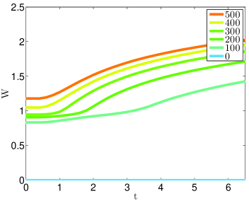
Figure 7: (Color online) Width of the dT induced imprint after having released the trap versus time for decreasing positive values of dT depth U from top to bottom.

IV.2 Wave Packets Versus Solitons

Due to their quantum coherence, BECs exhibit rich and complex dynamic patterns, which range from the celebrated matter-wave interference of two colliding condensates Andrews ; Dutton over Faraday waves engels ; balaz to the particle-like excitations of solitons Reinhardt ; Kivshar ; Scott ; Busch ; Ruostekoski ; Becker ; Shomroni . For our 1D model of a BEC with a harmonic and a dimple trap in the center, we investigated the dynamics of the condensate wave function which emerges after having switched off the dT. To this end, Fig. 8 depicts the resulting profile of density $n=|\psi|^{2}$ and phase $\phi=\tan^{-1}\left(\psi_{{\rm Re}}/\psi_{{\rm Im}}\right)$ of the condensate wave function $\psi$ at different instants of time. Both for an initial red- and blue-detuned dT, we observe that two excitations of the condensate are created at the dT position, which travel in opposite direction with the same center-of-mass speed, are reflected at the trap boundaries and then collide at the dT position. Furthermore, we find that these excitations qualitatively preserve their shape despite the collision and that the BEC wave function reveals characteristic phase slips between $-\pi/2$ and $\pi/2$. All these findings are not yet conclusive to decide whether these excitations represent wave packets in the absence of dispersion or solitons. Therefore, we investigate their dynamics in more detail, by determining their center-of-mass motion via

$$\bar{z}_{{\rm{L,R}}}\left(t\right)=\frac{\int_{-\infty,0}^{0,\infty}z\left(\parallel\psi\left(z,t\right)\parallel_{\text{U}}^{2}-\parallel\psi\left(z,t\right)\parallel_{\text{U}=0}^{2}\right)dz}{\int_{-\infty,0}^{0,\infty}\left(\parallel\psi\left(z,t\right)\parallel_{\text{U}}^{2}-\parallel\psi\left(z,t\right)\parallel_{\text{U}=0}^{2}\right)dz}\,,$$ (31)

which are plotted in Fig. 9. Note that the mean positions $\bar{z}_{{\rm{L}}}$ and $\bar{z}_{{\rm{R}}}$ of the excitations are uncertain in the region where they collide. Nevertheless Fig. 9 demonstrates that the excitations oscillate with the frequency $\Omega=2\pi\times 4.87~{}{\rm Hz}$ irrespective of sign and size of U. As we have assumed the trap frequency $\omega_{{\rm z}}=2\pi\times 6.8~{}{\rm Hz}$, we obtain the ratio $\Omega/\omega_{{\rm z}}\approx 0.72$, which is quite close to $\Omega/\omega_{{\rm z}}=1/\sqrt{2}\approx 0.707$.

Despite these similarities of the cases of an initial red and blue-detuned dT, we observe one significant difference. Whereas the oscillation amplitudes of the excitations do not depend on the value of the initial $\textrm{U}<0$ according to Fig. 9 a), we find decreasing oscillation amplitudes of the excitations with increasing the initial $\textrm{U}>0$ in Fig. 9 b). Such an amplitude dependence on the initial condition is characteristic for gray/dark solitons according to Ref. Busch . This particle-like interpretation of the excitations agrees with the other theoretical prediction of Ref. Busch that gray/dark solitons oscillate in a harmonic confinement with the frequency $\Omega/\omega_{{\rm z}}=1/\sqrt{2}$, which was already confirmed in the Hamburg experiment of Ref. Becker and is also seen in Fig. 9.

Conversely, for an initial red-detuned dT the excitations can not be identified with bright solitons as the dynamics is governed by a GPE with a repulsive two-particle interaction. Here the excitations have to be interpreted as wave packets which move without any dispersion as follows from a Bogoliubov dispersion relation and the smallness of the coherence length. Thus, for $\textrm{U}<0$ the excitations propagate like sound waves in the BEC andrews1 and, within a TF approximation, their center-of-mass motion is described by the evolution equation Damski1

$$\frac{dz(t)}{dt}=\sqrt{\mu-\frac{z^{2}(t)}{2}}\,.$$ (32)

Solving (32) with the initial condition $z(0)=0$ yields the result $z(t)=\sqrt{2\mu}\sin t/\sqrt{2}$. Thus, we read off that the oscillation amplitude coincides with the TF radius and that the dimensionless oscillation frequency turns out to be $\Omega=1/\sqrt{2}$ in agreement with Fig. 9 a).

Thus, we conclude that switching off the red/blue-detuned dT leads to physically different situations. For an initial red-detuned dT, we generate wave packets which correspond to white shock waves Damski2 , whereas for the corresponding blue-detuned case bi-soliton trains emerge Reinhardt ; Strecker ; Khawaja , due to the collision of the two fragmented parts of the condensate. Note that it can be shown in our system that gray bi-solitons trains are generated for a partially fragmented BEC, i.e. $\textrm{U}<\textrm{U}_{\text{c}}$. On the other hand the dark bi-solitons trains turn out to be only generated for $\textrm{U}\geq\textrm{U}_{\text{c}}$, where the BEC is well fragmented into two parts equilibrium.

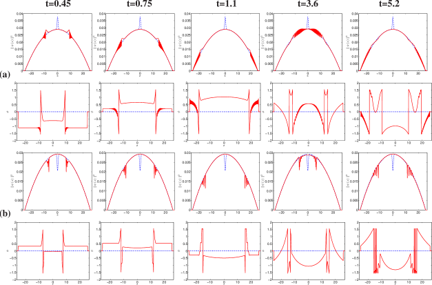
Figure 8: (Color online) Density (phase) profile of BEC after having switched off the red/blue-detuned dT: in blue-dashed line at $t$=0, and in red-solid line at $t$=0.45 ($1^{{\rm st}}$ column), $t$=0.75 ($2^{{\rm nd}}$ column), $t$=1.1 ($3^{{\rm rd}}$ column), $t$=3.6 ($4^{{\rm th}}$ column), and $t$=5.2 ($5^{{\rm th}}$ column) for (a) $U$=-100 and (b) $U$=100.

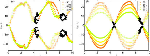
Figure 9: (Color online) Center of mass positions of excitations $\bar{z}_{{\rm L}}$ (filled circles) and $\bar{z}_{{\rm R}}$ (empty circles) according to Eq. (31) versus time after having switched off the dT with increasing absolute value of the depth $|\textrm{U}|$ from top to bottom, for a) red-detuning and b) blue-detuning. Black filled circles represent the region of colliding excitations, where mean positions are not perfectly detectable.

V Summary and Conclusion

In the present work we studied within a quasi 1D model both analytically and numerically how a dimple trap in the center of a harmonically trapped BEC affects the condensate wave function. At first, we showed for the equilibrium properties of the system that the Thomas-Fermi approximation agrees quantitatively with numerical solutions of the underlying 1D Gross-Pitaevskii equation. For an increasing red-detuned dT depth, it turns out for the induced bump that the height decreases linearly, whereas the width remains approximately constant. In contrast to that we found for an increasing blue-detuned dT that depth and width of the induced dip initially increase. Beyond a critical value $\textrm{U}_{\text{c}}$, the BEC even fragments into two parts and, if U is increased beyond $\textrm{U}_{\text{c}}$, the dT induced imprint yields a condensate wave function whose width increases further, although the dip height/depth remains constant. Afterwards, we investigated the dT induced bump/dip upon the condensate dynamics for two quench scenarios.

At first, we considered the release of the harmonic confinement, which leads to a time-of-flight expansion and found that the dT induced imprint remains conserved for a red-detuned dT but decreases in the blue-detuned case. This result suggests that it might be experimentally easier to observe the bump for a red-detuned dT. On the other hand, in an experiment one has to take into account that inelastic collisions lead to two- and three-body losses of the condensate atoms Roberts ; Carretero . As such inelastic collisions are enhanced for a higher BEC density, they play a vital role for a red-detuned dT, when the condensate density has a bump at the dT position, but are negligible for the blue-detuned dT with the dip in the BEC wave-function. Thus, a more realistic description of the experiment needs to consider the loss of condensate atoms by adding damping terms to the 1DGPE (13), which are of the form $i\Upsilon_{2}\parallel\tilde{\Psi}\left(\tilde{z}\right)\parallel^{2}$ and $i\Upsilon_{3}\parallel\tilde{\Psi}\left(\tilde{z}\right)\parallel^{4}$, where the positive constants $\Upsilon_{2}$ and $\Upsilon_{3}$ denote two- and three-body loss rates, respectively. We note that these additional terms may have nontrivial effects on the dT properties Bao .

In addition, we analyzed the condensate dynamics after having switching off the red/blue-detuned dT. This case turned out to be an interesting laboratory in order to study the physical similarities and differences of bright shock-waves and gray/dark bi-soliton trains, which emerge for an initial red- and blue-detuned dT, respectively. The astonishing observation, that the oscillation frequencies of both the bright shock-waves and the bi-soliton trains coincide, is presumably an artifact of the harmonic confinement. Thus, it might be rewarding to further investigate these different dynamical features also in anharmonic confinements Dalibard ; Kling1 ; Kling2 . Additionally, we have also found that the generation of gray/dark bi-soliton trains is a generic phenomenon on collisions of partially/fully fragmented BEC, respectively, and the partially/fully fragmented BEC is strongly depending upon the equilibrium values of the dimple trap depth.

VI Acknowledgment

We thank James Anglin, Antun Balaž, Thomas Bush, Herwig Ott, Ednilson Santos, and Artur Widera for insightful comments. Furthermore, we gratefully acknowledge financial support from the German Academic Exchange Service (DAAD). This work was also supported in part by the German-Brazilian DAAD-CAPES program under the project name “Dynamics of Bose-Einstein Condensates Induced by Modulation of System Parameters” and by the German Research Foundation (DFG) via the Collaborative Research Center SFB/TR49 “Condensed Matter Systems with Variable Many-Body Interactions”.

References

- (1) S. Chu, J.E. Bjorkholm, A. Ashkin, and A. Cable, Phys. Rev. Lett. 57, 314 (1986).
- (2) R. Grimm, M. Weidemüller, and Y.B. Ovchinnikov, Adv. At. Mol. Opt. Phys. 42, 95 (2000).
- (3) M.C. Garrett, A. Ratnapala, E.D. van Ooijen, C.J. Vale, K. Weegink, S.K. Schnelle, O. Vainio, N.R. Heckenberg, H. Rubinsztein-Dunlop, and M.J. Davis, Phys. Rev. A 83, 013630 (2011).
- (4) Z.Y. Ma, C. J. Foot, and S.L. Cornish, J. Phys. B: At. Mol. Opt. Phys. 37, 3187 (2004).
- (5) D. Comparat, A. Fioretti, G. Stern, E. Dimova, B. Laburthe Tolra, and P. Pillet, Phys. Rev. A 73, 043410 (2006).
- (6) D. Jacob, E. Mimoun, L. De Sarlo, M. Weitz, J. Dalibard, and F. Gerbier, New J. Phys. 13, 065022 (2011).
- (7) J. Stenger, S. Inouye, D.M. Stamper-Kurn, H.-J. Miesner, A.P. Chikkatur, and W. Ketterle, Nature (London) 396, 345 (1998).
- (8) S. Stellmer, B. Pasquiou, R. Grimm, and F. Schreck, Phys. Rev. Lett. 110, 263003 (2013).
- (9) N. Davidson, H.J. Lee, C.S. Adams, M. Kasevich, and S. Chu, Phys. Rev. Lett. 74, 1311 (1995).
- (10) J.D. Weinstein, R. deCarvalho, T. Guillet, B. Friedrich, and J.M. Doyle, Nature (London) 395, 148 (1998).
- (11) A. Ashkin, Phys. Rev. Lett. 24, 156 (1970).
- (12) D.M. Stamper-Kurn, M.R. Andrews, A.P. Chikkatur, S. Inouye, H.-J. Miesner, J. Stenger, and W. Ketterle, Phys. Rev. Lett. 80, 2027 (1998).
- (13) R. González-Férez, M. Iñarrea, J.P. Salas, and P. Schmelcher, Phys. Rev. E. 90, 062919 (2014).
- (14) X. Xu, V.G. Minogin, K. Lee, Y.Z. Wang, and W. Jhe, Phys. Rev. A 60, 4796, (1999).
- (15) Y. Song, D. Milam, and W.T. Hill, Optics Lett. 24, 1805 (1999).
- (16) X. Xu, K. Kim, W. Jhe, and N. Kwon, Phys. Rev. A 63, 063401 (2001).
- (17) K. Bongs, S. Burger, S. Dettmer, D. Hellweg, J. Arlt, W. Ertmer, and K. Sengstock, Phys. Rev. A 63, 031602(R) (2001).
- (18) H.-R. Noh, X. Xu, and W. Jhe, Adv. At. Mol. Opt. Phys. 48, 153 (2002).
- (19) J. Yin, Phy. Rep. 430, 1 (2006).
- (20) G.M. Gallatin and P.L. Gould, J. Opt. Soc. Am. B, 8 502 (1991).
- (21) J. Soding, R. Grimm, and Yu.B. Ovchinnikov, Opt. Commun. 119, 652 (1995).
- (22) T. Kuga, Y. Torii, N. Shiokawa, T. Hirano, Y. Shimizu, and H. Sasada, Phys. Rev. Lett. 78, 4713 (1997).
- (23) S. Kuppens, M. Rauner, M. Schiffer, K. Sengstock, W. Ertmer, F.E. van Dorsselaer, and G. Nienhuis, Phys. Rev. A 58, 3068 (1998).
- (24) J. Yin and Y. Zhu, Opt. Commun. 152, 421 (1998).
- (25) S.A. Webster, G. Hechenblaikner, S.A. Hopkins, J. Arlt, and C.J. Foot, J. Phys. B 33, 4149 (2000).
- (26) H. Metcalf and P. van der Straten, Phys. Rep. 244, 203 (1994).
- (27) J. Yin, W. Gao, and Y. Zhu, Prog. Opt. 45, 119 (2003).
- (28) M.D. Barrett, J.A. Sauer, and M.S. Chapman, Phys. Rev. Lett. 87, 010404 (2001).
- (29) T.L. Gustavson, A.P. Chikkatur, A.E. Leanhardt, A. Görlitz, S. Gupta, D.E. Pritchard, and W. Ketterle, Phys. Rev. Lett. 88, 020401 (2001).
- (30) A. Görlitz, J.M. Vogels, A.E. Leanhardt, C. Raman, T.L. Gustavson, J.R. Abo-Shaeer, A.P. Chikkatur, S. Gupta, S. Inouye, T. Rosenband, and W. Ketterle, Phys. Rev. Lett. 87, 130402 (2001).
- (31) H. Moritz, T. Stöferle, M. Köhl, and T. Esslinger, Phys. Rev. Lett. 91, 250402 (2003).
- (32) B.L. Tolra, K.M. O’Hara, J.H. Huckans, W.D. Phillips, S.L. Rolston, and J.V. Porto, Phys. Rev. Lett. 92, 190401 (2004).
- (33) D. Hellweg, L. Cacciapuoti, M. Kottke, T. Schulte, K. Sengstock, W. Ertmer, and J.J. Arlt, Phys. Rev. Lett. 91, 010406 (2003).
- (34) T. Kinoshita, T. Wenger, and D.S. Weiss, Phys. Rev. Lett. 95, 190406 (2005).
- (35) C.-S. Chuu, F. Schreck, T.P. Meyrath, J.L. Hanssen, G.N. Price, and M.G. Raizen, Phys. Rev. Lett. 95, 260403 (2005).
- (36) S. Hofferberth, I. Lesanovsky, B. Fischer, T. Schumm, and J. Schmiedmayer, Nature (London) 449, 324 (2007).
- (37) M. Eckart, R. Walser, and W.P. Schleich, New J. Phys. 10, 045024 (2008).
- (38) C.J. Pethick, and H. Smith, Bose-Einstein condensation in dilute gases; Second Edition (Cambridge University Press, Cambridge, 2008).
- (39) M. Olshanii, Phys. Rev. Lett. 81, 938 (1998).
- (40) D.S. Petrov, G.V. Shlyapnikov, and J.T.M. Walraven, Phys. Rev. Lett. 85, 3745 (2000).
- (41) T. Bergeman, M.G. Moore, and M. Olshanii, Phys. Rev. Lett. 91, 163201 (2003).
- (42) B. Paredes, A. Widera, V. Murg, O. Mandel, S. Fölling, I. Cirac, G.V. Shlyapnikov, T.W. Hänsch, and I. Bloch, Nature (London) 429, 277 (2004).
- (43) T. Kinoshita, T. Wenger, and D.S. Weiss, Science 305, 1125 (2004).
- (44) E. Haller, M. Gustavsson, M.J. Mark, J.G. Danzl, R. Hart, G. Pupillo, and H.C. Nägerl, Science 325, 1224 (2009).
- (45) A.M. Kamchatnov, J. Exp. Theor. Phys. 98, 908 (2004).
- (46) A. Radouani, Phys. Rev. A 70, 013602 (2004).
- (47) P.G. Kevrekidis, D.J. Frantzeskakis, and R.C. González, Emergent Nonlinear Phenomena in Bose-Einstein Condensates (Springer, Berlin, 2008).
- (48) D.J. Frantzeskakis, J. Phys. A 43, 213001 (2010).
- (49) J. Cuevas , P.G. Kevrekidis, B.A. Malomed, P. Dyke, and R.G. Hulet, New J. Phys. 15, 063006 (2013).
- (50) M.R. Andrews, C.G. Townsend, H.-J. Miesner, D.S. Durfee, D.M. Kurn, and W. Ketterle, Science 275, 5300 (1997).
- (51) Z. Dutton, M. Budde, C. Slowe, and L.V. Hau, Science 293, 5530 (2001).
- (52) W.P. Reinhardt and C.W. Clark, J. Phys. B 30, 785 (1997).
- (53) Y.S. Kivshar and B. Luther-Davies, Phys. Rep. 298, 81 (1998).
- (54) T.F. Scott, R.J. Ballagh, and K. Burnett, J. Phys. B: At. Mol. Opt. Phys. 31, L329 (1998).
- (55) T. Busch and J.R. Anglin, Phys. Rev. Lett. 84, 2298 (2000).
- (56) J. Ruostekoski, B. Kneer, W.P. Schleich, and G. Rempe, Phys. Rev. A 63, 043613 (2001).
- (57) L. Khaykovich, F. Schreck, G. Ferrari, T. Bourdel, J. Cubizolles, L.D. Carr, Y. Castin, and C. Salomon, Science 296, 1290 (2002).
- (58) K.E. Strecker, G.B. Partridge, A.G. Truscott, and R.G. Hulet, Nature (London) 417, 150 (2002).
- (59) I. Shomroni, E. Lahoud, S. Levy, and J. Steinhauer, Nature (London) 5, 193 (2009).
- (60) S. Burger, K. Bongs, S. Dettmer, W. Ertmer, K. Sengstock, A. Sanpera, G.V. Shlyapnikov, and M. Lewenstein, Phys. Rev. Lett. 83, 5198 (1999).
- (61) J. Denschlag, J.E. Simsarian, D.L. Feder, C.W. Clark, L.A. Collins, J. Cubizolles, L. Deng, E.W. Hagley, K. Helmerson, W.P. Reinhardt, S.L. Rolston, B.I. Schneider, and W.D. Phillips, Science 287, 97 (2000).
- (62) L.D. Carr, J. Brand, S. Burger, and A. Sanpera, Phys. Rev. A 63, 051601(R) (2001).
- (63) C. Becker, S. Stellmer, P. Soltan-Panahi, S. Dörscher, M. Baumert, E.-M. Richter, J. Kronjäger, K. Bongs, and K. Sengstock, Nature Phys. 4, 496 (2008).
- (64) P.W. Milonni and J.H. Eberly, Lasers (John Wiley & Sons, New York, 1988).
- (65) B. Saleh and M. Teich, Fundamentals of Photonics (Wiley-Interscience, New York, 1991).
- (66) L. Allen and J.H. Eberly, Optical Resonance and Two-Level Atoms (Dover Publications, Inc., New York, 1987).
- (67) M. Scully and S. Zubairy, Quantum Optics (Cambridge University Press, Cambridge, 1997).
- (68) P. Xu, X. He, J. Wang, and M. Zhan, Opt. Lett. 35, 2164 (2010).
- (69) J. Javanainen and J. Ruostekoski, J. Phys. A: Math. Gen. 39, L179 (2006).
- (70) D. Vudragović, I. Vidanović, A. Balaž, P. Muruganandam, and S.K. Adhikari, Comput. Phys. Commun. 183, 2021 (2012).
- (71) B.W. Carroll and D.A. Ostlie, An Introduction to Modern Astrophysics, Second Editon (Pearson Addison-Wesley, Boston, 2007), p. 267.
- (72) M.-O. Mewes, M.R. Andrews, N.J. van Druten, D.M. Kurn, D.S. Durfee, and W. Ketterle, Phys. Rev. Lett. 77, 416 (1996).
- (73) S. Inouye, T. Pfau, S. Gupta, A.P. Chikkatur, A. Görlitz, D.E. Pritchard, and W. Ketterle, Nature (London) 402, 641 (1999).
- (74) P. Engels, C. Atherton, and M.A. Hoefer, Phys. Rev. Lett. 98, 095301 (2007).
- (75) A. Balaž and A.I. Nicolin, Phys. Rev. A 85, 023613 (2012).
- (76) M.R. Andrews, D.M. Kurn, H.-J. Miesner, D.S. Durfee, C.G. Townsend, S. Inouye, and W. Ketterle, Phys. Rev. Lett. 79, 553 (1997).
- (77) B. Damski, Phys. Rev. A 69, 043610 (2004).
- (78) B. Damski, Phys. Rev. A 73, 043601 (2006).
- (79) U.A. Khawaja, H.T.C. Stoof, R.G. Hulet, K.E. Strecker, and G.B. Partridge, Phys. Rev. Lett. 89, 200404 (2002).
- (80) J.L. Roberts, N.R. Claussen, S.L. Cornish, and C.E. Wieman, Phys. Rev. Lett. 85, 728 (2000).
- (81) R. Carretero-González, D.J. Frantzeskakis, and P.G. Kevrekidis, Nonlinearity 21, R139 (2008).
- (82) W. Bao and D. Jaksch, SIAM J. Num. Anal. 41, 1406 (2003).
- (83) V. Bretin, S. Stock, Y. Seurin, and J. Dalibard, Phys. Rev. Lett. 92, 050403 (2004).
- (84) S. Kling and A. Pelster, Phys. Rev. A 76, 023609 (2007).
- (85) S. Kling and A. Pelster, Laser Physics 19, 1072 (2009).