Simplified models of pacemaker spiking in raphe and locus coeruleus neurons
Henry C. Tuckwell1†,∗, Ying Zhou2† , Nicholas J. Penington 3,4†
1 School of Electrical and Electronic Engineering, University of Adelaide,
Adelaide, South Australia 5005, Australia
2 Mathematical Biosciences Institute, Ohio State University, 1735 Neil Ave. Columbus, Ohio 43210, USA
3 Department of Physiology and Pharmacology,
4 Program in Neural and Behavioral Science and Robert F. Furchgott
Center for Neural and Behavioral Science
State University of New York,
Downstate Medical Center,
Box 29, 450 Clarkson Avenue, Brooklyn, NY 11203-2098, USA
† Emails: henry.tuckwell@adelaide.edu.au; zhou.494@osu.edu; Nicholas.Penington@downstate.edu
Abstract
Many central neurons, and in particular certain brainstem aminergic neurons exhibit spontaneous and fairly regular spiking with frequencies of order a few Hz. A large number of ion channel types contribute to such spiking so that accurate modeling of spike generation leads to the requirement of solving very large systems of differential equations, ordinary in the first instance. Since analysis of spiking behavior when many synaptic inputs are active adds further to the number of components, it is useful to have simplified mathematical models of spiking in such neurons so that, for example, stochastic features of inputs and output spike trains can be incorporated. In this article we investigate two simple two-component models which mimic features of spiking in serotonergic neurons of the dorsal raphe nucleus and noradrenergic neurons of the locus coeruleus. The first model is of the Fitzhugh-Nagumo type and the second is a reduced Hodgkin-Huxley model. For each model solutions are computed with two representative sets of parameters. Frequency versus input currents are found and reveal Hodgkin type 2 behavior. For the first model a bifurcation and phase plane analysis supports these findings. The spike trajectories in the second model are very similar to those in DRN SE pacemaker activity but there are more parameters than in the Fitzhugh-Nagumo type model. The article concludes with a brief review of previous modeling of these types of neurons and its relevance to studies of serotonergic involvement in spatial working memory and obsessive-compulsive disorder.
Keywords: Dorsal raphe nucleus, serotonergic neurons, locus coeruleus, noradrenergic neurons, computational model, pacemaker
Abbreviations
5-HT, 5-hydroxytryptamine (serotonin); AC, adenylate cyclase;
AHP, afterhyperpolarization; cAMP, cyclic adenosine monophosphate;
CREB, cAMP response element binding protein; CRN, caudal raphe
nucleus;
DRN, dorsal raphe nucleus; EPSP, excitatory post-synaptic potential;
GABA, gamma-aminobutyric acid; Hz, hertz; ISI, interspike interval; LC, locus coeruleus; NA, noradrenaline or noradrenergic;
REM, rapid eye movement;
SE, serotonin or serotonergic.
1 Introduction
Neurons which exhibit (approximately) periodic spiking in the presumed absence of synaptic input are called autonomous pacemakers, and include neurons found in the subthalamic nucleus, nucleus basalis, globus pallidus, raphe nuclei, cerebellum, locus ceruleus, ventral tegmental area, and substantia nigra (Ramirez et al., 2011). Some pacemaking cells may require small amounts of depolarizing inputs, natural or laboratory. Thus, for example Pan et al. (1994) found that all of 42 rat LC neurons fired spontaneously, whereas in Williams et al. (1982) and Ishimatsu et al. (1996) it was reported that most cells did not require excitatory input to fire regularly. These latter three sets of results were obtained in vitro. Sanchez-Padilla et al. (2014) reported that spike rate in mouse LC neurons was not affected by blockers of glutamatergic or GABAergic synaptic input, supporting the idea that these cells were autonomous pacemakers.
In this article we are concerned with certain cells in brainstem nuclei, particularly the DRN and the LC. In most common experimentally employed animals except cat, the locus coeruleus is almost completely homogeneous, consisting of noradrenergic neurons which in rat mumber about 1500 (Swanson, 1976; Berridge and Waterhouse, 2003). The number of neurons in the rat DRN is between about 12000 and 15000 (Jacobs and Azmitia, 1992; Vertes and Crane, 1997) of which up to 50% are principal serotonergic cells (Vasudeva and Waterhouse, 2014) but there are also present 1000 dopaminergic cells (Lowry et al., 2008) and GABAergic cells, whose density varies throughout the divisions of the nucleus, as well as several other types of neuron.
In the present article we are mainly concerned with the principal neurons of the DRN (serotonergic cells) and LC (noradrenergic cells), which often exhibit a slow regular pattern of firing with frequencies of order 1 to 2 Hz in slice and sometimes higher in vivo. Included are midbrain or pons (midbrain) noradrenergic neurons in locus coeruleus and serotonergic neurons of the dorsal and other raphe nuclei.
The origins of pacemaker firing differ amongst various neuronal types. Thus, brainstem dopaminergic neurons may fire regularly without excitatory synaptic input (Grace and Bunney 1983; Harris et al., 1989). Underlying the rhythmic activity are subthreshold oscillations which were demonstrated with a mathematical model to reflect an interplay between an L-type calcium current and a calcium-activated potassium current (Amini et al, 1999). The mechanisms of pacemaker firing in LC neurons are not fully understood, although there is the possibility it is sustained by a TTX-insensitive persistent sodium current (De Carvalho et al., 2000; Alvarez et al., 2002). For serotonergic neurons of the DRN, there have been no reports of a persistent sodium current and L-type calcium currents are relatively small or absent (Penington et al., 1991) so the main candidate for depolarization underlying pacemaking is a combination of T-type calcium current and the classical fast TTX-sensitive sodium current which dominates the pre-spike interval (Tuckwell and Penington, 2014). In some cells the hyperpolarization-activated cation current may also play a role.
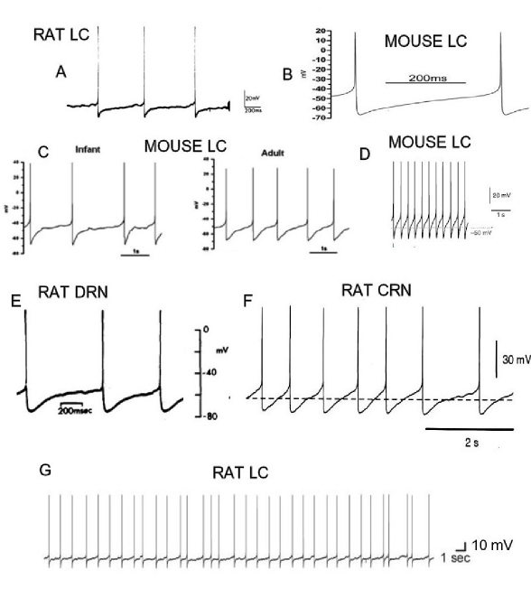
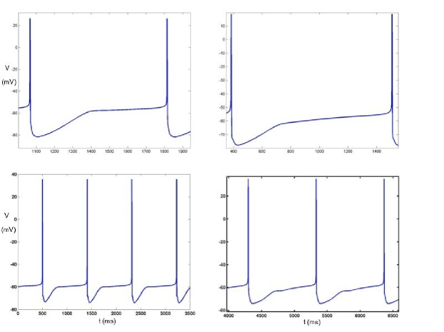
In Figure 1 are shown portions of spike trains in mouse and rat LC and rat DRN and CRN. It is noteworthy that the frequency of firing of LC and DRN principal neurons depend on sleep stage. Thus for example, in rats, waking , slow-wave sleep and REM sleep are accompanied by LC firing rates of about 2.2 Hz, 0.7 Hz and 0.02 Hz, respectively (Foote et al., 1980; Aston-Jones and Bloom, 1981; Luppi et al., 2012). Figure 2 shows computed spikes for the detailed model of rat DRN SE neurons of Tuckwell and Penington (2014) with 4 different parameter sets. In this model the main variables are membrane potential and intracellular calcium ion concentration which satisfy ordinary differential equations. There are, however, 11 membrane currents which drive the system which results in a system with 18 components and over 120 parameters. In order to study quantities like interspike interval distributions with various sources of random synaptic input, it is helpful to have a simpler system of differential equations which might yield insight into the properties of the complex model whose execution with random inputs over hundreds of trials would be overly time consuming. It is also pointed out that LC and DRN principal neurons are each responsive to activation of about 20 different receptor types, making computational tasks even more cumbersome with an 18-component model (Kubista and Boehm, 2006; Maejima et al., 2013). A simplified model of spike generation would be useful in modeling the dynamics of serotonin release and uptake (Flower and Wong-Lin, 2014).
2 Description of a two-component model
A first goal was to construct a two-component differential equation model whose solutions for the membrane potential broadly mimicked those for the muti-dimensional model developed in Tuckwell and Penington (2014), which gave satisfactory agreement with experimental voltage (see references in the preceding reference).
To this end the following pair of equations was found, with suitable choice of parameters, to have soutions with the desired properties. Here , in mV, is the depolarization of membrane potential from resting value and is a recovery variable. In keeping with the properties of the variables in the Fitzhugh-Nagumo equations (see for example Tuckwell, 1988, Section 8.8) will be (arbitrarily) ascribed units of mV/ms. Then we have
| (1) |
| (2) |
which system is usually to be solved with the initial conditions . The initial value of is usually set at the resting membrane potential so that whose average value for the cells of interest is -64.4 mV (Tuckwell, 2013).
For the application to spiking, it is assumed that the parameters , , , and are all positive. The zeros of the cubic
| (3) |
are chosen such that , with and .
3 Examples of results for the two-component model
In this section we give examples of computed solutions for the above two-component system and consider some of the properties of solutions.
Examples with two sets of parameters
There are ten parameters for the system of equations (1) and (2). Here we describe solutions for two sets of parameters, whose values are listed in Table 1. The solutions for both sets consist of periodic solutions in and where the first component mimics trains of action potentials.
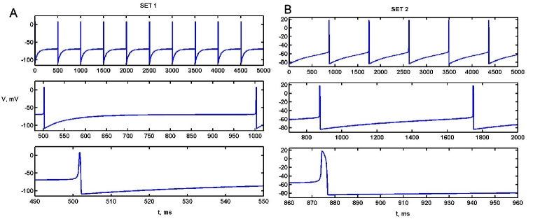
For parameter set 1 the (numerical) solutions are depicted in Figure 3 and some of the details of the solutions, such as maximum and minimum values of , mean ISI, mean duration measured at and maximum value of are given in the second column of Table 2. These results were obtained using an Euler scheme with ms.
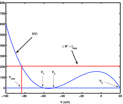
The voltage trajectories resemble in form some of the experimental ones in Figure 1, particularly for rat and mouse LC neurons (A and C), and to a lesser extent the rat DRN neurons (E). The duration of the action potential (measured at -40 mV) is only 0.55 ms, which is too short for these brainstem neurons. Furthermore, the AHP declines to a very low value of about -109 mV which is 49 mV below the assumed resting level. In order to make the minimum considerably higher in accordance with most experimental values, it is noted that the minimum of occurs when or when
| (4) |
where is the value of when the minimum of occurs. The graphical situation is shown in Figure 4. By judicious choice of values of the parameters, it was possible to obtain periodic solutions with minima of at an appropriate value of about -83 mV. This resulted in the parameter set 2 whose solution properties are displayed in column 3 of Table 2. These results were also obtained using an Euler scheme with step 0.02. The corresponding results with a step of ms are given in column 4. The latter much smaller value of should lead to more accurate solutions, but considering that the computing time was about 30 times longer and the change in solution properties such as ISI and duration were less than 1%, it is satisactory to use the larger time step. A comparison was also made with results obtained using a 4th order Runge-Kutta which was an order of magnitude slower than the Euler method and gave an almost identical ISI of 869.04 ms.
| Parameter | Set 1 | Set 2 | Parameter | Set 1 | Set 2 |
| 400 | 400 | -77.4 | -60 | ||
| 30 | 5 | -61 | -50 | ||
| 2 | 2 | 20 | 20 | ||
| -10 | -10 | 15 | 15 | ||
| 60 | 20 | 0.00042 | 0.0000525 |
| Property | Set 1 ( ms) | Set 2 ( ms) | Set 2 ms |
|---|---|---|---|
| Mean ISI (ms) | 501.1 | 870.8 | 869.5 |
| Mean Duration (ms) | 0.55 | 2.81 | 2.79 |
| Max (V) (mV) | +8.9 | +18.7 | +18.5 |
| Min(V) (mV) | -109.4 mV | -83.5 | -83.4 |
| Max(R) | 8.7 | 10.96 | 10.90 |
.
3.1 Frequency versus current curves
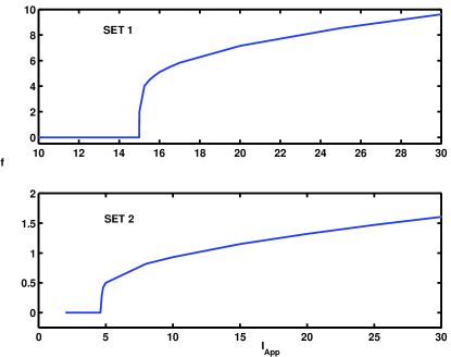
The above results for sets 1 and 2 parameters were all obtained with the . It is of interest to compute frequency of action potentials for various applied currents, as this corresponds to certain experimental data. The plot of output frequency versus applied current is called an f/I curve which differs in its characteristics from neuron to neuron. Often there is a threshold current for action potentials, which in the classical literature was called the rheobase current.
Hodgkin (1948) found for squid axon preparations that there were two broad types of f/I curves. Type 1 consisted of an f/I curve that smoothly rose from zero at a particular value of the input current, whereas type 2 curves discontinuously rose at a certain threshold current. Tateno et al. (2004) found that regular spiking and fast spiking neurons in the rat somatosensory cortex exhibit Type 1 and Type 2 firing behaviours, respectively. Mathematical explanations for the two types of threshold are found in the nature of the bifurcation which accompanies the transition from rest state to a periodic firing mode as discussed in Section 4.
Graphs of the frequency of repetitive spiking versus depolarizing input current are shown in Figure 5 for parameter sets 1 and 2. In both cases, at a particular value of the applied current the frequency jumps from zero to a positive value. For parameter set 1, the threshold current for firing is very close to 15 at which the firing frequency is about 2 Hz. For parameter set 2, the threshold curent is about at which the friring frequency jumps from zero to about 0.29 Hz. Thus the responses of the model with either parameter set are those of type 2 neurons (Hodgkin, 1948). The nature of the f/I curves for the approximate model is thus similar to that for both experimental results for DRN SE neurons and for the multi-component model (Tuckwell and Penington, 2014).
3.1.1 Autonomous pacemaker activity
The above results on frequency versus current have indicated that to make the model neuron fire with parameter sets 1 and 2, current must be applied. If this is necessary because the cubic defined in Eq. (3) is negative for a range of values of , and in particular the range containing . If , the cubic is tangential to the -axis, and is never negative. Then firing, albeit very slow, was demonstrated to occur for values of extremely close to zero, which would imply autonomous firing in the limit. It is possible by choosing a cubic with only one real root, for example at (as in parameter sets 1 and 2), so that for all , in which case autonomous firing could occur; that is with . The resulting source function would then be similar to the steady state curve in Figure 18 of the multidimensional model (Tuckwell and Penington, 2014) where in some cases it was found that pacemaker firing occurred in some cases for , or even whereas in others a small depolarizing drive was necessary.
4 Effects of changing parameters and phase plane analysis
A detailed compilation of the effects on the spike train properties as each of the ten parameters is varied is not explored here. Instead, Table 3 lists the effects of increasing or decreasing each of the ten parameter values relative to their values in set 2 on the mean ISI, mean duration of spike, maximum and minimum of voltage during spike, and maximum value of the recovery variable during spiking. We focus attention on the ISI and spike duration.
For the ISI, significantly altering each of the parameters , , and had little or no effect. On the other hand, the ISI was increased by decreasing any of , , and or by increasing either or . The duration of spikes was little affected by significant changes in any of , , , , or by decreases in , although increases in led to a substantial increase in duration. Significant increases in duration resulted from decreases in any of , or , or increases in .
| Parameters | Mean ISI | Mean Duration | Max(V) | Min(V) | Max(R) |
|---|---|---|---|---|---|
| Set 2 | 869.04 | 2.74 | 18.37 | -83.40 | 10.88 |
| 462.4 | 3.0822 | 0.26 | -91.92 | 4.53 | |
| 1231.84 | 4.0267 | 19.69 | -81.73 | 18.32 | |
| 849.32 | 5.47 | 19.84 | -82.15 | 9.87 | |
| 884.04 | 2.005 | 17.01 | -84.32 | 11.66 | |
| 853.02 | 4.58 | 19.58 | -82.40 | 20.14 | |
| 881.76 | 2.085 | 17.23 | -84.18 | 7.70 | |
| 1069 | 2.74 | 17.95 | -83.40 | 10.63 | |
| 755.52 | 2.74 | 18.78 | -83.40 | 11.13 | |
| 1127.82 | 2.8667 | 18.59 | -86.82 | 11.51 | |
| 794.7 | 2.66 | 18.10 | -80.15 | 10.27 | |
| 771.76 | 2.812 | 18.62 | -86.21 | 11.65 | |
| 1128.26 | 2.7067 | 18.05 | -80.78 | 10.14 | |
| 815.24 | 2.52 | 13.10 | -81.73 | 9.12 | |
| 919.14 | 3.025 | 23.63 | -84.99 | 12.80 | |
| 883.14 | 2.63 | 17.78 | -84.23 | 11.59 | |
| 840.84 | 3.14 | 18.86 | -81.82 | 9.62 | |
| 869.3 | 2.73 | 18.37 | -83.42 | 10.90 | |
| 868.76 | 2.75 | 18.36 | -83.38 | 10.87 | |
| 1396.54 | 2.74 | 18.37 | -83.42 | 10.89 | |
| 632.26 | 2.74 | 18.37 | -83.39 | 10.88 |
To see the bifurcations involved when the injected current is changed, we can analyze the phase plane of the model. The two nullclines of the two-component model are
| (5) |
for , and
| (6) |
for .
.
Depending on the parameters, the system may have one equilibrium or three equilibria. The voltage variable, , for each equilibrium, satisfies the equation
| (7) |
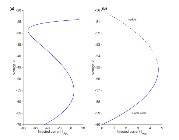
Solving equation (7) for the applied current , we find that the system goes through a saddle-node bifurcation when increases. In Figure (6a), the voltage in the equilibrium equation (7) is plotted with respect to the applied current . As we can see from Figure (6a), when , , and the other parameters are the same with parameter set 2, the system has three equilibria, visualized in Figure (7a) by the intersection of the cubic -nullcline and the -nullcline. In the lower voltage range, there is a stable node accompanied by a nearby saddle. The stable node corresponds to the resting state, and the saddle sets a threshold for the initial voltage required for there to be a (non-repetitive) spike. As the current increases, the distance between the stable node and the saddle decreases. Eventually the saddle and the node collide and annihilate each other through a saddle-node bifurcation, and the bifurcation diagram is as in Figure (6b). Once is larger than the bifurcation value, there is only one equilibrium which is an unstable focus, and the system has a limit cycle (see Figure 7b where ).

The system may also go through an Andronov-Hopf bifurcation when increases. For example, when , , , , , and all other parameters coincide with parameter set 2, then the system has only one equilibrium, which is a stable focus corresponding to the resting state (see Figure 7c). When is increased, the stable focus loses its stability, a limit cycle comes to exist (see Figure 7d), and the model exhibits spiking behavior.
From the theory of dynamical sytems (Ishikevich, 2007) spiking as a sequitur to either a saddle-node bifurcation or an Andronov-Hopf bifurcation results in a neuron with Type 2 dynamics as was found in the numerically generated f/I curves of Figure 6.
5 A reduced physiological model with two component currents
With the multi-component neuronal model for DRN SE neurons (Tuckwell and Penington, 2014) there are 11 component currents and a variety of solution behaviors for different choices of parameters. It is often difficult to see which parameters are responsible for various spiking properties. Some parameter sets lead to satisfactory spike trains with properties similar to experiment, but sometimes spike durations are unacceptably long. Other sets give rise to spontaneous activity but with spikes which have uncharacteristic large notches on the repolarization phase. Doublets and triplets are also often observed, and although these are sometimes found in experimental spike trains, it is desirable to find solutions depicting the regular singlet spiking and relatively smooth voltage trajectories usually observed.
In the previous section we have described a simplified two-component model whose first component representing membrane potential did resemble pacemaker spiking in certain brainstem neurons. An alternative model, with more parameters, can be constructed using full descriptions for the fast sodium transient currrent and the delayed rectifier potassium current as originally in the Hodgkin-Huxley (1952) model, but not including the leak current which may be approximately absorbed into an applied current . The emphasis is again on the membrane potential trajectories.
The basic differential equation for the voltage is
| (8) |
where C is capacitance, and is an added current in nA which depolarizes if negative. The initial value of is again taken to be resting potential, . All potentials are in mV, all times are in ms, all conductances are in S and capacitance is in nF.
Activation and inactivation variables are determined by the first order equations
| (9) |
| (10) |
where and are steady state values which depend on voltage. The quantities and are time constants which may also depend on voltage.
The fast transient sodium current, is given by the classical form
| (11) |
with activation variable and inactivation . For the steady state activation we put
| (12) |
with corresponding time constant
| (13) |
which fits well the forms used by some authors (McCormick and Huguenard, 1992; Traub et al., 2003) but not all. The steady state inactivation may be written
| (14) |
with corresponding time constant fitted with
| (15) |
We take the form for the delayed rectifier potassium current to be
| (16) |
where (the traditional symbol) is the activation variable which satisfies a differential equation like (6) and is the reversal potential. The steady state activation is written
| (17) |
and the time constant
| (18) |
5.1 Examples of pacemaker-like firing with two parameter sets
We illustrate the solutions with two choices of parameter sets. Set 1 is adopted from the parameters used for fast sodium and delayed rectifier potassium in the 11-current component model (Tuckwell and Penington, 2014) and the other is based in largely on values in Belluzi and Sacchi (1991) which we denote by Set 2. For the latter we also use the resting potential and the cell capacitance from Kirby et al. (2003), both being for rat DRN SE cells. The two sets of parameters are summarized in Table 4.
| Parameter | Set 1 | Set 2 |
|---|---|---|
| -33.1 | -36 | |
| 8 | 7.2 | |
| -50.3 | -53.2 | |
| 6.5 | 6.5 | |
| -60 | -67.8 | |
| 0.2 | 0.1 | |
| 1.0 | 2.0 | |
| C | 0.04 | 0.08861 |
| -15 | -6.1 | |
| 7.0 | 8.0 | |
| 1 | 1 | |
| - | 3.5 | |
| 1 | - | |
| 4 | - | |
| -20 | - | |
| 7 | - | |
| 2.00 | 1.5 | |
| 0.5 | 0.5 |
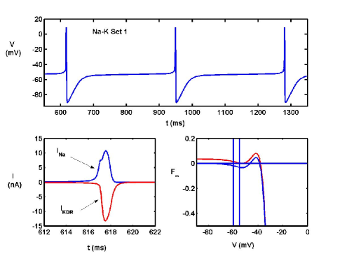
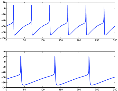
Both of these parameter sets led to repetitive spiking with the addition of a small depolarizing current. Typical spike trains are shown in Figures 9 and 10, and Table 5 contains lists of some of the details of the spike and spike train properties. Spiking for the second parameter set has a lower threshold for (repetitive) spiking, a longer ISI at threshold, a longer spike duration and a larger spike amplitude. For both parameter sets, most of these spike properties are in the ranges observed for DRN SE neurons. Figures 9 and 10 show well defined spikes with abruptly falling repolarization phases to a pronounced level of hyperpolarization followed by a steady increase in depolarization until an apparent spike threshold is reached.
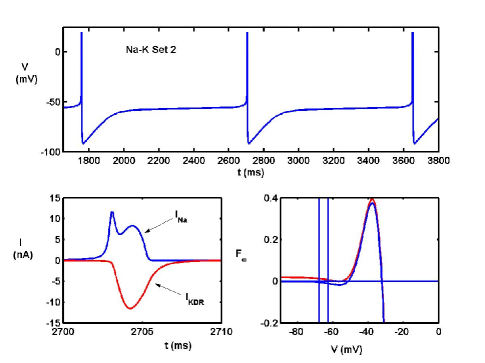
In the lower left-hand panels of Figures 9 and 10 are shown, on an expanded time scale, the fast sodium current and the delayed rectifier potassium current during spikes. In the lower right-hand panels are shown plots (thin blue curves) of the function defined as the sum of the steady state () values of the quantities of Equ. (8) and Equ. (13),
| (19) |
This behavior of this function near the resting potential has been found to provide a heuristic indicator for spiking (Tuckwell, 2013; Tuckwell and Penington, 2014). It can be seen in both Figures 9 and 10 that, for both parameter sets, the function is negative for in an interval of considerable size around the resting potential which is indicated by the vertical at -60 mV in Figure 9 and at - 67.8 mV in Figure 10. This means that around the derivative of with respect to time tends to be negative so that spontaneous spiking is unlikely. The magnitude of the smallest depolarizing current required to enable spiking is approximately the amount which must be added to make positive at and around . The resulting curves, shown in red in Figures 9 and 10, are approximately tangential to the V-axis, being obtained with for set 1 and for set 2 so that these values of are estimates of the threshold depolarizing current for (pacemaker) spiking.
DRN SE neurons often have characteristically long plateau-like phases in the latter part of the ISI and this is apparent in Figures 9 and 10 for spikes elicited near the threshold for spiking for both sets of parameters. The plateau for the second set is nearly three times as long as that for the first set. In both cases (not shown) at a particular value of the frequency jumps from zero to a positive value, being 3.0 Hz for set 1 and 1.1 Hz for set 2, so that this model with the chosen parameters would also be classified as one with Hodgkin type 2 neuron properties.
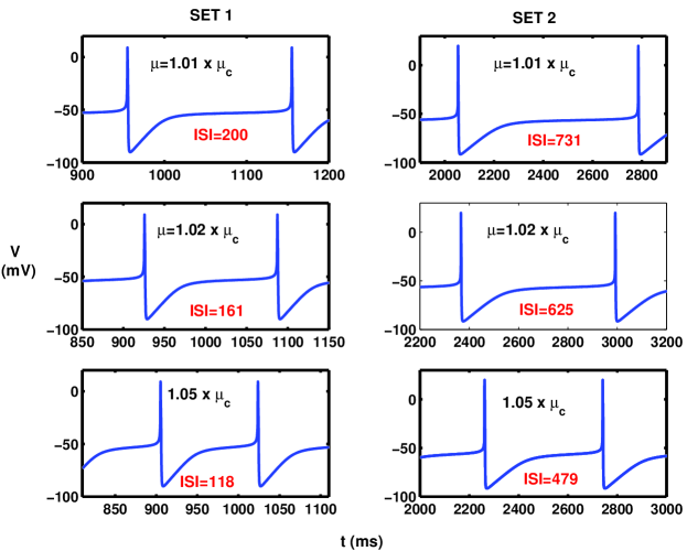
Figure 11 gives, for both parameter sets, the computed spike trajectories and ISIs for levels of excitation is not increased too much above threshold, being from 1 to 1.05 times the threshold values of . In each case the spike trajectory displays a typical pronounced and prolonged post-spike afterhyperpolarization followed by a plateau-like phase before the next spike.
Although the spiking properties for the two-current (Na-K) model have several features in common with both the experimental spike trains of DRN SE and LC NA neurons, with the parameter sets in Table 4, the frequency of action potentials is in accordance with experimental values near threshold, but as the level of excitation climbs to much greater values, the frequency becomes somewhat high (not shown) relative to the most commonly reported values for sustained firing in these brainstem neurons, although there are exceptions as the following examples illustrate. In rat LC neurons, Korf et al. (1974) found in unanesthetized vivo preparations, frequencies up to 30 Hz and Sugiyama et al. (2012) reported in vivo frequencies over 7 hz. In midbrain serotonergic raphe neurons, Kocsis et al. (2006) obtained in vivo rates with mean 5.4 Hz. For experiments with depolarizing current injection, Li and Bayliss (1998) obtained initial firing rates of around 8 Hz for caudal raphe with an injected current of 60 pA; Li et al. (2001) reported firing of rat DRN SE cells at frequencies as high as 35 Hz with current injection, and Ohliger-Frerking et al. (2003) found rates as high as 8 Hz and 11 Hz with 100 pA current injection in lean and obese Zucker rats, respectively.
| Property | Set 1 | Basic set 2 |
|---|---|---|
| Spike threshold | ||
| ISI at threshold | 331 ms | 948 ms |
| Spike duration (-40 mV) | 1.6 ms | 2.9 ms |
| Max V | +8 | +19.4 |
| Min V | -90.0 | -91.2 |
Hence the model is expected to be useful in predicting responses to random synaptic inputs in contradistinction to a sustained depolarizing current as employed in some experiments, which can lead to very large firing rates. However, with other parameter sets the model may not exhibit such high frequencies as depolarization level increases.
As Figure 1 shows, not all regular spiking in raphe and LC neurons entails a long afterhyperpolarization and a long plateau. Figure 11 shows that spikes similar to those in Figures 1B, 1D and 1F are generated in the second model with increased depolarizing current.
6 Discussion
The realistic mathematical modeling of brainstem neurons, beyond that provided by extremely simplified models such as the leaky integrate and fire (or Lapicque) model (Tuckwell, 1988), is needed in order to investigate the responses of these cells to their complex array of synaptic and other input and to construct and analyze complex networks involving these cells and those in other centers such as hippocampus, frontal cortex and hypothalamus.
6.1 LC NA neurons
Thus far there have been several mathematical models of locus coeruleus neurons per se, which include a few ionic channels (Putnam et al., 2014, abstract only) or many ionic channels including the usual sodium and potassium, high and low threshold calcium currents, transient potassium , persistent sodium, leak and hyperpolarization activated cation current (De Carvalho et al., 2000; Alvarez et al. 2002; Carter et al., 2012). Noteworthy is the omission of in the model of Alvarez et al. (2002) and its inclusion in De Carvalho et al. (2000) and Carter et al. (2012). Also, a persistent sodium current is included in De Carvalho et al. (2000) and Alvarez et al. (2002) but not in Carter et al. (2012).
Despite such uncertainties in the mechanisms involved in pacemaker activity in LC neurons, some of these works have included synaptic input and gap-junction inputs from neighboring LC neurons. The pioneering article of De Carvalho et al. (2000) addressed the mechanisms of morphine addiction and included several biochemical reactions involving cAMP, -opioid receptors, morphine, G-protein, AC, CREB and Fos. Tuckwell (2015) contains a summary of previous LC modeling as well as a review of LC neuron anatomy and physiology. Brown et al. (2004) did employ Rose-Hindmarsh model neurons to study a network of LC neurons but there have not appeared any plausible simplified models of these cells per se. Thus the two-component models considered in this article provide a good starting point for investigating, for example, the effects of synaptic input on LC firing which will be performed in future articles.
6.2 DRN SE neurons
For serotonergic neurons of the dorsal raphe there has been only one detailed model as described in the introduction (Tuckwell and Penington, 2014). Some authors have addressed quantitatively serotonin release and included the effects of antidepressants but without an explicit model for SE cell spiking (Geldof et al., 2008). Wong-Lin et al. (2012) use a quadratic integrate and fire model for spiking DRN SE neurons in a network of such cells along with inhibitory neurons. The model is not vastly different from the first model in this article, except that the reset mechanism after spikes is artificial. In a related work, Cano-Colino et al. (2013, 2014) have modeled the influence of serotonin on networks of excitatory and inhibitory cells in spatial working memory. More recently, in a similar vein, Maia and Cano-Colino (2015) have made an interesting study of serotonergic modulation of the strength of attractors in orbitofrontal cortex and related this to the occurrence of obsessive-compulsive disorder.
7 Concluding remarks
Principal brainstem neurons, particularly serotonergic cells of the dorsal raphe nucleus and noradrenergic cells of the locus coeruleus are of great importance in the functioning of many neuronal populations throughout cortical and subcortical structures. Of note is the modulatory role the firing of neurons in these brainstem nuclei have on neurons of the prefrontal cortex, including the orbitofrontal cortex, and hippocampus. These latter structures have been strongly implicated in various pathologies, including depression, and obsessive-compulsive disorders. Lanfumey et al. (2008) contains a comprehensive summary of many of the biological processes which are influenced by serotonin including those originating from serotonergic neurons of the DRN. Modeling networks involving both serotonergic and noradrenergic afferents requires plausible models for the spiking activity of the principal SE and NA cells. Whereas detailed models of such activity are now available, their application to many thousands of cells has the disadvantage of leading to very large computation time and large memory requirements, so that the simplified models described in the present article may provide useful approximating components for such complex computing tasks.
Acknowledgements
This research is supported by the National Science Foundation under Agreement No. 0931642 to YZ.
8 References
Alvarez, V.A., Chow, C.C., Van Bockstaele, E.J., Williams, J.T., 2002. Frequency-dependent synchrony in locus ceruleus: role of electrotonic coupling. PNAS 99, 4032-4036.
Amini, B., Clark, J.W. Jr, Canavier, C.C., 1999. Calcium dynamics underlying pacemaker-like and burst firing oscillations in midbrain dopaminergic neurons: A computational study. J. Neurophysiol. 82, 2249-2261.
Andrade. R., Aghajanian, G.K., 1984. Locus coeruleus activity in vitro: intrinsic regulation by a calcium-dependent potassium conductance but not -adrenoceptors J. Neurosci 4, .161-170.
Aston-Jones, G., Bloom, F.E., 1981. Activity of norepinephrine-containing locus coeruleus neurons in behaving rats anticipates fluctuations in the sleep-waking cycle. J. Neurosci. 1, 876-886.
Bayliss, D.A., Li, Y.-W., Talley, E.M., 1997a. Effects of serotonin on caudal raphe neurons: activation of an inwardly rectifying potassium conductance. J. Neurophysiol. 77, 1349–1361.
Belluzzi, O., Sacchi, O.,1991. A five-conductance model of the action potential in the rat sympathetic neurone. Prog. Biophys. Molec. Biol. 55: 1-30
Berridge, C.W., Waterhouse, B.D., 2003. The locus coeruleus–noradrenergic system: modulation of behavioral state and state-dependent cognitive processes. Brain Res. Rev. 42, 33-84.
Brown, E., Moehlis, J., Holmes, P. et al., 2004. The influence of spike rate and stimulus duration on noradrenergic neurons. J. Comp. Neurosci. 17, 13-29.
Cano-Colino, M., Almeida, R., Compte, A., 2013. Serotonergic modulation of spatial working memory: predictions from a computational network model. Frontiers in Integrative Neuroscience 7, 71.
Cano-Colino, M., Almeida, R., Gomez-Cabrero, D. et al., 2014. Serotonin regulates performance nonmonotonically in a spatial working memory network. Cerebral Cortex 24, 2449-2463.
Carter, M.E., Brill, J., Bonnavion, P. et al., 2012. Mechanism for hypocretin-mediated sleep-to-wake transitions. PNAS 109, E2635–E2644.
De Carvalho, L.A.V., De Azevedo, L.O., 2000. A model for the cellular mechanisms of morphine tolerance and dependence. Math. Comp. Mod. 32, 933-953.
De Oliveira, R.B., Howlett, M.C.H., Gravina, F.S. et al., 2010. Pacemaker currents in mouse locus coeruleus neurons. Neurosci 170, 166-177.
De Oliveira, R.B., Gravina, F.S., Lim, R. et al., 2011. Developmental changes in pacemaker currents in mouse locus coeruleus neurons. Brain Res. 1425, 27-36.
Flower, G., Wong-Lin, K., 2014. Reduced computational models of serotonin synthesis, release and reuptake. IEEE Trans. Biomed. Eng. 61, 1054-1061.
Foote, S.L., Aston-Jones, G., Bloom, F.E., 1980. Impulse activity of locus coeruleus neurons in awake rats and monkeys is a function of sensory stimulation and arousal. Proc. Nati. Acad. Sci. USA 77, 3033-3037.
Geldof, M., Freijer, J.I., Peletier, L.A. et al., 2008. Mechanistic model for the acute effect of fluvoxamine on 5-HT and 5-HIAA concentrations in rat frontal cortex. Eur. J. Pharm. Sci. 33, 217-219.
Hodgkin, A.L., 1948. The local changes associated with repetitive action in a non-medullated axon. J. Physiol. 107, 165-181.
Hodgkin, A.L., Huxley, A.F., 1952. A quantitative description of membrane current and its application to conduction and excitation in nerve. J. Physiol. 117, 500-544.
Jedema, H.P., Grace, A.A., 2004. Corticotropin-releasing hormone directly activates noradrenergic neurons of the locus ceruleus recorded in vitro. J. Neurosci. 24, 9703-9713.
Ishikevich, E. M., 2007. Dynamical systems in neuroscience: the geometry of excitability and bursting. MIT Press, Cambridge, Mass.
Ishimatsu, M., Williams, J.T., 1996. Synchronous activity in locus coeruleus results from dendritic interactions in pericoerulear regions. J. Neurosci. 16, 5196-5204.
Jacobs, B.L., Azmitia, E.C., 1992. Structure and function of the brain serotonin system. Physiol. Rev. 72, 165-229.
Kirby, L.G., Pernar, L., Valentino, R.J. et al., 2003. Distinguishing characteristics of serotonin and nonserotonin- containing cells in the dorsal raphe nucleus: electrophysiological and immunohistochemical studies. Neurosci. 116, 669-683.
Kocsis B, Varga V, Dahan L, Sik A (2006) Serotonergic neuron diversity: Identification of raphe neurons with discharges time-locked to the hippocampal theta rhythm. PNAS 103: 1059-1064.
Korf, J., Bunney, B.S., Aghajanian, G.K., 1974. Noradrenergic neurons: morphine inhibition of spontaneous activity. Eur.J. Pharmacol. 25, 165-169.
Kubista, H., Boehm, S., 2006. Molecular mechanisms underlying the modulation of exocytotic noradrenaline release via presynaptic receptors. Pharmacol. Therap. 112, 213-242.
Lanfumey ,L., Mongeau, R., Cohen-Salmon, C., Hamon, M., 2008. Corticosteroid-serotonin interactions in the neurobiological mechanisms of stress-related disorders. Neurosci. Biobehav. Rev. 32, 1174-1184.
Li, Y-Q., Li, H., Kaneko, T., Mizuno, N., 2001. Morphological features and electrophysiological properties of serotonergic and non-serotonergic projection neurons in the dorsal raphe nucleus An intracellular recording and labeling study in rat brain slices. Brain Res. 900, 110-118.
Li, Y-W., Bayliss, D.A., 1998. Electrophysiological properties, synaptic transmission and neuromodulation in serotonergic caudal raphe neurons. Clin. Exp. Pharm. Physiol. 25, 468-473.
Lowry, C.A., Evans, A.K., Gasser, P.J. et al., 2008. Topographic organization and chemoarchitecture of the dorsal raphe nucleus and the median raphe nucleus. In: Serotonin and sleep: molecular, functional and clinical aspects, p 25-68, Monti, J.M. et al., Eds. Basel: Birkhauser Verlag AG.
Luppi. P-H., Clement, O., Sapin, E. et al., 2012. Brainstem mechanisms of paradoxical (REM) sleep generation. Eur. J. Physiol. 463:43-52.
Maejima, T., Masseck, O.A., Mark, M.D., Herlitze, S., 2013. Modulation of firing and synaptic transmission of serotonergic neurons by intrinsic G protein-coupled receptors and ion channels. Frontiers in Integrative Neuroscience 7, 40.
Maia, T.V., Cano-Colino, M., 2015. The role of serotonin in orbitofrontal function and obsessive-compulsive disorder. Clinical Psychological Science 3, 460-482, and Supplemental-data.
McCormick, D.A., Huguenard, J.R., 1992. A model of the electrophysiological properties of thalamocortical relay neurons. J. Neurophysiol. 68, 1384-1400.
Ohliger-Frerking, P., Horwitz, B.A., Horowitz, J.M., 2003. Serotonergic dorsal raphe neurons from obese zucker rats are hyperexcitable. Neurosci. 120, 627-634.
Pan, W.J., Osmanović, S.S., Shefner, S.A., 1994. Adenosine decreases action potential duration by modulation of A-current in rat locus coeruleus neurons. J. Neurosci. 14, 1114-1122.
Penington, N.J., Kelly, J.S., Fox, A.P., 1991. A study of the mechanism of Ca2+ current inhibition produced by serotonin in rat dorsal raphe neurons. J. Neurosci. I7, 3594–3609.
Putnam, R., Quintero, M., Santin, J. et al., 2014. Computational modeling of the effects of temperature on chemosensitive locus coeruleus neurons from bullfrogs. Faseb J. 28, Supp. 1128.3. (Abstract only).
Ramirez, J-M., Koch, H., Garcia, A.J. III, et al., 2011. The role of spiking and bursting pacemakers in the neuronal control of breathing. J Biol. Phys. 37, 241-261.
Sanchez-Padilla,J., Guzman, J.N., Ilijic, E. et al., 2014. Mitochondrial oxidant stress in locus coeruleus is regulated by activity and nitric oxide synthase. Nat. Neurosci. 17, 832-842.
Sugiyama, D., Hur, S.W., Pickering, A:E. et al. 2012. In vivo patch-clamp recording from locus coeruleus neurones in the rat brainstem. J Physiol. 590, 2225-2231.
Swanson, L.W., 1976. The locus coeruleus: a cytoarchitectonic, golgi and immunohistochemical study in the albino rat. Brain Res. 110, 39-56.
Tateno,T., Harsch,A., Robinson,H.P.C., 2004. Threshold firing frequency- current relationships of neurons in rat somatosensory cortex: Type 1 and Type 2 dynamics. J. Neurophysiol. 92, 2283-2294.
Traub, R.D., Buhl, E.H., Gloveli, T., Whittington, M.A. 2003. Fast rhythmic bursting can be induced in layer 2/3 cortical neurons by enhancing persistent Na+ conductance or by blocking BK channels. J. Neurophysiol. 89, 909-921.
Tuckwell, H.C., 1988. Introduction to Theoretical Neurobiology. Cambridge University Press, Cambridge UK.
Tuckwell, H.C., 2013. Biophysical properties and computational modeling of calcium spikes in serotonergic neurons of the dorsal raphe nucleus. BioSystems 112, 204-213.
Tuckwell, H.C., 2015. Computational modeling of spike generation in locus coeruleus noradrenergic neurons. Preprint.
Tuckwell, H.C., Penington, N.J., 2014. Computational modeling of spike generation in serotonergic neurons of the dorsal raphe nucleus. Prog. Neurobiol. 118, 59-101.
Vandermaelen, C.P., Aghajanian, G.K., 1983. Electrophysiological and pharmacological characterization of serotonergic dorsal raphe neurons recorded extracellularly and intracellularly in rat brain slices. Brain Res. 289, 109–119.
Vasudeva, R.K., Waterhouse, B.D., 2014. Cellular profile of the dorsal raphe lateral wing sub-region: relationship to the lateral dorsal tegmental nucleus. J. Chem. Neuroanat. 57-58, 15-23.
Vertes, R.P., Crane, A.M., 1997. Distribution, quantification, and morphological characteristics of serotonin-immunoreactive cells of the supralemniscal nucleus (b9) and pontomesencephalic reticular formation in the rat. J. Comp. Neurol. 378, 411-424.
Williams, J.T., Egan, T.M., North, R.A., 1982. Enkephalin opens potassium channels on mammalian central neurons. Nature 299, 74-77.
Williams, J.T., Henderson, G., North, R.A:, 1985. Characterization of -adrenoceptors which increase potassium conductance in rat locus coeruleus neurones. Neuroscience 14, 95-101.
Wong-Lin, K-F., Joshi, A., Prasad, G., McGinnity, T.M., 2012. Network properties of a computational model of the dorsal raphe nucleus. Neural Netw. 32, 15-25.