The Influence of Spatial Resolution on Nonlinear Force-Free Modeling

Abstract

The nonlinear force-free field (NLFFF) model is often used to describe the solar coronal magnetic field, however a series of earlier studies revealed difficulties in the numerical solution of the model in application to photospheric boundary data. We investigate the sensitivity of the modeling to the spatial resolution of the boundary data, by applying multiple codes that numerically solve the NLFFF model to a sequence of vector magnetogram data at different resolutions, prepared from a single Hinode/SOT-SP scan of NOAA Active Region 10978 on 2007 December 13. We analyze the resulting energies and relative magnetic helicities, employ a Helmholtz decomposition to characterize divergence errors, and quantify changes made by the codes to the vector magnetogram boundary data in order to be compatible with the force-free model. This study shows that NLFFF modeling results depend quantitatively on the spatial resolution of the input boundary data, and that using more highly resolved boundary data yields more self-consistent results. The free energies of the resulting solutions generally trend higher with increasing resolution, while relative magnetic helicity values vary significantly between resolutions for all methods. All methods require changing the horizontal components, and for some methods also the vertical components, of the vector magnetogram boundary field in excess of nominal uncertainties in the data. The solutions produced by the various methods are significantly different at each resolution level. We continue to recommend verifying agreement between the modeled field lines and corresponding coronal loop images before any NLFFF model is used in a scientific setting.

1 Introduction

The solar coronal magnetic field produces solar activity, including extremely energetic solar flares and coronal mass ejections. There is considerable interest in accurate modeling of magnetic fields in and around active regions on the Sun, the locations of the most intense coronal fields and the drivers of flares and many mass ejections, with the aim of better understanding the physics underlying magnetic energy release, and improving the ability to predict space weather storms caused by large events.

A popular model for the coronal magnetic field $\boldsymbol{B}$ is the nonlinear force-free field (NLFFF) model (see the reviews by Wiegelmann & Sakurai 2012 and Régnier 2013), which assumes a static configuration with a zero Lorentz force,

$$\boldsymbol{J}\boldsymbol{\times}\boldsymbol{B}={\boldsymbol{0}},$$ (1)

where $\boldsymbol{J}=\mu_{0}^{-1}\boldsymbol{\nabla}\boldsymbol{\times}\boldsymbol{B}$ is the electric current density, together with the solenoidal condition,

$$\boldsymbol{\nabla}\boldsymbol{\cdot}\boldsymbol{B}=0.$$ (2)

The model current density is everywhere parallel to the magnetic field, and Equation (1) is often written

$$\boldsymbol{\nabla}\boldsymbol{\times}\boldsymbol{B}=\alpha\boldsymbol{B},$$ (3)

where $\alpha$ is the force-free parameter. The proper boundary conditions on the model are the specification of the normal component of the field $B_{n}$ over the bounding surfaces of the solution domain, together with the normal component of the electric current density $J_{n}$ (or, alternatively, $\alpha$) over one polarity of the field in the boundary (i.e., either over the region where $B_{n}>0$ or over the region where $B_{n}<0$) (Grad & Rubin 1958). The current density is only required over one polarity of the field because current density streamlines follow magnetic field lines, so values of $J_{n}$ at one polarity are “mapped” to the other polarity by the geometry of the field lines of the solution. Stated another way, taking the divergence of Equation (3) and applying the solenoidal condition yields the general property

$$\boldsymbol{B}\boldsymbol{\cdot}\boldsymbol{\nabla}\alpha=0,$$ (4)

which indicates that $\alpha$ is invariant along magnetic field lines (though $\alpha$ may be different from line to line). In the following, we consider the problem in a half space ($z>$ 0), with the plane $z$ = 0 representing the base of the (assumed force-free) corona. This geometry neglects solar curvature, which is appropriate for the local modeling done in this study.

Solar observations provide a set of boundary data for application of the model. Spectro-polarimetric measurements of magnetically sensitive lines (del Toro Iniesta 2003) are used to construct vector (three-component) magnetogram data that are presumed to be located on a planar surface representing the top of the photosphere. The vertical current density $J_{z}$ may be estimated from such vector magnetogram data using

$$\left.\mu_{0}J_{z}\right|_{z=0}=\left[\frac{\partial B_{y}}{\partial x}-\frac{\partial B_{x}}{\partial y}\right]_{z=0},$$ (5)

provided the 180-degree ambiguity in the direction of the field transverse to the line of sight is resolved (Metcalf et al. 2006; Leka et al. 2009).

Vector magnetogram data are now routinely produced by ground based instruments, and more recently have been provided by two space-based vector magnetographs: the Solar Optical Telescope/Spectro-Polarimeter (SOT-SP) on the Hinode satellite (Tsuneta et al. 2008), and the Helioseismic and Magnetic Imager on the Solar Dynamics Observatory (SDO/HMI; Schou et al. 2012). The use of such vector magnetogram data for NLFFF modeling builds on earlier work done with data from the Haleakala Stokes Polarimeter (HSP), the Imaging Vector Magnetograph (IVM), the Solar Flare Telescope (SFT), and the Advanced Stokes Polarimeter (ASP) in the previous decades (e.g., Mikic & McClymont 1994; Roumeliotis 1996; Thalmann & Wiegelmann 2008). The earliest vector magnetogram data possessed spatial resolutions of multiple arc seconds, whereas the Hinode/SOT-SP magnetogram data have a resolution as high as 0$\farcs$32.

In practice, however, additional modeling assumptions are needed in order to use vector magnetogram data with NLFFF modeling. One problem is that the boundary conditions on $J_{z}$ (or $\alpha$) are inconsistent with the NLFFF model over the two polarities of $B_{z}$ (Molodenskii 1969; Aly 1984, 1989). Additionally, boundary data are not available at the top and side surfaces of the three-dimensional solution domain. Furthermore, the vector magnetogram measurements contain uncertainties. The polarization measurements are subject to observational uncertainty, and the process of determining magnetic field values by inverting the Stokes polarization spectra involves making various assumptions about the radiative transport of polarized radiation through the magnetized solar atmosphere.

Given the scientific importance of determining the free energy in the solar coronal magnetic field, coupled with the recent increase in availability of vector data over the past decade, a sequence of yearly workshops was organized between 2004 and 2009 in an effort to characterize and improve NLFFF modeling. The workshops demonstrated that NLFFF methods work for analytic test cases and for synthetic, solar-like test data, but encounter specific problems in application to photospheric vector magnetogram data (Schrijver et al. 2006; Metcalf et al. 2008; Schrijver et al. 2008; De Rosa et al. 2009). There are a number of different methods of solution of the NLFFF model in use, which were found to produce significantly different results. Discrepancies include the locations and magnitudes of currents within the solution volume, and the total magnetic energy in the solution domain. Issues identified during these studies include the inconsistency of photospheric vector magnetogram data with the NLFFF model, the possibility that high spatial-resolution data are needed to account for small-scale currents, the limited field of view of the data, and the lack of account of the substantial uncertainties in the boundary field values.

More recently, additional NLFFF modeling workshops were held to address these issues. In this article, we follow up on one such issue and characterize the influence of the spatial resolution of vector magnetogram data on the results of the modeling. Examining this issue at this time is motivated by the increasing availability of vector data from various space- and ground-based instrumentation, all of which provide vector data at different spatial resolutions. For instance, the National Solar Observatory’s Synoptic Optical Long-term Investigations of the Sun Vector SpectroMagnetograph instrument (SOLIS/VSM) provides full disk data with a spatial sampling of 1$\farcs$1 (Henney et al. 2006, 2009), while SDO/HMI full-disk vector magnetograms have a pixel size of 0$\farcs$5 (Hoeksema et al. 2014), and “normal-map” and “fast-map” Hinode/SOT-SP data are sampled at 0$\farcs$16 and 0$\farcs$32 respectively (Lites et al. 2013).

To assess the sensitivity of the results of NLFFF modeling to variations in spatial resolution, we use data for NOAA Active Region (AR) 10978. Vector magnetograms are constructed from a Hinode/SOT-SP normal-map scan of this region, with the spatial resolution of the data artificially degraded by a sequence of binning factors. The methodology is to perform inversions on rebinned polarization spectra (as opposed to simply rebinning the resulting vector data inverted from spectra at the native Hinode/SOT-SP resolution) in order to approximate observations of AR 10978 by instruments having different spatial resolutions. In common with the earlier workshop studies, we apply a number of different methods of solution of the NLFFF model in order to also gauge the dependence of the results on the solution method.

The effects of spatial resolution on coronal field modeling have been discussed in several earlier studies. Parker (1996) claimed that the concentration of photospheric magnetic fields into unresolved fibrils renders currents inferred from vector magnetograms meaningless, but McClymont et al. (1997) argued in response that it is only necessary to resolve the large-scale twist in the field to correctly infer the current. Semel & Skumanich (1998) presented a method for inferring $|J_{z}|$ (for observations at disk center) that is independent of the ambiguity resolution, and argued for the reality of electric currents obtained using this method applied to ASP data. More recently, Leka et al. (2009) investigated the influence of noise and spatial resolution on the ambiguity resolution step in the treatment of vector magnetogram data (see also Georgoulis 2012, Leka et al. 2012, and Crouch 2013). A hare-and-hounds exercise was run on an analytic test case, and it was shown that failure to resolve observed structures due to low resolution leads to serious errors in ambiguity resolution.

Leka & Barnes (2012) also looked at the results of artificial degradation of Hinode/SOT-SP data on vector magnetic field values, including degrading observed Stokes spectra, and using full-resolution spectra but degrading the field values derived from the spectra. They examined, in particular, the effect of these steps on the statistics of the derived fields. They found that degraded resolution data can exhibit increased average flux densities, lower total flux, and field vectors shifted towards the line of sight. The distribution of $J_{z}$ was found to be very sensitive to the spatial resolution. Recently Thalmann et al. (2013) compared NLFFF reconstructions for an active region based on Hinode/SOT-SP and SDO/HMI data, including calculations for the Hinode data at original resolution and rebinned to match the HMI data. They found similar results for the different-resolution data from Hinode, but significantly different results for data between the two instruments, in particular, e.g., differences in magnetic connectivity. We note that Thalmann et al. (2013) rebinned vector magnetogram field values, rather than rebinning the original Hinode/SOT-SP spectral data as is done in the experiments presented here. Rebinning the spectra was shown in Leka & Barnes (2012) to produce different vector magnetogram values than rebinning the field values. These earlier studies motivate the present investigation of the influence of resolution on NLFFF modeling.

The structure of the paper is as follows. In Section 2 the data used and the different methods are presented, with Section 2.1 describing the preparation of the different resolution vector magnetograms, and Section 2.2 explaining the methods of solution of the NLFFF model, and their treatment of boundary conditions. In Section 3 we present a quantitative analysis of the energy and relative magnetic helicity of the resulting solution fields (Section 3.1), including assessment of non-solenoidal field errors, and an analysis of how the solution methods alter the vector magnetogram boundary data (Section 3.2). In Section 4, results are discussed and conclusions drawn.

2 Data and Methods

2.1 Vector Magnetogram Data for Active Region 10978

An ideal active region for this study would be one that is flux-balanced and is mostly isolated, shows evidence of nonpotentiality, is located near disk center, is small enough for the full active region to be observed with high-resolution spectropolarimetry, and has accompanying high-resolution coronal imagery suitable for comparisons between coronal loops and the field lines from the resulting extrapolations. Unfortunately, no such target satisfying all of these criteria was found from archive data. As a result, we prioritized the requirements for the nonpotentiality, location, isolation, and size for the magnetic field, and present in Section 3 performance metrics that do not rely on coronal loop data. Although some data from both the X-Ray Telescope (XRT) on Hinode and the Transition Region and Coronal Explorer (TRACE) instrument were available, there were an insufficient number of distinct and discernible loops for useful analysis.

Based on the above specifications, NOAA AR 10978 was selected from the archive of Hinode/SOT-SP observations. The SOT-SP instrument returns full Stokes spectra for the Fe I doublet at approximately 630.2 nm with high spectral sampling (2.15 pm). Polarization spectra for AR 10978 were obtained in normal-map mode on 2007 December 13, 12:18–13:41 UT

over a field of view of approximately 164$\arcsec\times$164$\arcsec$ (on a 1024$\times$1024 grid), with high spatial sampling (0$\farcs$16) both along the slit and in the direction of the scan.

Figure 1(a) shows a magnetogram of AR 10978 from the Michelson Doppler Interferometer (MDI; Scherrer et al. 1995) on board the Solar and Heliospheric Observatory (SOHO) on 2007 December 13. The region is isolated, being the only numbered active region on the disk at the time. The inset in Figure 1(b) shows the soft X-ray emission from the core of the region, as observed by Hinode/XRT. The core of the active region, where the strongest vertical currents (of critical importance to NLFFF modeling) are often located, lies within the Hinode/SOT-SP scan area, which is demarcated by the white boxes in Figures 1(a) and (b). Figures 1(c) and (d) illustrate the continuum intensity and the longitudinal magnetic field from Hinode/SOT-SP. The region is sufficiently small to allow the Hinode field of view to encompass most of the magnetic flux.

In the middle of its disk passage, AR 10978 possessed a Hale classification of $\beta\gamma$, indicating a high degree of flare productivity, and indeed almost 30 soft X-ray flares are attributed to the region in the National Geophysical Data Center GOES soft X-ray event lists over the course of its observed history on the solar disk. All were relatively small and short events. The largest flare was a very short and impulsive C4.5 flare which occurred at 09:39 UT on 2007 December 13, a few hours before the Hinode/SOT-SP normal-map scan used here was recorded. Additionally, the region produced a C1.0 flare within the hour following the completion of the scan.

Figure 1: Images of NOAA AR 10978 on 2007 December 13. Panel (a) shows the SOHO/MDI full-disk magnetogram at 12:46 UT, obtained within the interval of the Hinode normal-map scan used in this study. The image saturates at $\pm$1000 Mx cm${}^{\text{--2}}$. Panel (b) shows a logarithmically scaled Hinode/XRT images (Ti/Poly filter) averaged over the scan interval, for context. Representative Hinode/SOT-SP data are shown in the two smaller panels (both 162″$\times$162″) at right: panel (c) is the continuum intensity, and panel (d) shows the longitudinal magnetic field derived from the Hinode polarization spectra (scaled to $\pm$1500 Mx cm${}^{\text{--2}}$). The white boxes in panels (a) and (b) correspond to the region represented by panels (c) and (d). The black dashed outline in panel (d) indicates the region subsequently remapped into helioplanar coordinates for use in this study.

In this study, we construct a set of vector magnetograms from the chosen Hinode/SOT-SP scan of AR 10978 in order to investigate the effects of spatial resolution on the subsequent NLFFF extrapolations. Vector magnetograms are prepared at near-Hinode normal-map resolution, and also at spatial resolutions lowered by factors ranging from 2 to 16. The northernmost 25% of the Hinode field of view (mostly containing quiet sun) is excluded in order to make the subsequent NLFFF extrapolations more computationally tractable. The region considered for modeling is contained within the dashed box in Figure 1(d).

Because the codes used for NLFFF modeling in this paper assume a Cartesian geometry, it is necessary to project the Hinode data onto a regular helioplanar grid. The field of view of the Hinode observations is small relative to the solar radius, making the effects of curvature small, and as a result this remapping is not expected to significantly affect the modeling results. During the remapping process, $\boldsymbol{B}$ is reprojected so that it appears as if the active region were located at disk center. The resulting set of remapped vector magnetograms span a region approximately 168 Mm$\times$124 Mm in size. The local helioplanar coordinates are denoted $(x,y,z)$, with $x$ denoting solar west direction, $y$ solar north, and $z$ the vertical direction.

The procedure followed in preparing the vector magnetogram data at each resolution level is as follows: (1) the Level-1 Hinode/SOT-SP polarization spectra are rebinned by the specified factor; (2) a spectral inversion using the High Altitude Observatory Milne-Eddington inversion code (Skumanich & Lites 1987; Leka & Barnes 2012) is performed; (3) the 180^∘ disambiguity is resolved using the NorthWest Research Associates “ME0” minimum energy algorithm (Leka & Barnes 2012); (4) helioplanar components of $\boldsymbol{B}$, and values for the vertical component of the current density $J_{z}$ and force-free parameter $\alpha=\mu_{0}J_{z}/B_{z}$, are calculated; and (5) the resulting values are remapped (interpolated) onto a regular and uniformly spaced helioplanar grid.

Throughout this article, we refer to the various vector magnetograms by the factor by which the observed polarization spectra are rebinned in step (1). For example, “bin 2” data are rebinned by a factor of two in each dimension, “bin 3” data are rebinned by a factor of three in each dimension, etc. We also retain a “bin 1” dataset that is prepared without any rebinning. The grid and pixel sizes for these data as a function of the bin level are summarized in the first three columns of Table 1.

Table 1: Properties of AR 10978 Remapped Vector Magnetogram Data

Bin Level	Size (pixels)	Pixel Scale (Mm)	$\Phi/\Phi_{0}$	$F_{x}/F_{0}$	$F_{y}/F_{0}$	$F_{z}/F_{0}$	$F_{0}$ [N]
1	1129$\times$837	0.106	–0.030	08.3$\times$10${}^{\text{--4}}$	–1.1$\times$10${}^{\text{--2}}$	–0.37	2.4$\times$10${}^{\text{19}}$
2	0564$\times$418	0.212	–0.026	09.7$\times$10${}^{\text{--4}}$	–1.1$\times$10${}^{\text{--2}}$	–0.37	2.4$\times$10${}^{\text{19}}$
3	0375$\times$278	0.318	–0.024	–3.6$\times$10${}^{\text{--4}}$	–1.1$\times$10${}^{\text{--2}}$	–0.36	2.5$\times$10${}^{\text{19}}$
4	0282$\times$209	0.424	–0.026	–9.3$\times$10${}^{\text{--4}}$	–9.5$\times$10${}^{\text{--3}}$	–0.36	2.4$\times$10${}^{\text{19}}$
6	0187$\times$138	0.635	–0.024	–4.8$\times$10${}^{\text{--3}}$	–8.2$\times$10${}^{\text{--3}}$	–0.36	2.5$\times$10${}^{\text{19}}$
8	0141$\times$104	0.847	–0.026	–5.1$\times$10${}^{\text{--3}}$	–5.9$\times$10${}^{\text{--3}}$	–0.35	2.7$\times$10${}^{\text{19}}$
10	0112$\times$820	1.060	–0.031	–8.8$\times$10${}^{\text{--3}}$	–5.8$\times$10${}^{\text{--3}}$	–0.35	2.6$\times$10${}^{\text{19}}$
12	0093$\times$680	1.270	–0.029	–7.7$\times$10${}^{\text{--3}}$	–7.3$\times$10${}^{\text{--3}}$	–0.35	2.8$\times$10${}^{\text{19}}$
14	0080$\times$580	1.480	–0.030	–1.4$\times$10${}^{\text{--2}}$	–6.0$\times$10${}^{\text{--3}}$	–0.35	2.8$\times$10${}^{\text{19}}$
16	0070$\times$520	1.690	–0.038	–1.6$\times$10${}^{\text{--2}}$	–5.0$\times$10${}^{\text{--3}}$	–0.35	2.9$\times$10${}^{\text{19}}$

Uncertainties are provided for the components of $\boldsymbol{B}$, for $J_{z}$, and for the force-free parameter $\alpha$, based on propagation of uncertainties from the inversion and disambiguation steps. The disambiguation uncertainties comprise azimuthal errors of 180^∘ assigned to points where multiple trials of the disambiguation code produced different results with a frequency greater than 10% when the optimization procedure used is seeded with different sets of random numbers.

Figure 2 illustrates the reprojected vector magnetogram data. The figure shows maps of $B_{z}$ and $J_{z}$ for the bin 1 and bin 8 data (with the $J_{z}$ values shown only for points where the signal-to-noise ratio in $\alpha$ is greater than 0.25). We have set $\boldsymbol{B}={\boldsymbol{0}}$ at points in the reprojected coordinate system that lie outside of the Hinode field of view (such points are located at the eastern and western edges of the remapped data). The dashed boxes in the figure correspond to the region used for comparing NLFFF extrapolations in Section 3, and is slightly smaller than the remapped field of view. As expected, Figure 2 shows that large-scale structures present in $J_{z}$ at the photosphere are retained in the reduced-resolution data (albeit with a smaller magnitude), but structures on scales below the reduced resolution limit are lost.

Figure 2: The vertical magnetic field $B_{z}$, as derived from the Hinode data for AR 10978 and after remapping to helioplanar coordinates, at a resolution close to the Hinode observations (bin 1) is shown in panel (a), and the associated vertical current density $J_{z}$ is shown in panel (b). Panels (c) and (d) illustrate $B_{z}$ and $J_{z}$ after rebinning the Hinode data by a factor of eight and remapping into helioplanar coordinates. The color bars in each panel indicate the image scale in Mx cm${}^{\text{--2}}$ (for $B_{z}$) and mA m${}^{\text{--2}}$ (for $J_{z}$). The dashed boxes correspond to the base of the analysis volume used in Section 3 for comparing the resulting NLFFF solutions.

Figure 3: Images of continuum intensity for the (a) bin 1 and (b) bin 16 boundary data. The contours in panel (a) indicate the umbral (red) and penumbral (purple) boundaries derived from the bin 1 data, while those in panel (b) are derived from the bin 1 data and subsequently downsampled to the coarser resolution of the bin 16 data. In panel (b), it is evident that the downsampled umbral and penumbral contours do not exactly correspond to the analogous contours that would be drawn using the bin 16 continuum image.

Figure 4: Variations of the mean values of (a) unsigned vertical magnetic flux density $|B_{z}|$, (b) magnitude of the horizontal flux density $B_{h}=(B_{x}^{2}+B_{y}^{2})^{1/2}$, (c) magnitude of the vertical current density $|J_{z}|$, and (d) force-free parameter $\alpha$ that characterize the vector magnetogram data, as averaged over the full area and plotted as a function of spatial resolution. For clarity, we note that spatial resolution increases leftward (toward smaller pixel sizes) in each plot. In each panel, the averages over all pixels are shown in red, and averages over pixels inside the umbral and penumbral contours are shown in green and blue, respectively. Dashed curves indicate that the umbral and penumbral regions were determined from the rebinned data, and solid curves indicate that the regions were based on contours downsampled from the bin 1 data. (An example of contours that have been downsampled from bin 1 to bin 16 is shown in Fig. 3(b).) Error bars indicate standard deviations, except for panel (d) where standard errors are shown.

The structure of the magnetic field, which is inferred from the rebinned polarization spectra, is affected by the spatial resolution, sometimes in non-intuitive ways. Some of the trends depend on the underlying structure. To illustrate this effect, we use continuum intensity maps from Hinode/SOT-SP to segment the boundary data into umbral and penumbral regions. Figure 3(a) shows a bin 1 continuum intensity image with contours outlining umbral and penumbral regions overlaid. When downsampling the contours from the bin 1 data down to the resolution of the bin 16 data and comparing with the rebinned intensity image, as shown in Figure 3(b), differences between the downsampled contours and the locations of umbral and penumbral pixels are evident. This effect is especially noticeable in regions in the bin 1 data where small-scale features are present, leading to the classification of some pixels determined to be in the umbral region in the bin 1 image being identified as penumbral in the bin 16 image.

Figure 4 shows how the magnetogram-averaged absolute vertical flux density $|B_{z}|$, absolute horizontal flux density $B_{h}=(B_{x}^{2}+B_{y}^{2})^{1/2}$, $|J_{z}|$, and $\alpha$ vary as the spatial resolution changes. In the set of plots, the inferred values of these quantities are plotted as a function of spatial resolution in two ways, depending on whether the contours used in the segmentation are determined from the rebinned continuum images or are determined from downsampling those from the high-resolution bin 1 image. The differences between the two pairs of curves in $\left<|B_{z}|\right>$ and $\left<B_{h}\right>$ (Figs. 4(a) and (b)) as a function of resolution are often due to the spatial resolution affecting whether pixels are classified as being within the umbral or penumbral contours.

More strikingly, the average vertical current densities $\left<|J_{z}|\right>$ are seen to decrease as the spatial resolution decreases, indicating that the vertical currents often have structure on small scales. This effect also affects the trend in $\alpha$, with both umbral and penumbral values getting closer to zero (i.e., potential) as the spatial resolution decreases. The penumbral and umbral values of $\alpha$ possess different signs for most bin levels, though the mean $\alpha$ value in penumbral areas changes sign as the boundary data become less resolved.

Table 1 lists values of the net magnetic flux $\Phi$, and the components $F_{i}$ (with $i=x$, $y$, $z$) of the magnetic force on the coronal volume, as a function of the bin level. The flux is calculated by integrating $B_{z}$ over the magnetogram area, and the force components are obtained by performing the integrals in Molodenskii (1969), which are derived from moments of Equation (3). The net flux $\Phi$ is expressed as a fraction of the unsigned magnetic flux $\Phi_{0}$ (the integral of $|B_{z}|$ over the magnetogram area), and the force components are in units of $F_{0}$, the integral of the magnetic pressure over the magnetogram area. The net flux is zero if the observed area is in flux balance, and the force components vanish if the boundary data are consistent with the NLFFF model. The values in the table indicate that the region is close to flux-balanced. The region has relatively small horizontal force components and larger vertical forces (cf. Metcalf et al. 1995).

2.2 Methods and Codes Used

Many methods of solution of the NLFFF equations exist. In the study presented here, implementations of three such methods — the optimization, magnetofrictional, and Grad-Rubin methods — are applied to the sequence of vector magnetogram data described in Section 2.1. Altogether there are five codes (one code implementing the optimization method, one code implementing the magnetofrictional method, and three codes implementing the Grad-Rubin method in different ways).

Each of the five codes solves for a NLFFF on a uniform three-dimensional Cartesian grid with equal grid spacing in each dimension. The grids used are defined by the helioplanar vector magnetogram boundary data at the lower boundary and the choice of a vertical height for the grid. The codes differ in how they incorporate the vector magnetogram data at the lower boundary, and how they use the information provided by the uncertainties in the data. The boundary conditions at the side and top of the computational domain are not constrained by the observational data, and as a consequence the different codes handle boundary conditions at these surfaces in different ways. In the following subsections, we briefly describe each of the specific codes used in this study.

2.2.1 Optimization Method

The optimization method is a relaxation scheme that seeks to minimize a volume integral such that, if the integral becomes zero, the field is divergence- and force-free. In its original form (Wheatland et al. 2000), the method proceeds as follows. An initial magnetic field is chosen in the computational volume, and lower boundary values are replaced by the required vector boundary conditions $\boldsymbol{B}$. The field is evolved forward using equations that minimize a functional containing the magnitudes of the Lorentz force and of the divergence of $\boldsymbol{B}$. The process is halted when the field reaches an approximately steady state.

The optimization solutions discussed here are based on the algorithm described in Wiegelmann & Inhester (2010) and Wiegelmann et al. (2012), which includes several modifications to the original method. As discussed in Wiegelmann et al. (2006), the optimization solutions are found to improve when a preprocessing scheme is applied to the vector boundary data. Preprocessing reduces the magnitude of the integrals representing the boundary-integrated magnetic force and torque (which necessarily vanish for a NLFFF), subject to penalty functions that simultaneously aim to preserve agreement with the observed vector magnetogram data. Spatial smoothing is also applied to the boundary data. The specific preprocessing scheme used here involves four weighting parameters that determine which constraints are most closely met. The values used here are $\mu_{1}=\mu_{2}=1$ and $\mu_{3}=\mu_{4}=10^{\text{--3}}$, where the weighting parameters are as described in Equation (6) in Wiegelmann et al. (2006).

Additionally, modifications of the lower boundary values are permitted during the optimization process, implemented by including an additional optimization term in the functional that takes into account the measurement uncertainties in the vector magnetogram data. This term allows more substantial changes to the components of the field at points where the associated uncertainties are larger. These changes are controlled by a two-dimensional weighting matrix $\boldsymbol{W}(x,y)$ in an optimization integral over the lower boundary, as described in Wiegelmann & Inhester (2010).

The modified optimization method also includes three-dimensional weighting functions $w_{f}(x,y,z)$ and $w_{d}(x,y,z)$ in the functionals for the volume-integrated Lorentz force and divergence (see Equation (4) of Wiegelmann et al. 2012). These weights $w_{f}$ and $w_{d}$ are set to unity in the entire model volume, except for finite boundary layers adjacent to the lateral and top boundaries of the computational volume, where they smoothly approach zero. This causes the solution obtained by the method to remain fixed at the boundary values prescribed by the initial field, and introduces buffer regions at the side and top boundaries where the solution field may depart from a force-free and divergence-free state. These buffer regions are excluded from the analysis in Section 3.

Another feature of the optimization code used here is a grid-refinement scheme. The scheme entails applying the optimization code on coarser grids, the solutions of which are then used to initialize the optimization algorithm on successively more refined grids. Typically several refinement levels are used. The series of increasingly more refined grids is started by using a potential field to initialize the coarsest grid. This scheme has been shown in earlier studies to improve the quality of the resulting solutions to the NLFFF model, and decreases the running time of the full calculation.

2.2.2 Magnetofrictional Method

Magnetofrictional codes evolve the magnetic induction equation using a velocity field that advances the solution to a more force-free state (e.g., Chodura & Schlueter 1981). The magnetofrictional code used here is described in Valori et al. (2007, 2010), and its application to solar data is presented in Valori et al. (2012b). The magnetofrictional method uses the full vector field over the entire lower boundary as boundary condition, taking as input preprocessed vector magnetogram data. Both the horizontal and vertical components of $\boldsymbol{B}$ may be adjusted during the preprocessing stage to make the boundary data more compatible with the force-free model, although changes in the boundary data are constrained to be within certain limits (Fuhrmann et al. 2007, 2011).

As the field is evolved forward in time, the boundary conditions at the side and top boundaries are constructed by the code at each iteration of the magnetofrictional relaxation method using the neighboring volume values of the field at the previous iteration (Valori et al. 2007). The construction uses first order polynomial interpolation, and requires that the solenoidal condition is met at the boundary points, and that the Lorentz force falls to zero at ghost points just exterior to the volume.

A grid-refinement strategy analogous to that used in the optimization code is also used here. The domain having the coarsest refinement is initialized using a potential magnetic field with values of $B_{z}$ matching the initial preprocessed lower boundary values, and subsequent, more refined domains are initialized using the resulting fields from the less refined solutions.

For this particular active region, the magnetofrictional extrapolations of the full field of view at all tested resolutions developed abnormally strong but stable large-scale currents near the northern lateral boundary. Such behavior is unusual, and remained even after tuning the parameters of the algorithm. As a result, additional cropping of the magnetogram at the northern side was performed before running the magnetofrictional models shown here. In all but the case using bin 3 boundary data, the cropped magnetograms allowed the preprocessing algorithm to produce more compatible (more force-free) boundary conditions for the extrapolation code, and the resulting extrapolated fields did not develop any unusual current at the northern lateral boundary. For the bin 3 case, even this additional cropping did not yield a consistent preprocessed boundary condition, and consequently this case is omitted from the analyses presented in Section 3.

2.2.3 Grad-Rubin Method

Three different implementations of the Grad-Rubin method are used. These are the CFIT code (Wheatland 2007); the XTRAPOL code (as described in Amari et al. 2006 and with the boundary conditions given in Amari & Aly 2010); and the FEMQ code (Amari et al. 2006). A brief account of the specific implementations and boundary conditions is given here.

Grad-Rubin methods take as boundary conditions the normal component of the field in the boundary and the value of the force-free parameter $\alpha$ over one polarity of the field in the boundary. Since there are two choices of polarity there are two solutions, which are in general different if the boundary data are inconsistent with the force-free model. We present both solutions for all Grad-Rubin codes in this paper, using $P$ and $N$ to denote solutions with $\alpha$ chosen from positive- and negative-polarity regions in the lower boundary, respectively.

CFIT code

Grad-Rubin methods involve updates to both $\boldsymbol{B}$ and $\boldsymbol{J}$ at each iteration, involving the solution of linear hyperbolic and elliptic partial differential equations, respectively. The CFIT code performs the update to $\boldsymbol{J}$ by propagating lower boundary values of $\alpha$ along numerically traced field lines. The update to $\boldsymbol{B}$ is achieved by solving the Poisson equation for the vector potential for the field using a two-dimensional Fourier Transform method, with transforms in the $x$ and $y$ directions. Solutions from the code are correspondingly periodic in $x$ and $y$.

With the CFIT code, the lower boundary conditions on the field are the values of $B_{z}$ from the vector magnetogram data. Boundary conditions on $\alpha$ are chosen as follows. Values of $\alpha$ calculated using Equation (5) are used at a given boundary point provided the signal-to-noise ratio is at least 5%, based on the uncertainties provided with the data, and provided the boundary point does not exhibit a large localized spike in $\alpha$. Boundary points not meeting these criteria are assigned values $\alpha=0$. This procedure is referred to as “censoring” of the boundary data.

Additionally, during the Grad-Rubin iteration procedure, points in the domain that are threaded by field lines that intersect the top or side boundaries are assigned $\alpha=0$ to ensure $\boldsymbol{\nabla}\boldsymbol{\cdot}\boldsymbol{J}=0$ globally. As a result, boundary points in such open-field regions are treated as having $\alpha=0$, however the regions of open and closed field lines generally change as the calculation proceeds, and consequently boundary points that are thus censored at one iteration may not be censored at another.

The iteration is initiated with a potential field in the volume with values of $B_{z}$ matching the vector magnetogram at the lower boundary values, obtained by a two-dimensional Fourier transform solution. The CFIT code is parallelized using both the OpenMP (Chandra et al. 2001) and MPI (Gropp et al. 1999) standards. Further details on the solution method and the handling of boundary conditions are given in Wheatland (2007).

XTRAPOL code

The XTRAPOL code solves a mixed elliptic-hyperbolic boundary-value problem for $\alpha$ and $\boldsymbol{B}$, which is mathematically well posed (Boulmezaoud & Amari 2000). It uses a finite-difference approach with a representation of $\boldsymbol{B}$ based on a vector potential $\boldsymbol{A}$ (defined with a convenient gauge) on a staggered mesh. This ensures that the divergence operator remains exactly on the kernel of the curl operator (and thus $\boldsymbol{\nabla}\boldsymbol{\cdot}\boldsymbol{B}=0$ to rounding errors), independently of the mesh resolution. It solves iteratively the elliptic problem through a positive definite linear system, and the hyperbolic problem by transporting $\alpha$ along the characteristics (the magnetic field lines), imposing $\alpha$ originating from only one or the other polarity. The code uses the MPI library. The solution can be provided for both balanced or non-balanced photospheric magnetic flux, in which case field lines can intersect other external boundaries. See Amari et al. (2006) for more details.

FEMQ code

The FEMQ code solves the same well posed boundary-value problem as XTRAPOL. However FEMQ uses a finite-element approach, and works directly with $\boldsymbol{B}$ using a least-squares approach that minimizes the divergence of $\boldsymbol{B}$. The hyperbolic equations at each iteration can be solved either using the same method as in XTRAPOL or by solving a non-positive-definite linear system for $\alpha$ by an iterative method. More details can be found in Amari et al. (2006).

3 Results

This section presents quantitative comparisons amongst the extrapolated solution fields and characterizes the effects of the spatial resolution of the boundary data on the solutions. We analyze the energy and helicity of the solutions and discuss the departure of the lower boundary field values in the resultant solutions from the vector magnetogram values. The magnetic energy analysis includes a Helmholtz decomposition of the solution fields into solenoidal and non-solenoidal components, following the procedure of Valori et al. (2013), and a discussion of the effects of the non-solenoidal component on the resulting energies. Because physical magnetic fields are solenoidal (due to $\boldsymbol{\nabla}\boldsymbol{\cdot}\boldsymbol{B}=0$), comparing the non-solenoidal and solenoidal components provides a check on the consistency of the solutions.

Performing a NLFFF extrapolation using the bin 1 data remains a challenge for the codes and for computer hardware. An extrapolated field $\boldsymbol{B}$ corresponding to these data and represented by a single-precision, floating-point, three-dimensional array possesses of order $N^{\text{3}}\approx$1000${}^{\text{3}}$ points and requires $\approx$12 GB of computer memory. The codes as written require multiple copies of this and similar three-dimensional arrays to be stored simultaneously in computer memory. As a result, memory use is an issue. A more constraining factor is the scaling of the time to completion, taken to be at best $\propto N^{\text{4}}$ for serial calculation on a grid with $N^{\text{3}}$ points (e.g., Wheatland 2007). A number of the methods employ parallel implementations to improve performance, but the total computational time remains a problem for large grids. As a result of these constraints, we do not present the results obtained for the bin 1 data.

Results are presented for bin levels 2–16 for all five codes (the optimization and magnetofrictional method codes, and the CFIT, XTRAPOL and FEMQ Grad-Rubin codes), with the exception of the magnetofrictional solution using the bin 3 boundary data. For the three Grad-Rubin codes, results are presented for both the $P$ and $N$ cases. Altogether, there are 71 solution data cubes.

For a given resolution level, the five codes employ domains that are slightly different. To standardize the comparisons across codes and resolutions, we will use a fixed analysis volume $\mathcal{V}$, chosen to be the largest common physical volume for all solutions across codes and resolutions. This analysis volume is 136$\times$77$\times$107 Mm${}^{\text{3}}$ and covers approximately the region from $x$ = 14.3 Mm to $x$ = 150.0 Mm, from $y$ = 14.3 Mm to $y$ = 92.8 Mm, and from $z$ = 0 Mm to $z$ =107 Mm, where the origin is located at the lower left-hand corner of the input magnetograms. The footprint of the analysis volume $\mathcal{V}$ on the photosphere is indicated by the dashed lines in the vector magnetogram data shown in Figure 2.

Figure 5 presents visualizations of field lines within $\mathcal{V}$ for the solutions for the different methods for the finest resolution level for which there are solution data. Qualitatively, it is evident that there are some differences between the results obtained with the different methods or codes at this resolution. Such variation across the solution methods is in common with our earlier studies (e.g., Schrijver et al. 2006; Metcalf et al. 2008; Schrijver et al. 2008; De Rosa et al. 2009). When examining the differences in solution data across the range of resolution levels, as calculated by any of the codes, the initial qualitative impression is that there are only minor differences in (for example) the detailed field-line trajectories. The shape of the field-line bundles originating in different locations across the lower boundary of the analysis region appears similar for all resolutions, and the boundaries separating field lines that leave the analysis volume versus those that are contained within the domain appear similar. In the sections that follow, we show that more significant variations exist amongst the solutions, both across resolution levels and across methods and codes, when quantitative comparisons are performed.

Figure 5: Field lines for all solutions using the bin 2 boundary data. The panels show results using the (a) CFIT Grad-Rubin ($P$ solution), (b) CFIT Grad-Rubin ($N$ solution), (c) optimization, (d) XTRAPOL Grad-Rubin ($P$ solution), (e) XTRAPOL Grad-Rubin ($N$ solution), (f) magnetofrictional, (g) FEMQ Grad-Rubin ($P$ solution), and (h) FEMQ Grad-Rubin ($N$ solution) codes. For comparison, field lines from a potential field matching the values of $B_{z}$ provided to the modelers are shown in panel (i). Field lines are plotted in black, green, and magenta: black field lines close within the volume, whilst the magenta and green field lines are open, and originate in different polarities. The starting points for the field line trajectories form a regularly-spaced grid at $z=0$.

Figure 6: (a) Total magnetic energy $E$, (b) energy of the associated potential field $E_{\text{0}}$, (c) free energy $E_{f}=E-E_{0}$, and (d) ratio $E/E_{\text{0}}$, as a function of spatial resolution for the set of NLFFF calculations. Please note that resolution increases to the left in each plot (i.e., smaller pixel sizes and smaller bin factors correspond to more highly resolved boundary data).

3.1 Magnetic field energy, helicity and extrapolation metrics

In this section, the magnetic energies $E$, the relative magnetic helicities $H_{m}$ of the extrapolated magnetic fields, and additional extrapolation metrics are discussed. The variations amongst the energies and helicities of the extrapolated fields depend on many factors, including the effects of resolution, the boundary conditions taken as input, and the handling of boundary conditions by the various codes. An additional consideration is that, for each resolution level, the same numerical grid is used for the calculation of these quantities, regardless of code and method, with interpolation onto this grid performed when necessary (such as when analyzing results from XTRAPOL, in which variables are offset with each other on a staggered mesh). Centered, second-order finite differences are used to calculate the needed derivatives, and this differencing scheme may also be different than the one used by the various codes (e.g., the magnetofrictional code uses fourth-order differences).

3.1.1 Magnetic Energy

Figure 6 illustrates the magnetic energy $E$, the magnetic energy of the corresponding reference potential field $E_{0}$, the free energy $E_{f}=E-E_{0}$, and the ratio $E/E_{0}=1+E_{f}/E_{0}$ as a function of spatial resolution for each of the extrapolations within the common analysis volume $\mathcal{V}$. The reference potential fields are computed numerically by solving the Laplace equation for the potential with Neumann boundary conditions based on the normal component of $\boldsymbol{B}$ on all six boundaries of the analysis volume (which we denote $B_{n}|_{\partial\mathcal{V}}$). Following Thomson’s theorem (e.g., Jackson 1999), the potential field uniquely represents the field with the minimum energy for any divergence-free field where $B_{n}$ matches $B_{n}|_{\partial\mathcal{V}}$. As a consequence of each solution field having its own $B_{n}|_{\partial\mathcal{V}}$, there are separate reference potential fields for each of the solution fields.

Table 2: NLFFF Extrapolation Metrics for AR 10978

Method/Code	Bin	$E$ [10${}^{\text{26}}$ J]	$E/E_{\text{0}}$	$H_{m}$ [10${}^{\text{26}}$ Wb${}^{\text{2}}$]	$\left<\text{CW}\sin\theta\right>$	$\left<|f_{i}|\right>$ [$\times$10${}^{\text{--4}}$]	$\xi$
Optimization	16	1.41	1.12	string0.66	0.13	19.00	0.38
	14	1.38	1.14	string0.03	0.14	18.00	0.37
	12	1.43	1.18	–0.16	0.12	16.00	0.39
	10	1.39	1.15	–0.24	0.14	10.00	0.33
	8	1.46	1.18	string0.47	0.11	06.10	0.23
	6	1.43	1.18	–0.63	0.11	03.70	0.21
	4	1.48	1.21	string0.24	0.10	02.20	0.18
	3	1.47	1.20	–0.92	0.13	01.70	0.19
	2	1.50	1.24	string0.04	0.10	01.10	0.16
Magnetofrictional	16	1.37	1.16	1.29	0.30	82.00	0.51
	14	1.22	1.15	3.79	0.30	71.00	0.51
	12	1.23	1.17	2.62	0.32	52.00	0.53
	10	1.26	1.19	3.65	0.25	46.00	0.51
	8	1.28	1.14	4.89	0.31	33.00	0.34
	6	1.11	1.09	3.17	0.29	18.00	0.51
	4	1.23	1.12	3.96	0.27	13.00	0.26
	2	1.08	1.10	1.80	0.29	13.00	0.34
CFIT ($P$ / $N$)	16	1.12 / 1.12	1.04 / 1.03	3.55 / 3.43	0.35 / 0.40	11.0/ 12.0	0.08 / 0.09
	14	1.09 / 1.08	1.06 / 1.04	4.14 / 3.38	0.32 / 0.38	09.9 / 11.0	0.07 / 0.10
	12	1.11 / 1.11	1.05 / 1.04	3.56 / 3.95	0.32 / 0.36	07.6 / 09.8	0.06 / 0.10
	10	1.09 / 1.09	1.05 / 1.05	3.51 / 4.23	0.32 / 0.34	06.5 / 08.6	0.08 / 0.11
	8	1.12 / 1.12	1.05 / 1.05	3.32 / 4.58	0.32 / 0.31	06.4 / 07.3	0.12 / 0.13
	6	1.11 / 1.09	1.07 / 1.05	4.05 / 3.68	0.27 / 0.29	04.7 / 06.1	0.10 / 0.14
	4	1.19 / 1.16	1.11 / 1.10	5.21 / 3.88	0.28 / 0.30	05.0 / 06.1	0.21 / 0.24
	3	1.11 / 1.11	1.06 / 1.06	2.45 / 2.95	0.27 / 0.26	04.0 / 04.8	0.21 / 0.24
	2	1.12 / 1.10	1.06 / 1.05	4.47 / 2.32	0.24 / 0.25	02.1 / 03.4	0.19 / 0.25
XTRAPOL ($P$ / $N$)	16	1.29 / 1.29	1.02 / 1.02	2.68 / 2.30	0.26 / 0.25	7.90/ 7.80	0.03 / 0.03
	14	1.25 / 1.25	1.03 / 1.03	3.01 / 3.01	0.25 / 0.24	6.70/ 6.50	0.03 / 0.02
	12	1.28 / 1.27	1.03 / 1.03	3.21 / 2.99	0.24 / 0.22	6.00/ 5.70	0.03 / 0.02
	10	1.27 / 1.26	1.04 / 1.03	3.99 / 2.75	0.21 / 0.19	5.10/ 4.70	0.03 / 0.02
	8	1.29 / 1.28	1.04 / 1.04	3.47 / 3.24	0.21 / 0.18	3.10/ 3.00	0.02 / 0.02
	6	1.27 / 1.26	1.05 / 1.04	3.45 / 2.72	0.17 / 0.16	2.20/ 2.10	0.02 / 0.02
	4	1.29 / 1.28	1.05 / 1.05	3.52 / 4.13	0.13 / 0.16	1.20/ 1.20	0.02 / 0.04
	3	1.28 / 1.27	1.05 / 1.04	3.40 / 2.83	0.12 / 0.12	0.83 / 0.77	0.02 / 0.02
	2	1.28 / 1.28	1.05 / 1.05	3.46 / 2.24	0.14 / 0.13	0.46 / 0.40	0.08 / 0.06
FEMQ ($P$ / $N$)	16	1.29 / 1.30	1.04 / 1.03	2.87 / 2.50	0.28 / 0.25	6.40/ 6.90	0.02 / 0.02
	14	1.25 / 1.25	1.03 / 1.03	3.32 / 3.14	0.26 / 0.26	5.20/ 5.30	0.02 / 0.02
	12	1.28 / 1.28	1.03 / 1.03	3.24 / 3.06	0.25 / 0.24	4.50/ 4.60	0.02 / 0.02
	10	1.27 / 1.26	1.04 / 1.04	3.87 / 2.70	0.22 / 0.20	3.50/ 3.50	0.02 / 0.02
	8	1.29 / 1.28	1.05 / 1.04	3.93 / 3.50	0.21 / 0.19	2.80/ 2.80	0.02 / 0.02
	6	1.27 / 1.26	1.05 / 1.04	3.65 / 2.65	0.17 / 0.15	1.80/ 1.70	0.02 / 0.01
	4	1.30 / 1.28	1.05 / 1.05	3.66 / 3.87	0.12 / 0.15	0.99 / 0.98	0.01 / 0.04
	3	1.29 / 1.28	1.05 / 1.04	3.34 / 2.79	0.11 / 0.11	0.69 / 0.66	0.04 / 0.03
	2	1.29 / 1.28	1.06 / 1.05	3.87 / 2.97	0.10 / 0.11	0.42 / 0.38	0.07 / 0.07

Figure 7: The decomposition of the total energy into solenoidal ($\widetilde{E}_{\text{0,s}}$ and $\widetilde{E}_{\text{J,s}}$) and non-solenoidal ($\widetilde{E}_{\text{0,ns}}$, $\widetilde{E}_{\text{J,ns}}$, and $|\widetilde{E}_{\text{mix}}|$) contributions, for the different solutions. The individual panels show results for the (a) magnetofrictional, (b) optimization, (c) CFIT, (d) XTRAPOL, and (e) FEMQ codes. The different contributions are shown as a function of resolution. The tilde over each term indicates normalization to the corresponding total energy $E$. Table 4 in Appendix A lists the numerical values of all contributions for each solution.

The energy metrics are listed in Table 2. Taken as a group, the energies of the solution fields range from 1.08$\times$10${}^{\text{26}}$ J to 1.50$\times$10${}^{\text{26}}$ J, with a mean value of 1.25$\times$10${}^{\text{26}}$ J and a standard deviation of 10%. In terms of free energy $E_{f}$, the solutions range from near-potential fields having free energy 2% above $E_{0}$ (both $P$ and $N$ models of XTRAPOL using the bin 16 boundary data) to a case where the free energy is 24% of the associated potential field (optimization using the bin 2 boundary data). In physical units, the free energy $E_{f}$ is in the range 0.3–2.9$\times$10${}^{\text{25}}$ J.

Figures 6(c) and (d) show that the solutions obtained with the magnetofrictional and optimization methods have higher free energies than those calculated using Grad-Rubin methods (CFIT, XTRAPOL, and FEMQ), both in absolute ($E-E_{0}$) as well as in relative ($E/E_{0}$) terms. When more highly resolved boundary data are used, all methods return solutions that trend toward higher energies, with the exception of the magnetofrictional method. Figure 6 illustrates that the free energies for the magnetofrictional method range from 10% to 19%, with higher resolution cases generally having less free energy. In contrast, the free energies from the optimization method increase as the resolution increases from 12% to 24%. The free energies in the Grad-Rubin codes are also seen to double over the range of resolutions, becoming greater for the more spatially resolved cases (as with the optimization method), though this variation corresponds to changes of a few percent of the total magnetic energy. Within the set of Grad-Rubin solutions, the relative free energy values are slightly higher at all resolutions for CFIT than for FEMQ and XTRAPOL. Free energies for the $P$ solutions are equal or marginally higher than those from the $N$ solutions. At each resolution value, the spread in free energies for the Grad-Rubin codes appears small, with the exception of the CFIT calculations using the bin 4 boundary data (addressed further in the next subsection).

Two aspects of the calculation methods may explain the spreads in total and free energies. First, the larger spread in energies from the optimization and magnetofrictional solutions may be attributed in part to their divergences, as evaluated numerically, being greater than the Grad-Rubin methods (which is expected on the basis of past results, see, e.g., Schrijver et al. 2006, 2008; De Rosa et al. 2009). These methods introduce a departure from $\boldsymbol{\nabla}\boldsymbol{\cdot}\boldsymbol{B}=0$ upon initialization, and then seek to minimize this error during iteration. In contrast, the Grad-Rubin implementations employ schemes that are initialized with divergence-free fields, and aim to provide divergence-free fields at all iterations. (We further address the contribution from residual non-solenoidal field components to the total energy in the next subsection.)

Second, the higher energies of the magnetofrictional and optimization solutions may be due in part to the preprocessing used with these methods. As was the case in Metcalf et al. (2008) and Schrijver et al. (2008), preprocessing the boundary data to be more compatible with the force-free assumption can result in solution fields having greater free energies. All Grad-Rubin implementations presented here remove spikes in $\alpha$ (many of which likely result from poorly constrained values of $B_{x}$ and $B_{y}$), but do not otherwise preprocess the boundary data. The degree to which the codes necessarily alter the boundary data are discussed further in Section 3.2.

3.1.2 Energy Decomposition

Accurate numerical solutions to the force-free model should be solenoidal, to within numerical errors. However, the methods of solution to the equations, and the inconsistency of the boundary data with the model, can lead to significant departures from solenoidality. Valori et al. (2013) provide a method for quantifying how much a non-zero divergence in a NLFFF solution affects the accuracy of the estimate for the magnetic field energy. The Valori et al. (2013) method is an application of Thomson’s theorem. The magnetic field is decomposed into a potential and a current carrying part, and each of these is split into solenoidal and non-solenoidal components via Helmholtz decomposition. The energies of the components are then compared. In this section, we summarize the decomposition as applied to each of the NLFFF calculations, leaving the details to Appendix A.

The magnetic energy within $\mathcal{V}$ may be written

$$E = \frac{1}{2\mu_{0}}\int_{\mathcal{V}}{B^{2}}\,{\text{d}}\mathcal{V}$$ (6)

$$= E_{\text{0,s}}+E_{\text{J,s}}+E_{\text{0,ns}}+E_{\text{J,ns}}+E_{\text{mix}}\,,$$

where $E_{\text{0,s}}$ and $E_{\text{J,s}}$ are the energies of the potential and current-carrying solenoidal components, $E_{\text{0,ns}}$ and $E_{\text{J,ns}}$ are those of the non-solenoidal components, and $E_{\text{mix}}$ is a non-solenoidal mixed term (see Equations (7) and (8) in Valori et al. 2013 for the expressions for the energies in terms of the field components). The energies in Equation (6) are positive by definition, with the exception of $E_{\text{mix}}$. For a perfectly divergence-free field, $E_{\text{0,s}}=E_{\text{0}}$ and $E_{\text{J,s}}=E_{f}=E-E_{\text{0}}$, while $E_{\text{0,ns}}=E_{\text{J,ns}}=E_{\text{mix}}=0$. In practice, a NLFFF calculated numerically will not be perfectly solenoidal, and $E_{\text{0,ns}}$, $E_{\text{J,ns}}$, and $E_{\text{mix}}$ will instead be finite. Comparing the non-solenoidal components with the free energy can be used to gauge the reliability and uncertainty of the free energy determination.

The values of each term in Equation (6) for each method and spatial resolution are plotted in Figure 7. For the Grad-Rubin methods, the results are plotted for both the $N$ and $P$ solutions using identical (and often overlapping) symbolism. Figure 7 shows that the energies contained in the non-solenoidal components are generally lower than the solenoidal portions. The primary exceptions to this trend are with the optimization solutions, where the magnitudes of the mixed terms $|E_{\text{mix}}|$ for all resolution levels are of the same order as the free energy $E_{\text{J,s}}$. The energy of the non-solenoidal component of the potential field $E_{\text{0,ns}}$ is smaller by at least a factor of 10${}^{\text{3}}$ in all cases, and in almost all cases decreases for higher resolutions. $E_{\text{0,ns}}$ is generally smaller than $E_{\text{J,ns}}$ and $|E_{\text{mix}}|$, which indicates that the potential component of each field is generally closer to a solenoidal state than the current-carrying component of the field. Of $E_{\text{J,ns}}$ and $|E_{\text{mix}}|$, the latter is usually larger. The elevated values for $E_{\text{J,ns}}$ and $|E_{\text{mix}}|$ for the CFIT solutions using the bin 4 boundary data contribute to the outlying points (i.e., points that appear to not follow the apparent trend) in the total energy plots shown Figure 6.

Figure 8: The relative magnetic helicity $H_{m}$ as a function of resolution, for the different solutions.

3.1.3 Relative Magnetic Helicity

For each calculation, the relative magnetic helicity $H_{m}$ in the analysis volume $\mathcal{V}$ is computed using the method in Valori et al. (2012a). The resulting values for all solutions are listed in Table 2 and plotted in Figure 8. We find a wide range of values for $H_{m}$, with no clear trend that depends on spatial resolution but significant dependence upon the extrapolation method employed. Values of $H_{m}$ across all methods and resolutions are predominantly positive, except for a few of the optimization method solutions.

The solutions calculated using the three Grad-Rubin implementations possess values of $H_{m}$ that lie between 2$\times$10${}^{\text{26}}$ Wb${}^{\text{2}}$ and about 5$\times$10${}^{\text{26}}$ Wb${}^{\text{2}}$. The variations with resolution within one implementation are found to be of a similar order as the variations between the implementations. The XTRAPOL and FEMQ codes return the most consistent results between different resolutions, and between $P$ and $N$ solutions, with a mean relative helicity (over all XTRAPOL and FEMQ solutions) of (3.2$\pm$0.5)$\times$10${}^{\text{26}}$ Wb${}^{\text{2}}$. The CFIT code solutions exhibit slightly greater variation with spatial resolution; the average helicity over all CFIT solutions is (3.7$\pm$0.7)$\times$10${}^{\text{26}}$ Wb${}^{\text{2}}$.

The values of $H_{m}$ from the magnetofrictional solutions trend higher and then lower as the resolution changes, with a mean of (3.1$\pm$1.2)$\times$10${}^{\text{26}}$ Wb${}^{\text{2}}$, in somewhat general agreement with the values of $H_{m}$ found from the Grad-Rubin solutions. The optimization method solutions have the lowest $H_{m}$ values — including several that are negative — with a mean and standard deviation of ($-$0.1$\pm$0.5)$\times$10${}^{\text{26}}$ Wb${}^{\text{2}}$. The larger fractional variation in $H_{m}$ values obtained by the magnetofrictional and optimization methods compared with the Grad-Rubin codes may be partly explained by the larger non-solenoidal errors in these solutions, as outlined in Section 3.1.2. Additionally, preprocessing has been applied independently to the magnetograms at different resolutions for these methods, which may lead to greater variety in the values of $H_{m}$ for the extrapolated fields.

3.1.4 Additional Extrapolation Metrics

The last three columns of Table 2 list domain-averaged metrics that have been used in earlier studies. These are $\left<\text{CW}\sin\theta\right>$, the mean sine of the angle $\theta$ between $\boldsymbol{J}$ and $\boldsymbol{B}$ at each point, weighted by $\boldsymbol{J}$; the fractional flux ratio $\left<|f_{i}|\right>$, where $|f_{i}|=|(\boldsymbol{\nabla}\boldsymbol{\cdot}\boldsymbol{B})_{i}|/(6|\boldsymbol{B}|_{i}/\Delta x)$ and where $\Delta x$ is the grid spacing; and $\xi$, the average of the magnitude of the Lorentz force to the sum of the magnitudes of its constituent pressure and tension components (see Equation (10) in Malanushenko et al. 2014).

The $\left<\text{CW}\sin\theta\right>$ and $\xi$ metrics are measures of how force-free a solution field is, both of which vanish for perfectly force-free fields. The Grad-Rubin solutions show similar (albeit opposite) trends for both metrics, with $\left<\text{CW}\sin\theta\right>$ decreasing as more highly resolved boundary data are used and $\xi$ mostly showing the reverse behavior. No significant difference is apparent between the $P$ and $N$ solutions. For the magnetofrictional method, neither $\left<\text{CW}\sin\theta\right>$ nor $\xi$ exhibit well defined trends, though there is a tendency for both metrics to indicate more force-free solutions as the resolution of the boundary data is increased. The solutions calculated by the optimization method do show a clear trend for $\xi$, with the more highly resolved fields having lower values of $\xi$, however any trend for the $\left<\text{CW}\sin\theta\right>$ metric is less clear, though the general tendency is for more force-free solutions when higher resolution boundary data are used. The $\left<|f_{i}|\right>$ metric is a measure of how divergence-free a solution field is, vanishing for divergence-free fields. For all methods, this metric decreases as more highly resolved boundary data are used.

Table 3: Changes to vector magnetogram boundary conditions

Method/Code	Bin	$\Delta_{z}^{\text{rms}}$ [G]	$\Delta_{h}^{\text{rms}}$ [G]	$\widetilde{\Delta}_{z}^{\text{rms}}$	$\widetilde{\Delta}_{h}^{\text{rms}}$
Optimization	16	161.0	307.	7.89	22.2
	14	117.0	281.	5.96	21.3
	12	134.0	319.	6.81	23.8
	10	103.0	286.	4.93	21.6
	8	117.0	322.	5.32	23.7
	6	117.0	289.	5.32	21.3
	4	080.9	337.	3.38	24.1
	3	072.4	301.	2.88	20.5
	2	033.4	365.	1.17	22.1
Magnetofrictional	16	80.0	225.	4.77	14.7
	14	81.2	228.	4.76	15.1
	12	80.6	226.	4.54	14.8
	10	82.2	229.	4.47	14.6
	8	82.4	231.	4.41	14.1
	6	82.9	234.	4.22	14.0
	4	83.9	237.	3.96	13.4
	2	84.9	239.	3.43	11.7
CFIT ( $P$ / $N$ )	16	$\cdots$	348. / 351.	$\cdots$	21.2 / 21.4
	14	$\cdots$	342. / 349.	$\cdots$	21.6 / 22.1
	12	$\cdots$	354. / 361.	$\cdots$	22.3 / 22.8
	10	$\cdots$	370. / 369.	$\cdots$	21.7 / 22.3
	8	$\cdots$	381. / 380.	$\cdots$	22.2 / 22.8
	6	$\cdots$	384. / 379.	$\cdots$	22.3 / 22.7
	4	$\cdots$	395. / 387.	$\cdots$	22.2 / 22.1
	3	$\cdots$	401. / 401.	$\cdots$	22.4 / 22.2
	2	$\cdots$	408. / 409.	$\cdots$	20.8 / 20.7
XTRAPOL ( $P$ / $N$ )	16	$\cdots$	304. / 300.	$\cdots$	21.4 / 22.1
	14	$\cdots$	306. / 309.	$\cdots$	21.9 / 22.9
	12	$\cdots$	308. / 315.	$\cdots$	22.3 / 23.5
	10	$\cdots$	317. / 318.	$\cdots$	22.2 / 23.0
	8	$\cdots$	323. / 334.	$\cdots$	22.3 / 23.2
	6	$\cdots$	332. / 342.	$\cdots$	22.3 / 23.5
	4	$\cdots$	349. / 361.	$\cdots$	22.7 / 24.0
	3	$\cdots$	362. / 370.	$\cdots$	22.2 / 23.4
	2	$\cdots$	382. / 387.	$\cdots$	20.9 / 21.6
FEMQ ( $P$ / $N$ )	16	$\cdots$	322. / 325.	$\cdots$	22.0 / 22.6
	14	$\cdots$	327. / 333.	$\cdots$	22.5 / 23.3
	12	$\cdots$	328. / 339.	$\cdots$	30.4 / 24.0
	10	$\cdots$	335. / 341.	$\cdots$	22.8 / 23.7
	8	$\cdots$	339. / 354.	$\cdots$	22.7 / 23.9
	6	$\cdots$	352. / 362.	$\cdots$	22.9 / 24.2
	4	$\cdots$	366. / 378.	$\cdots$	23.2 / 24.5
	3	$\cdots$	375. / 382.	$\cdots$	22.7 / 23.7
	2	$\cdots$	386. / 392.	$\cdots$	21.0 / 22.0

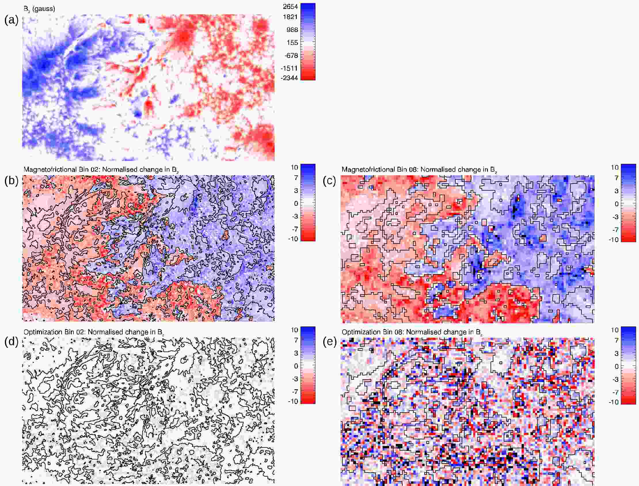
Figure 9: Changes in the vertical component $B_{z}$ of the lower boundary field within the region used for the analysis in Section 3. Panel (a) shows the magnetogram values of $B_{z}$ in the bin 2 boundary data, for reference. In panels (b)–(e), the changes $\widetilde{\Delta}_{z}$ normalized by the provided uncertainties in $B_{z}$ are displayed for two bin levels for both the magnetofrictional method in panels (b) and (c) and for the optimization method in panels (d) and (e). In panels (b) and (d), the contours correspond to the magnetogram values of $B_{z}$ shown in panel (a).

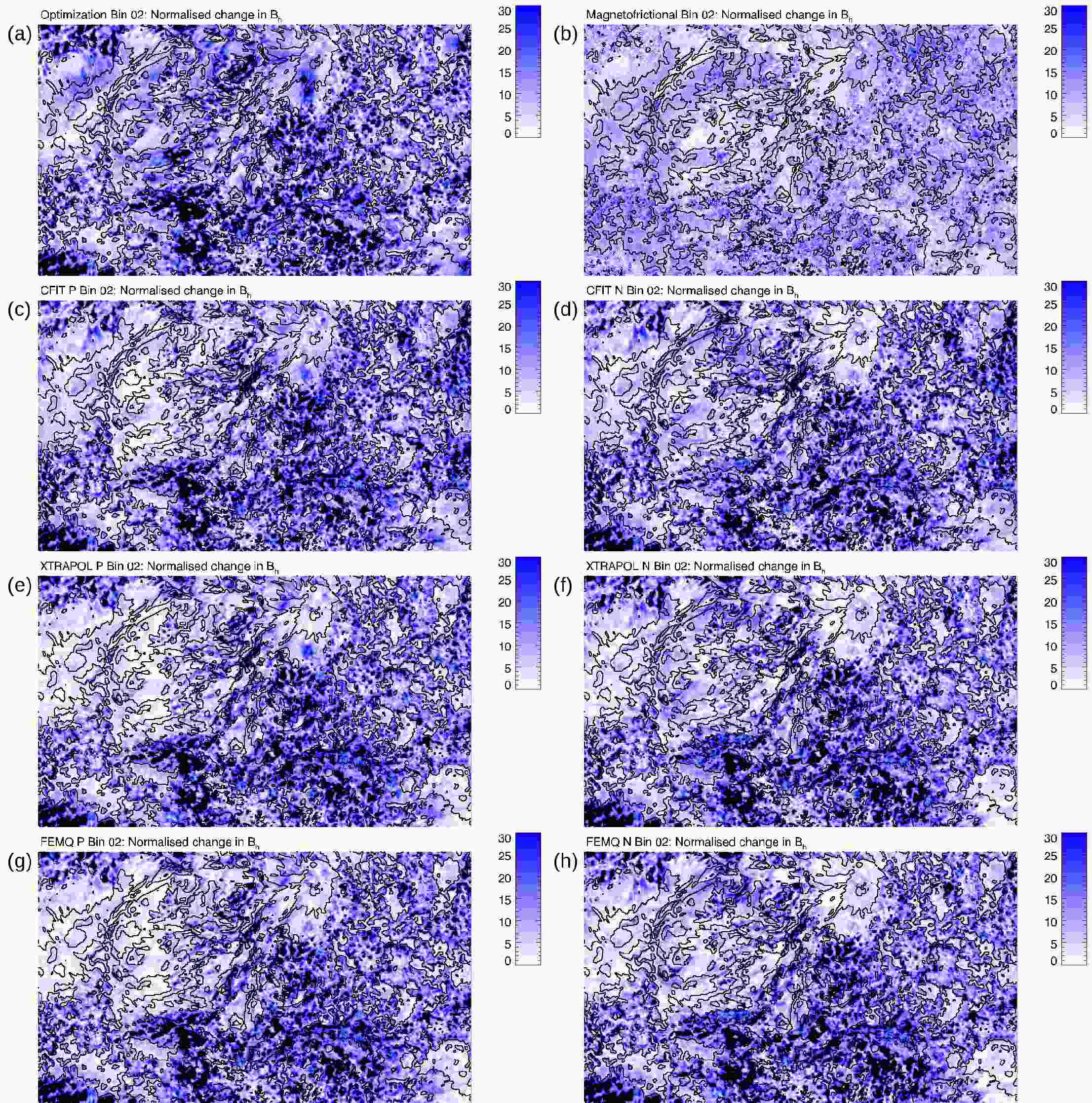
Figure 10: Changes in the magnitude $B_{h}$ of the horizontal components of the lower boundary field, for all bin 2 calculations. Panels (a) and (b) show the normalized changes for the optimization and magnetofrictional methods. The remaining panels show both the $P$ and $N$ solutions for all three Grad-Rubin codes, with panels (c) and (d) for CFIT, panels (e) and (f) for XTRAPOL, and panels (g) and (h) for FEMQ. All changes are normalized by the provided uncertainties in the horizontal components of $\boldsymbol{B}$. Contours of $B_{z}$ are overplotted for reference.

3.2 Changes to the Boundary Data

All of the solution methods introduce significant changes to the vector magnetogram boundary conditions, either initially, and/or during solution of the NLFFF equations. The magnitude of the changes are based on the uncertainties associated with the remapped vector magnetogram data, and thus tend to be more significant in weak-field regions than in regions of stronger field. Here, we characterize these changes by directly comparing the values of $\boldsymbol{B}$ on the lower boundary of the resultant NLFFF solutions to the values of $\boldsymbol{B}$ supplied by the vector magnetogram boundary data.

For each solution we define the change $\boldsymbol{\Delta}$ in the vector field at $z=0$ as

$${\boldsymbol{\Delta}}={\boldsymbol{B}}-{\boldsymbol{B}}^{\text{VM}},$$ (7)

comparing the solution $\boldsymbol{B}$ with the disambiguated vector magnetogram value $\boldsymbol{B}^{\text{VM}}$. The normalized change $\widetilde{\boldsymbol{\Delta}}$ accounts for the uncertainties $\sigma_{i}$ in each component $i$, such that

$$\widetilde{\boldsymbol{\Delta}}=\widetilde{\boldsymbol{B}}-\widetilde{\boldsymbol{B}}^{\text{VM}},$$ (8)

where $\widetilde{B}_{i}=B_{i}/\sigma_{i}$ and $\widetilde{B}_{i}^{\text{VM}}=B_{i}^{\text{VM}}/\sigma_{i}$, for each component $i=\{x,y,z\}$. We consider separately the magnitudes of the vertical components of the changes ($\Delta_{z}$ and $\widetilde{\Delta}_{z}$), and the magnitudes of the horizontal components of the changes, defined by ${\Delta}_{h}=|(\Delta_{x},\Delta_{y})|$ and $\widetilde{\Delta}_{h}=|(\widetilde{\Delta}_{x},\widetilde{\Delta}_{y})|/\sqrt{2}$, with the factor of $\sqrt{2}$ introduced so that the expected value for normalized changes in the horizontal field, taking into account its uncertainties, is unity.

Table 3 lists root-mean-square (rms) values for the magnitudes of the vertical and horizontal components of the changes in the boundary conditions defined by Equations (7) and (8) for all solutions, for boundary points within the footprint of the analysis volume $\mathcal{V}$. In calculating the rms values for the normalized changes, boundary points with assigned uncertainties less than 1 G have the uncertainty replaced by a value of 1 G. This step prevents the small uncertainties biasing the rms values.

The table shows that all methods introduce changes in the horizontal field boundary values substantially larger than the uncertainties assigned to the vector magnetogram data. In absolute units, the magnitude $\Delta_{h}^{\text{rms}}$ of the changes in the horizontal field are largely similar (several hundred Gauss) for the different methods. The magnetofrictional method introduces the smallest changes, with rms values of order 230 G to 240 G, and the other methods introduce changes which are larger by about 50%. In a normalized sense, any resolution dependence on $\widetilde{\Delta}_{h}^{\text{rms}}$ appears weak. The Grad-Rubin methods show no substantial difference in the values of $\widetilde{\Delta}_{h}^{\text{rms}}$ for the $P$ and $N$ solutions.

In addition, the optimization and magnetofrictional methods introduce changes in the vertical field, as is evident from Table 3. As with the horizontal field changes, these also exceed the uncertainties. In absolute units, $\Delta_{z}^{\text{rms}}$ for the optimization method decreases from about 160 G when using more coarsely resolved boundary data to about 30 G when more finely resolved data are used. Similarly, there is a clear trend in the normalized change $\widetilde{\Delta}_{z}^{\text{rms}}$, which is found to decrease from a factor of 7.89 when the coarsest boundary data are used to 1.17 for the data with the highest resolution. The magnetofrictional method consistently makes adjustments between 80 G and 85 G for all resolution levels. As with the optimization method, the normalized changes $\widetilde{\Delta}_{z}^{\text{rms}}$ for the magnetofrictional method trend smaller as more highly resolved data are used, ranging from 4.77 for the bin 16 data to 3.43 for the bin 2 data. By design, the Grad-Rubin methods (CFIT, XTRAPOL, and FEMQ) preserve the values of the vertical field on the boundary and thus there are no changes to the vertical components.

For the magnetofrictional method, the changes in the boundary values are introduced by the preprocessing applied to the boundary data, prior to the NLFFF calculation. The changes are comparable to the maximum values allowed by the preprocessing (see Section 2.2.2). The specific method of preprocessing used constrains the point-wise changes in the boundary values to $\pm$100 G (for $B_{z}$), and $\pm$150 G (for $B_{x}$ and $B_{y}$). The maximum/minimum values correspond to rms values $\Delta_{z}$ = 100 G and $\Delta_{h}\approx$ 280 G. For the optimization method, changes are introduced by its version of the preprocessing, which does not impose fixed point-wise constraints, and also during the calculation, as described in Section 2.2.1.

Although the Grad-Rubin methods preserve the values of the vertical field in the boundary, they do introduce changes in the horizontal field in the initial calculation of boundary values of the force-free parameter $\alpha$. Changes are also introduced during solution of the boundary value problem (see Section 2.2.3). The boundary values of the horizontal field are ignored a priori over one polarity of the vertical field.

Figures 9 and 10 show the spatial distribution of the normalized changes $\widetilde{\Delta}_{z}$ and $\widetilde{\Delta}_{h}$ across the lower boundary. In Figure 9, the changes in the vertical component $B_{z}$ of the vector magnetogram boundary data introduced by the magnetofrictional and optimization methods are shown for both the bin 2 and bin 8 calculations. The figure indicates that the magnetofrictional method changes $B_{z}$ by similar amounts (on a normalized basis) for both resolutions, with the more highly resolved boundary changed slightly less. The sign of $\widetilde{\Delta}_{z}$ correlates with the polarity, and indicates that the magnetofrictional code systematically reduces the magnitude of $B_{z}$ across the full field of view. The optimization method, in contrast, is seen to change the more highly resolved (bin 2) case significantly less than the lower-resolution (bin 8) case, on a normalized basis, without any apparent dependence on polarity.

Figure 10 illustrates the changes introduced in the magnitude of the horizontal component $B_{h}$ of the vector magnetogram data, for all methods when using the bin 2 boundary data. This figure shows that $\widetilde{\Delta}_{h}$ is about the same for all methods, with the exception for the magnetofrictional method where it is lower by about 25% due to the limits imposed during the preprocessing step. The normalized changes in $B_{h}$ are more prominent in the lower portion of the field of view where both the values of $B_{h}$ are the weakest and the uncertainties are the highest. For the Grad-Rubin methods, while there are some differences between the $P$ and $N$ solutions in the locations of the more prominent changes to $B_{h}$, there is a good general correspondence between the different methods, for a given polarity. This is expected on the basis of the Grad-Rubin method: if the different solutions (for a given polarity) have a similar connectivity, then field lines carrying strong currents will reconnect to the boundary in the opposite polarity at similar locations, and introduce the largest changes in the horizontal field at these specific locations.

4 Discussion and Conclusions

Nonlinear force-free fields (NLFFFs) are increasingly used to model the magnetic structure in the Sun’s corona. An earlier series of studies (e.g., Schrijver et al. 2006; Metcalf et al. 2008; Schrijver et al. 2008; De Rosa et al. 2009; Wheatland & Gilchrist 2013) showed that the NLFFF solution methods regularly achieved success on fields with known solutions and with appropriate boundary conditions, but still encountered difficulties in their application of the model to solar data. In this paper we re-examine one aspect identified in De Rosa et al. (2009) believed to affect the reliability of NLFFF modeling: the influence of the spatial resolution of the boundary vector magnetogram data on the NLFFF solutions.

The boundary data used for this experiment are a sequence of vector magnetograms with different spatial resolutions constructed from a single normal-map scan in December 2007 of AR 10978 by the Hinode/SOT-SP. The vector magnetograms are produced by rebinning the observed polarization spectra by factors ranging from 2 to 16, performing a Milne-Eddington inversion on these rebinned spectra, and then resolving the 180^∘ ambiguity in each case. This processing results in vector magnetograms having a spatial resolution ranging from 0$\farcs$59 to 4$\farcs$67, a range of approximately one half to one sixteenth of the native Hinode/SOT-SP normal-map resolution. The procedure of rebinning the polarization spectra (rather than the inverted vector magnetogram data) is intended to mimic observations by spectrographs with different intrinsic resolutions. AR 10978 was a relatively small and isolated region at the time of the observation, and as a result was selected for this experiment because of the presumption that much of the current-carrying field lines lie in the volume above the Hinode field of view. The region exhibited some magnetic complexity and was flare productive.

Five different codes implementing solution of the NLFFF model with three different methods (the optimization, the magnetofrictional, and Grad-Rubin methods) are applied to the set of vector magnetogram data produced from the rebinned polarization spectra. Solutions are calculated using these data, spanning the set of spatial resolutions and (for the Grad-Rubin methods) for the two choices of polarity in the boundary conditions ($P$ and $N$) on the force-free parameter $\alpha$. Although the Hinode/SOT-SP polarization spectra were also processed at the intrinsic instrumental resolution (i.e., without any rebinning), these data proved problematic for codes and computer hardware due to the size (in pixels) of the modeling domain and the corresponding time to completion, and thus we report only on the results for the boundary data at bin levels 2 to 16. In total, 71 different solution data cubes are examined.

Considered as a group, the physical quantities of interest of the NLFFF solutions span a wide range. As calculated within the common volume $\mathcal{V}$ chosen for analysis, estimated total energies $E$ range from 1.08–1.50$\times$10${}^{\text{26}}$ J, estimated free energies $E_{f}$ range from 2% to 24% of the potential field energies, and estimated relative magnetic helicities $H_{m}$ range from –0.92$\times$10${}^{\text{26}}$ Wb${}^{\text{2}}$ to 5.2$\times$10${}^{\text{26}}$ Wb${}^{\text{2}}$. The broad ranges in these estimates of physical quantities are affected by several factors. The three most significant factors are as follows:

1. The input vector magnetogram data exhibit differences across the resolution levels, as shown in Section 2.1. As a result, some variation in the subsequent NLFFF extrapolations, the lower bounds of which are constrained by the vector data, is expected. The most general trend in the results is that as the spatial resolution of the boundary data increases, the NLFFF metrics improve. In particular, using more highly resolved boundary data usually results in NLFFF solutions that are both more force- and divergence-free, as found by calculating the metrics $\left<\text{CW}\sin\theta\right>$, $\left<|f_{i}|\right>$, and $\xi$, as well as by performing the Helmholtz decomposition discussed in Section 3.1. Additionally, improvement in the NLFFF metrics is correlated with larger $E_{f}$ in most instances. Measurements of $H_{m}$, on the other hand, do not show any discernible trends with spatial resolution. Although values of $H_{m}$ from most methods agree to within a factor of two (excepting the optimization method, for which values of $H_{m}$ are clustered around zero), the lack of any trend with resolution suggests that $H_{m}$ is difficult to determine from NLFFF solutions.

2. Vector magnetogram data determined from photospheric spectral lines are not force-free, and thus are not immediately applicable to NLFFF modeling. As a result, the NLFFF extrapolation codes necessarily change the provided vector boundary data to be more compatible with the NLFFF model, resulting in boundary data that are in a more force-free state, much as what is expected at the base of the corona. The measurement uncertainties provided with the data are used to guide how these changes at the boundary occur, and changes to the field (particularly the horizontal components) are substantial when compared with the specified uncertainties, even when higher spatial resolution boundary data are used (though the specified uncertainties may be underestimates of the true uncertainties), as discussed in Section 3.2. Different extrapolation codes implement the changes in different ways, resulting in solutions from the different codes, while qualitatively similar in appearance (e.g., as in the field-line renderings of Fig. 5), that have quantitatively different characteristics (e.g., the energy estimates shown in Fig. 6).

3. Variations from method to method in the cases presented here may be as large as the effects of spatial resolution. For example, the optimization and magnetofrictional methods typically contain about 2 to 5 times more free energy than the group of Grad-Rubin methods. These variations result from a combination of effects, including not only the different treatments of the vector magnetogram data (point 2 above), but also the different conditions imposed on the lateral and top boundaries, how unbalanced flux and currents are handled, the size of the field of view relative to the flux and current systems important for NLFFF modeling, and the presence or absence of solenoidal errors. Variations amongst methods seen in earlier NLFFF extrapolation studies (e.g., Schrijver et al. 2006; Metcalf et al. 2008; Schrijver et al. 2008; De Rosa et al. 2009) were similarly wide-ranging.

We conclude that most NLFFF solutions appear more consistent with both the force- and divergence-free conditions when more highly resolved vector magnetogram data are used. Higher resolution boundary data are associated with NLFFF solutions having larger amounts of free energy. However, the use of more highly resolved boundary data does not by itself guarantee a more internally consistent solution. From a pragmatic perspective, given the spreads in $E$, $E_{f}$, and $H_{m}$ from the series of NLFFF models shown here and past experience with constructing NLFFF solutions, we recommend that users perform the following checks before a NLFFF model is employed in a scientific setting:

1. Check metrics such as $\left<\text{CW}\sin\theta\right>$, $\left<|f_{i}|\right>$, and $\xi$ and assess the degree to which a field is force- and divergence-free. In addition, performing a Helmholtz decomposition on a NLFFF model seems to be a useful way to determine the degree to which the total and free energies in the model arise from residual errors in the divergence of $\boldsymbol{B}$. These errors may be significant and may call into question the accuracies of the free energy estimates, as shown in Section 3.1.2.

2. Additionally, either verify that there is good agreement between the modeled field lines and the resulting EUV and X-ray loop trajectories before using any estimates of physical quantities from NLFFF solutions can be relied upon, or use the observed coronal loops to place additional constraints during the NLFFF solution process.

Appendix A Energy Decomposition Details

This appendix provides more details related to the Helmholtz decomposition of the magnetic energies discussed in Section 3.1.2. Values of all components in the decomposition of the magnetic energy $E$, as defined in Equation (6), for all of the NLFFF solutions are listed in Table 4. The tilde over an energy indicates normalization with respect to the total energy, so that, e.g., $\widetilde{E}_{\text{0,s}}=E_{\text{0,s}}/E$.

There is a clear distinction in results obtained with the magnetofrictional and optimization methods, which seek to minimize departures from solenoidality during computation, and the Grad-Rubin implementations, which explicitly solve for a solenoidal (divergence-free) field. In the following discussion, we compare the non-solenoidal contributions to the total energy to the $\widetilde{E}_{\text{J,s}}$ component, because $\widetilde{E}_{\text{J,s}}$ is equivalent to the free energy $E_{f}$ in a perfectly solenoidal field and it is $E_{f}$ that holds significant physical interest.

The Grad-Rubin code solutions have non-solenoidal contributions which are, in most cases, at least one order of magnitude smaller than $\widetilde{E}_{\text{J,s}}$. The Grad-Rubin codes also show little difference in results between the $P$ and $N$ solutions. For the CFIT solutions, the calculations using the bin 4 boundary data exhibit the largest non-solenoidal contributions among the CFIT results for different resolutions, with values of $\widetilde{E}_{\text{J,ns}}$ and $|\widetilde{E}_{\text{mix}}|$ that lie above the trend established by the CFIT solutions for the other resolution levels. Excepting this case, the non-solenoidal errors decrease with increasing resolution from 21% (for bin 16 boundary data) to 1% (for bin 2 data) of the free energy $\widetilde{E}_{\text{J,s}}$. The solutions obtained with the XTRAPOL code have dominant non-solenoidal contributions from $|\widetilde{E}_{\text{mix}}|$ that decrease with increasing resolution from 33% (for bin 16 data) to 1% (for bin 2 data) of $\widetilde{E}_{\text{J,s}}$. The solutions obtained with the FEMQ code lie, on average, between the CFIT and the XTRAPOL results, except for the cases using the bin 4 and bin 6 boundary data. The FEMQ solution for bin 6 boundary data has non-solenoidal contributions of $E_{\text{J,ns}}/E_{\text{J,s}}=3\times 10^{-4}$, which are the smallest amongst all methods and bin levels. These contributions are also smaller than the non-solenoidal contribution from their corresponding potential fields.

The magnetofrictional solutions exhibit non-solenoidal contributions which are a significant fraction of the free energy in about half of the cases. For example, the case using the bin 10 boundary data shows a non-solenoidal contribution of about one third of $\widetilde{E}_{\text{J,s}}$. The non-solenoidal contributions decrease with increasing resolution down to 6% of the free energy for the case where bin 2 data are used. The magnetofrictional solutions are affected by non-solenoidal contributions with energies a significant fraction of the nominal free energy, and, on average, one order of magnitude larger than for the Grad-Rubin codes. The optimization method solutions exhibit the largest non-solenoidal contributions, and the $|\widetilde{E}_{\text{mix}}|$ term is larger than the nominal free energy $\widetilde{E}_{\text{J,s}}$ at most bin levels. The mixed term generally increases in size with resolution, from a factor of 1.16 (for bin 16 data) to a factor of 1.52 (for bin 2 data) of the nominal free energy $\widetilde{E}_{\text{J,s}}$.

The solenoidal properties of the evolutionary methods are found to improve when the relaxation parameters are adjusted. For instance, by changing the parameter $w_{d}$ in Equation (4) of Wiegelmann et al. (2012) from 1.0 to 1.5, thereby weighting the divergence term more strongly during the minimization process, the solutions obtained by the optimization method are reduced by about an order of magnitude, as illustrated in Figure 11. These solutions, however, are less force-free and have less free energy than the solutions analyzed in Section 3. For these divergence-optimized solutions, the metrics $\left<\text{CW}\sin\theta\right>$ and $E/E_{0}$ range from 0.46 to 0.52 and from 1.02 to 1.08, respectively (cf. Table 2).

In summary, the Grad-Rubin codes produce solutions with relatively small non-solenoidal contributions, which can be of order 1% of $\widetilde{E}_{\text{J,s}}$ at the highest resolution. The magnetofrictional and optimization methods exhibit significantly larger non-solenoidal contributions in energy. Because Equation (8) in Valori et al. (2013) suggests that non-solenoidal contributions are correlated with the magnitude of the current-carrying part of the field, and because the magnetofrictional and optimization method solutions have the largest free energies, it is perhaps not surprising that they are characterized by the largest non-solenoidal errors. Irrespective of this effect, further reduction of the non-solenoidal errors seems likely to increase the reliability of free energy estimates from solutions obtained with the optimization and magnetofrictional methods.

Finally, we note that the non-solenoidal mixed term $E_{\text{mix}}$ is negative in a number of the NLFFF solutions and may partially cancel $E_{\text{J,ns}}$ in Equation (6). Large, negative contributions from $E_{\text{mix}}$ can in principle lead to non-physical solutions, with negative free energy. This may occur for methods that do not explicitly impose $\boldsymbol{\nabla}\boldsymbol{\cdot}\boldsymbol{B}=0$, and especially if non-preprocessed magnetograms are used. This was the case for some of the solutions obtained with the magnetofrictional and optimization methods presented in Schrijver et al. (2008) (cf. Table 1 in that paper). In Valori et al. (2013) it is shown, for one particular case, how the large negative values of $E_{\text{mix}}$ and non-physical solutions arise (mostly) because of the inconsistency of the vector magnetogram data with the force-free equations.

Figure 11: The solenoidal decomposition for the optimization solution where reducing divergence errors is weighted more strongly than reducing the Lorentz force.

Table 4: NLFFF Magnetic Energy Decomposition

Method/Code	Bin	$\widetilde{E}_{\text{0,s}}$ ($\times$10${}^{\text{--1}}$)	$\widetilde{E}_{\text{J,s}}$ ($\times$10${}^{\text{--2}}$)	$\widetilde{E}_{\text{0,ns}}$ ($\times$10${}^{\text{--4}}$)	$\widetilde{E}_{\text{J,ns}}$ ($\times$10${}^{\text{--3}}$)	$\widetilde{E}_{\text{mix}}$ ($\times$10${}^{\text{--2}}$)
Optimization	16	8.90	4.93	4.73	2.94	05.75
	14	8.78	5.88	4.15	3.94	05.88
	12	8.48	5.38	3.37	6.03	09.21
	10	8.71	5.78	3.01	4.69	06.63
	8	8.50	6.06	1.98	4.76	08.49
	6	8.47	7.61	1.30	5.16	07.13
	4	8.29	6.69	0.76	6.66	09.75
	3	8.34	8.16	0.50	6.94	07.70
	2	8.08	7.25	0.30	9.07	11.00
Magnetofrictional	16	8.65	11.5	8.17	16.3	string0.22
	14	8.68	12.0	6.42	17.9	–0.65
	12	8.55	11.6	6.53	21.9	string0.68
	10	8.37	12.1	4.64	17.8	string2.33
	8	8.79	10.5	3.25	36.5	–2.12
	6	9.16	09.3	2.53	20.9	–3.02
	4	8.89	11.0	1.32	26.8	–2.58
	2	9.11	08.6	0.43	05.1	–0.26
CFIT ($P$ / $N$)	16	9.60 / 9.67	4.77 / 4.15	15.5string / 15.5string	1.19 / 1.18	–1.02 / –1.07
	14	9.47 / 9.66	5.97 / 4.12	11.0string / 11.1string	0.91 / 0.90	–0.88 / –0.90
	12	9.54 / 9.57	5.07 / 4.72	09.77 / 09.84	0.76 / 0.74	–0.61 / –0.64
	10	9.49 / 9.51	5.52 / 5.26	07.56 / 07.59	0.56 / 0.58	–0.53 / –0.51
	8	9.48 / 9.51	5.48 / 5.16	05.28 / 05.26	0.38 / 0.39	–0.39 / –0.36
	6	9.37 / 9.51	6.44 / 5.07	03.62 / 03.68	0.27 / 0.27	–0.25 / –0.24
	4	9.04 / 9.09	7.56 / 6.33	01.84 / 01.88	1.45 / 1.93	string1.84 / string2.55
	3	9.46 / 9.45	5.50 / 5.53	01.20 / 01.20	0.09 / 0.09	–0.09 / –0.09
	2	9.40 / 9.51	6.02 / 4.95	00.56 / 00.58	0.04 / 0.05	–0.05 / –0.05
XTRAPOL ($P$ / $N$)	16	9.78 / 9.76	3.07 / 3.31	9.47 / 9.14	4.15 / 3.80	–1.01string / –1.05string
	14	9.75 / 9.72	3.29 / 3.60	6.92 / 6.71	3.34 / 3.13	–0.890 / –0.936
	12	9.68 / 9.73	3.67 / 3.21	6.01 / 5.83	2.51 / 2.28	–0.603 / –0.615
	10	9.59 / 9.66	4.60 / 3.88	4.76 / 4.69	2.02 / 1.89	–0.560 / –0.575
	8	9.58 / 9.63	4.59 / 4.07	3.45 / 3.39	1.37 / 1.28	–0.393 / –0.389
	6	9.55 / 9.64	4.72 / 3.84	2.42 / 2.40	0.95 / 0.90	–0.281 / –0.275
	4	9.48 / 9.54	5.28 / 4.77	1.34 / 1.32	0.50 / 0.48	–0.146 / –0.149
	3	9.50 / 9.59	5.06 / 4.22	0.83 / 0.82	0.33 / 0.31	–0.101 / –0.106
	2	9.50 / 9.56	5.08 / 4.48	0.40 / 0.39	0.19 / 0.19	–0.048 / –0.050
FEMQ ($P$ / $N$)	16	9.66 / 9.67	3.35 / 3.25	9.01 / 8.68	7.97 / 7.49	–0.117 / –0.120
	14	9.73 / 9.68	3.08 / 3.53	6.92 / 6.71	4.39 / 4.15	–0.454 / –0.461
	12	9.67 / 9.67	3.45 / 3.41	5.91 / 5.71	3.92 / 3.67	–0.205 / –0.197
	10	9.59 / 9.63	4.24 / 3.79	4.75 / 4.66	3.20 / 3.05	–0.183 / –0.199
	8	9.55 / 9.63	4.68 / 3.94	3.45 / 3.39	1.76 / 1.63	–0.272 / –0.275
	6	9.53 / 9.62	4.64 / 3.75	2.44 / 2.41	2.07 / 2.04	string0.001 / –0.001
	4	9.48 / 9.57	5.18 / 4.32	1.33 / 1.32	9.48 / 9.26	string0.003 / string0.001
	3	9.49 / 9.58	5.11 / 4.28	0.83 / 0.82	3.91 / 3.72	–0.064 / –0.066
	2	9.45 / 9.54	5.51 / 4.57	0.40 / 0.39	4.45 / 4.38	string0.023 / string0.024

References

- Aly (1984) Aly, J. J. 1984, ApJ, 283, 349
- Aly (1989) —. 1989, Sol. Phys., 120, 19
- Amari & Aly (2010) Amari, T., & Aly, J.-J. 2010, A&A, 522, A52
- Amari et al. (2006) Amari, T., Boulmezaoud, T. Z., & Aly, J. J. 2006, A&A, 446, 691
- Boulmezaoud & Amari (2000) Boulmezaoud, T. Z., & Amari, T. 2000, Z. angew. Math. Phys., 51, 942
- Chandra et al. (2001) Chandra, R., Dagum, L., Kohr, D., Maydan, D., McDonald, J., & Menon, R. 2001, Parallel Programming in OpenMP (San Francisco, CA, USA: Morgan Kaufmann Publishers Inc.)
- Chodura & Schlueter (1981) Chodura, R., & Schlueter, A. 1981, Journal of Computational Physics, 41, 68
- Crouch (2013) Crouch, A. D. 2013, Sol. Phys., 282, 107
- De Rosa et al. (2009) De Rosa, M. L., Schrijver, C. J., Barnes, G., Leka, K. D., Lites, B. W., Aschwanden, M. J., Amari, T., Canou, A., McTiernan, J. M., Régnier, S., Thalmann, J. K., Valori, G., Wheatland, M. S., Wiegelmann, T., Cheung, M. C. M., Conlon, P. A., Fuhrmann, M., Inhester, B., & Tadesse, T. 2009, ApJ, 696, 1780
- del Toro Iniesta (2003) del Toro Iniesta, J. C. 2003, Introduction to Spectropolarimetry (Cambridge, UK: Cambridge University Press)
- Fuhrmann et al. (2007) Fuhrmann, M., Seehafer, N., & Valori, G. 2007, A&A, 476, 349
- Fuhrmann et al. (2011) Fuhrmann, M., Seehafer, N., Valori, G., & Wiegelmann, T. 2011, A&A, 526, A70
- Georgoulis (2012) Georgoulis, M. K. 2012, Sol. Phys., 276, 423
- Grad & Rubin (1958) Grad, H., & Rubin, H. 1958, in Peaceful Uses of Atomic Energy: Proc. Second UN International Atomic Energy Conference, Vol. 31 (Geneva: UN), 190
- Gropp et al. (1999) Gropp, W., Lusk, E., & Skjellum, A. 1999, Using MPI: Portable Parallel Programming with the Message Passing Interface, 2nd edn. (Cambridge, MA: MIT Press)
- Henney et al. (2006) Henney, C. J., Keller, C. U., & Harvey, J. W. 2006, in Astronomical Society of the Pacific Conference Series, Vol. 358, Astronomical Society of the Pacific Conference Series, ed. R. Casini & B. W. Lites, 92
- Henney et al. (2009) Henney, C. J., Keller, C. U., Harvey, J. W., Georgoulis, M. K., Hadder, N. L., Norton, A. A., Raouafi, N.-E., & Toussaint, R. M. 2009, in Astronomical Society of the Pacific Conference Series, Vol. 405, Solar Polarization 5: In Honor of Jan Stenflo, ed. S. V. Berdyugina, K. N. Nagendra, & R. Ramelli, 47
- Hoeksema et al. (2014) Hoeksema, J. T., Liu, Y., Hayashi, K., Sun, X., Schou, J., Couvidat, S., Norton, A., Bobra, M., Centeno, R., Leka, K. D., Barnes, G., & Turmon, M. 2014, Sol. Phys., 289, 3483
- Jackson (1999) Jackson, J. D. 1999, Classical Electrodynamics, 3rd edn. (New York, NY: Wiley)
- Leka & Barnes (2012) Leka, K. D., & Barnes, G. 2012, Sol. Phys., 277, 89
- Leka et al. (2009) Leka, K. D., Barnes, G., Crouch, A. D., Metcalf, T. R., Gary, G. A., Jing, J., & Liu, Y. 2009, Sol. Phys., 260, 83
- Leka et al. (2012) Leka, K. D., Barnes, G., Gary, G. A., Crouch, A. D., & Liu, Y. 2012, Sol. Phys., 276, 441
- Lites et al. (2013) Lites, B. W., Akin, D. L., Card, G., Cruz, T., Duncan, D. W., Edwards, C. G., Elmore, D. F., Hoffmann, C., Katsukawa, Y., Katz, N., Kubo, M., Ichimoto, K., Shimizu, T., Shine, R. A., Streander, K. V., Suematsu, A., Tarbell, T. D., Title, A. M., & Tsuneta, S. 2013, Sol. Phys., 283, 579
- Malanushenko et al. (2014) Malanushenko, A., Schrijver, C. J., DeRosa, M. L., & Wheatland, M. S. 2014, ApJ, 783, 102
- McClymont et al. (1997) McClymont, A. N., Jiao, L., & Mikić. 1997, Sol. Phys., 174, 191
- Metcalf et al. (2008) Metcalf, T. R., De Rosa, M. L., Schrijver, C. J., Barnes, G., van Ballegooijen, A. A., Wiegelmann, T., Wheatland, M. S., Valori, G., & McTtiernan, J. M. 2008, Sol. Phys., 247, 269
- Metcalf et al. (1995) Metcalf, T. R., Jiao, L., McClymont, A. N., Canfield, R. C., & Uitenbroek, H. 1995, ApJ, 439, 474
- Metcalf et al. (2006) Metcalf, T. R., Leka, K. D., Barnes, G., Lites, B. W., Georgoulis, M. K., Pevtsov, A. A., Balasubramaniam, K. S., Gary, G. A., Jing, J., Li, J., Liu, Y., Wang, H. N., Abramenko, V., Yurchyshyn, V., & Moon, Y.-J. 2006, Sol. Phys., 237, 267
- Mikic & McClymont (1994) Mikic, Z., & McClymont, A. N. 1994, in Astronomical Society of the Pacific Conference Series, Vol. 68, Solar Active Region Evolution: Comparing Models with Observations, ed. K. S. Balasubramaniam & G. W. Simon, 225
- Molodenskii (1969) Molodenskii, M. M. 1969, SvA, 12, 585
- Parker (1996) Parker, E. N. 1996, ApJ, 471, 485
- Régnier (2013) Régnier, S. 2013, Sol. Phys., 288, 481
- Roumeliotis (1996) Roumeliotis, G. 1996, ApJ, 473, 1095
- Scherrer et al. (1995) Scherrer, P. H., Bogart, R. S., Bush, R. I., Hoeksema, J. T., Kosovichev, A. G., Schou, J., Rosenberg, W., Springer, L., Tarbell, T. D., Title, A., Wolfson, C. J., Zayer, I., & MDI Engineering Team. 1995, Sol. Phys., 162, 129
- Schou et al. (2012) Schou, J., Scherrer, P. H., Bush, R. I., Wachter, R., Couvidat, S., Rabello-Soares, M. C., Bogart, R. S., Hoeksema, J. T., Liu, Y., Duvall, T. L., Akin, D. J., Allard, B. A., Miles, J. W., Rairden, R., Shine, R. A., Tarbell, T. D., Title, A. M., Wolfson, C. J., Elmore, D. F., Norton, A. A., & Tomczyk, S. 2012, Sol. Phys., 275, 229
- Schrijver et al. (2008) Schrijver, C. J., De Rosa, M. L., Metcalf, T., Barnes, G., Lites, B., Tarbell, T., McTiernan, J., Valori, G., Wiegelmann, T., Wheatland, M. S., Amari, T., Aulanier, G., Démoulin, P., Fuhrmann, M., Kusano, K., Régnier, S., & Thalmann, J. K. 2008, ApJ, 675, 1637
- Schrijver et al. (2006) Schrijver, C. J., De Rosa, M. L., Metcalf, T. R., Liu, Y., McTiernan, J., Régnier, S., Valori, G., Wheatland, M. S., & Wiegelmann, T. 2006, Sol. Phys., 235, 161
- Semel & Skumanich (1998) Semel, M., & Skumanich, A. 1998, A&A, 331, 383
- Skumanich & Lites (1987) Skumanich, A., & Lites, B. W. 1987, ApJ, 322, 473
- Thalmann et al. (2013) Thalmann, J. K., Tiwari, S. K., & Wiegelmann, T. 2013, ApJ, 769, 59
- Thalmann & Wiegelmann (2008) Thalmann, J. K., & Wiegelmann, T. 2008, A&A, 484, 495
- Tsuneta et al. (2008) Tsuneta, S., Ichimoto, K., Katsukawa, Y., Nagata, S., Otsubo, M., Shimizu, T., Suematsu, Y., Nakagiri, M., Noguchi, M., Tarbell, T., Title, A., Shine, R., Rosenberg, W., Hoffmann, C., Jurcevich, B., Kushner, G., Levay, M., Lites, B., Elmore, D., Matsushita, T., Kawaguchi, N., Saito, H., Mikami, I., Hill, L. D., & Owens, J. K. 2008, Sol. Phys., 249, 167
- Valori et al. (2012a) Valori, G., Démoulin, P., & Pariat, E. 2012a, Sol. Phys., 278, 347
- Valori et al. (2013) Valori, G., Démoulin, P., Pariat, E., & Masson, S. 2013, A&A, 553, A38
- Valori et al. (2012b) Valori, G., Green, L. M., Démoulin, P., Vargas Domínguez, S., van Driel-Gesztelyi, L., Wallace, A., Baker, D., & Fuhrmann, M. 2012b, Sol. Phys., 278, 73
- Valori et al. (2007) Valori, G., Kliem, B., & Fuhrmann, M. 2007, Sol. Phys., 245, 263
- Valori et al. (2010) Valori, G., Kliem, B., Török, T., & Titov, V. S. 2010, A&A, 519, A44
- Wheatland (2007) Wheatland, M. S. 2007, Sol. Phys., 245, 251
- Wheatland & Gilchrist (2013) Wheatland, M. S., & Gilchrist, S. A. 2013, J. Phys. Conf. Ser., 440, 012037
- Wheatland et al. (2000) Wheatland, M. S., Sturrock, P. A., & Roumeliotis, G. 2000, ApJ, 540, 1150
- Wiegelmann & Inhester (2010) Wiegelmann, T., & Inhester, B. 2010, A&A, 516, A107
- Wiegelmann et al. (2006) Wiegelmann, T., Inhester, B., & Sakurai, T. 2006, Sol. Phys., 233, 215
- Wiegelmann & Sakurai (2012) Wiegelmann, T., & Sakurai, T. 2012, Liv. Rev. Solar Phys., 9, 5
- Wiegelmann et al. (2012) Wiegelmann, T., Thalmann, J. K., Inhester, B., Tadesse, T., Sun, X., & Hoeksema, J. T. 2012, Sol. Phys., 281, 37