A New Diagnostic of Magnetic Field Strengths in Radiatively-Cooled Shocks

Abstract

We show that it is possible to measure Alfvénic Mach numbers, defined as the shock velocity in the flow divided by the Alfvén velocity, for low-velocity (V_shock $\lesssim$ 100 km s^-1) radiative shocks. The method combines observations of bright forbidden lines with a measure of the size of the cooling zone, the latter typically obtained from spatial separation between the Balmer emission lines and the forbidden lines. Because magnetic fields become compressed as gas in the postshock region cools, even relatively weak preshock magnetic fields can be detected with this method. We derive analytical formulae that explain how the spatial separations relate to emission-line ratios, and compute a large grid of radiatively-cooled shock models to develop diagnostic diagrams that can be used to derive Alfvénic Mach numbers in flows. Applying the method to existing data for a bright knot in the HH 111 jet, we obtain a relatively low Alfvénic Mach number of $\sim$ 2, indicative of a magnetized jet that has super-magnetosonic velocity perturbations within it.

1 Introduction

Supersonic flows are common throughout the interstellar medium and govern the dynamics of a variety of objects such as stellar jets (Frank et al., 2014) and supernovae remnants (e.g. Reynolds, 2008), and also play an important role in affecting the observed spectra in protoplanetary nebulae (Riera et al., 2003) and novae shells (Williams, 2013). In cases where shocked gas cools by radiating emission lines, line ratios provide measurements of the densities, temperatures, ionization fractions, and abundances throughout the flow (e.g. Lazendic et al., 2006). Emission line widths are a powerful way to quantify the amount of turbulence and nonthermal motions present in these objects, and high-resolution images that detect proper motion have begun to open up the time-domain, making it possible to observe shear, turbulent mixing, fluid-dynamical instabilities and cooling in real time (Hartigan et al., 2011).

This wealth of information not only defines the physical characteristics at each location in flows and helps to clarify the nature of the driving sources, but can also identify the most important atomic or plasma processes that operate in supersonic flows. For example, the presence of both a narrow and a broad velocity component in the H$\alpha$ emission at the blast wave of many supernovae remnants arises from the high cross section of charge exchange between postshock ions and neutrals (Chevalier et al., 1980). The resulting H$\alpha$ emission-line shapes constrain the velocity and orientation of the shock front, and the degree to which ion and electron temperatures are equilibrated behind the shock (Ghavamian et al., 2001). The relatively large line width associated with the narrow component points to the possibility of a cosmic-ray precursor (Raymond et al., 2011). In the case of stellar jets, H II regions visible ahead of the strongest shocks define the regime where radiative precursors begin to affect shock dynamics, and the presence of transient bright spots where shock waves intersect leads to the physics of Mach stem formation and evolution (Hartigan et al., 2011; Frank et al., 2014).

Although magnetic fields can play an important role in shocked flows on both large and small scales, especially for systems like stellar jets where the driving source is likely to be an MHD disk wind of some sort, it is difficult to infer field strengths in stellar jets directly from optical emission line spectra. Optical lines show no discernible Zeeman splitting, and emission line ratios in shocked gas are degenerate with respect to field strength in the sense that spectra from low-velocity shocks without a preshock magnetic field closely resemble those from a higher-density, higher-shock velocity object with a field (Table 7 of Hartigan et al., 1994). If a bow shock is well-resolved spatially and emits in [O III] near its apex, one can use the extent of the [O III] emission and the shape of the bow to infer the shock velocity, and the H$\alpha$ flux to determine the preshock density. With this information in hand, the observed electron densities from an emission line ratio like [S II] $\lambda$6716/$\lambda$6731 give the compression, and hence the strength of the preshock and the postshock field that is oriented in the plane of the shock (i.e., perpendicular to the normal of the shock front; Morse et al., 1992, 1993).

Most jets do not emit detectable synchrotron emission, but nonthermal radio continua have been measured in a few bright knots, which are typically unresolved spatially. Fields have also been inferred from synchrotron continuum flux levels and from polarization measurements in a few cases (Ray et al., 1997; Chrysostomou et al., 2007; Carrasco-Gonzalez et al., 2010). However, converting these measurements to an estimate of the field strength requires knowledge of the electron density in the radio-emitting region immediately behind the shock where the density is changing rapidly, and also involves assumptions about the filling factor of the gas, the degree of ionization, and the power spectrum of the electrons.

Magnetic field strengths inferred from the resolved-bow-shock method and from continuum polarization both indicate surprisingly weak fields. Morse et al. (1992, 1993) found magnetic fields of $\sim$ 30$\mu$G in the preshock gas ahead of bright bow shocks in HH 34 and HH 111. The observed compression ratio between the preshock gas and the radiating gas is $\sim$ 40 (a factor of $\sim$ 4 at the shock and another $\sim$ 10 in the cooling zone), so that the field strength is $\sim$ 1mG where forbidden lines emit at temperatures of $\sim$ 7000K. The electron densities and ionization fractions determined at that location in the postshock gas imply a total density of $\sim$ $3\times 10^{4}$ cm^-3, resulting in an Alfvén speed of only $\sim$ 10 km s^-1 in the dense cooling zone. Hence, while the magnetic signal speed is comparable to the thermal velocity within shocked knots in the flow, it is negligible compared with the bulk flow velocities of $\sim$ 300 km s^-1. Field strengths inferred from radio continuum observations of the unusually strong shocks in HH 81 are also only 100$\mu$G (Chrysostomou et al., 2007). These results are in agreement with proper motions of jets like HH 111 (oriented in the plane of the sky), where internal velocity variations on the order of 40 km s^-1 produce shocks and not magnetic waves, implying that the magnetic signal speeds in the jet are at most a few tens of km s^-1 (Hartigan et al., 2001).

Two factors help to account for the anomalously low fields observed in stellar jets. First, a pulsed flow with supersonic velocity perturbations will collect magnetic field into knots, while rarefactions in the flow stretch the field out. This effect lowers the magnetic signal speed ahead of jet knots and allows smaller velocity perturbations to form shocks that otherwise would not do so (Hartigan et al., 2007). Another way to reduce the field in the jet is to remove it by reconnection. Some evidence exists for reheating at tens of AU from the sources both from high-spatial resolution observations of optical emission lines made with HST (Hartigan & Morse, 2007), and X-ray observations of quasi-stationary knots that are offset spatially from their sources (Schneider et al., 2011). In laboratory settings, magnetic towers become kink-unstable close to their driving sources (Moser & Bellan, 2012), and the same thing happens in some numerical simulations of disk winds (Staff et al., 2015). Kink instabilities could result in reconnection as the field geometry becomes increasingly complex.

With the importance of measuring field strengths in MHD flows self-evident, it is worthwhile to revisit the subject to see whether it may be possible to improve upon optical emission-line analysis of jets. Optical emission lines make the best connection to the source of any MHD wind, because they arise within the material driven directly from the source. In contrast, molecular emission lines in these outflows are typically slower and wider, and often come from a sheath of material entrained by the jet. It has been known for almost two decades that H$\alpha$ and [S II] emit from different locations in jet shocks, with H$\alpha$ coming from collisional excitation immediately behind the shock and [S II] following in a cooling zone (Heathcote et al., 1996). Surprisingly, this observational constraint has not been used to help infer field strengths, despite the fact that even a weak preshock magnetic field affects this spatial offset in a significant way (e.g. compare models B100 and E100 in Hartigan et al., 1987).

In this work we show that the additional constraint of a spatially-resolved cooling-zone breaks the degeneracy of the line ratio information and makes it possible to estimate Alfvénic Mach numbers of radiative shock waves stellar jets directly, using only quantities that are readily observable. We discuss the physics of magnetized cooling zones in Sec. 2.1, and present a large grid of shock models and their resulting diagnostics in Sec. 2.2. Although the ideal observations have yet to be made, we collect the best available data to obtain preliminary estimates of the Alfvénic Mach number for a shock in the HH 111 jet in Sec. 3, and conclude with a short Summary section.

2 Measuring Alfvénic Mach Numbers Using Emission Line Ratios and Cooling Distances

2.1 Physics of Magnetized Cooling Zones

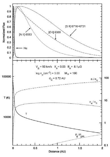
Figure 1: Structure of the cooling zone behind a typical low-velocity radiative shock. Top: Spatial distribution of radiation from several emission lines, normalized to their peak values and plotted as a function of distance from the shock. Bottom: Physical conditions in the postshock region. Temperature is read from the scale at left, and the ratios n/n_∘, n_e/n_∘, and P_B/P_gas refer to the scale at the right. Here, n_∘ is the preshock number density of nucleons, n and n_e are the number densities of nucleons and electrons, respectively, in the postshock region, and P_B / P_gas is the ratio of the magnetic pressure to gas pressure. The model parameters of V_S, X_∘, B_∘, n_∘, and M_A refer to the shock velocity, preshock ionization fraction, preshock magnetic field strength, preshock density, and incident Alfvénic Mach number, respectively. The variable d_C is the [S II]-weighted cooling-zone distance, defined in the text. This model is nonmagnetic in the sense that magnetic pressure is less than the gas pressure everywhere.

As gas enters a shock front, the pressure, temperature, and density immediately behind the shock are determined by the Rankine-Hugoniot equations, derived by balancing the mass, momentum, and energy fluxes on either side of the shock (e.g. Draine, 1993). Material that has passed through the shock is heated as the bulk kinetic energy in the flow transforms into thermal energy. The hot gas then cools by emitting line- and continuum-radiation, and within this cooling zone the temperature decreases and the density increases in response to the energy lost by radiation. The energy equation in the cooling zone of a partially-ionized steady-state shock is easily described by a formalism that relates the enthalpy per nucleus in the gas to the radiative energy loss rate (Raymond, 1979). Fig. 1 depicts an example of the spatial distribution of emission-lines in the cooling zone of a typical radiative shock front.

Several types of magnetized shocks are possible depending on the orientation of the field relative to the shock front (e.g. Chapter 7 of Gurnett & Bhattacharjee, 2005). In general, one must solve a cubic equation known as the shock adiabatic to obtain the jump conditions for density and pressure. If the field is oriented perpendicular to the shock normal (perpendicular to the velocity vector and parallel to the plane of the shock), there is a single real solution. In this case, an MHD shock forms as long as the incident velocity exceeds that of the fast magnetosonic speed V_fms = [V${}_{A}^{2}$ + C${}_{S}^{2}$]^1/2, where C_S is the sound speed in the preshock gas and V_A is the Alfvén speed in the preshock gas. If the direction of the field is aligned parallel to the normal to the plane of the shock (i.e., along the velocity vector) two solutions are possible, one where the jump conditions are the same as those of the B=0 hydrodynamical case, and another so-called switch-on shock where surface currents impart a tangential component to the field in the postshock gas.

For the general case where the field is at an angle to the surface, one can transform into the deHoffmann-Teller frame where v $\parallel$ B, and the equations have slow, intermediate, and fast solutions that correspond as the compression approaches unity to, respectively, the slow MHD wave speed, the Alfvén speed, and the fast MHD speed. Once the Alfvénic Mach number of the flow $\gtrsim$ 2, only the fast solution remains. Throughout this paper we have used the fast MHD solution, and when we refer to a magnetic field strength we mean the component perpendicular to the flow that lies in the plane of the shock. This component should be the dominant one for a typical jet geometry because in an MHD disk wind at locations far from the source, fields in jets should be mostly toroidal and therefore lie in the plane of the shock for a velocity-variable flow unless turbulence or kink instabilities randomize the direction.

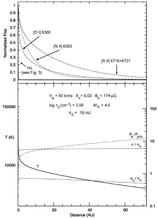
Figure 2: Same as Fig. 1 but for a stronger preshock magnetic field. The magnetic field pressure expands the cooling zone distance relative to the nonmagnetic case.

The addition of magnetic fields alters the structure of the cooling zone in important ways. Because even small ionization fractions ($\gtrsim$ 10^-4) suffice to tie the magnetic field to the gas, the magnetic field strength B is proportional to the gas density n throughout the entire cooling zone. The total pressure in the cooling zone is roughly constant, so n $\sim$ T^-1 as long as thermal motions dominate the pressure. However, the magnetic pressure B²/8$\pi$ $\sim$ T^-2, so as the temperature in the cooling zone drops, the ratio of the magnetic pressure to the thermal pressure rises, and typically exceeds unity in the forbidden-line zone (see Figs. 2, 3). Thus, even if the preshock magnetic pressure is orders of magnitude below the ram pressure at the shock front, by the time the flow radiates forbidden lines, the field usually dominates the pressure. A strong field in the cooling zone affects the observed line radiation mainly by (i) lowering the density, and (ii) by expanding the size of the cooling zone.

From an observational standpoint, one can easily measure the electron density in the cooling zone from, for example, the red [S II] ratio $\lambda$6716/$\lambda$6731, but this measurement alone does not constrain the field strength because the density in the cooling zone also depends linearly upon the preshock density. The shock velocity also matters because higher shock velocities produce hotter postshock temperatures, which result in a larger temperature drop and subsequent larger density increase once the gas reaches the forbidden line zone. In addition, the preshock ionization fraction of the gas also has a small effect on cooling zone densities because more neutral preshock conditions result in lower postshock temperatures as some of the ram energy goes into ionizing the postshock gas (Cox & Raymond, 1985). In practice, many emission lines occur in the cooling zone, and combining all of them narrows the possible parameters considerably. However, as noted in the Introduction, one cannot infer magnetic field strengths from emission line ratios alone because adding a preshock field affects emission line ratios in a similar manner to lowering the preshock density and shock velocity.

The second main observational effect of a weak preshock field - an expanded cooling zone distance - holds some promise as a diagnostic, and has not been explored completely from a theoretical or observational standpoint. In non-magnetic shocks, this distance scales approximately as a power law, V${}_{S}^{x}$n${}_{\circ}^{-1}$, where V_S is the shock velocity, n_∘ is the preshock density, and the power $x$ $\sim$ 4.0 $-$ 4.5 (Hartigan et al., 1987). Observationally, one can only measure the cooling zone size if there is an emission line that peaks at or near the location of the shock, another that peaks within the cooling zone, and this separation is resolvable with current instrumentation. Shock velocities in stellar jets are well below the threshold where radiation ionizes the preshock gas ($\sim$ 100 km s^-1), so a significant fraction of the H that enters the shock is neutral. This neutral H becomes excited by collisions at the shock and radiates strongly in Balmer emission lines in a process similar to that which produces broad and narrow Balmer filaments in some non-radiative supernova remnants (Raymond et al., 2008). Hubble images of stellar jets show that H$\alpha$ follows sharp arc-shaped features that define the locations of the shocks, while emission lines such as [S II] $\lambda$6731 follow behind these shocks with an observable spatial separation (Heathcote et al., 1996). Recent images of HH 2 show enhanced Balmer decrements (H$\alpha$/H$\beta$) at the shock fronts, as expected for collisional excitation of hydrogen (Raga et al., 2015).

Cooling zone sizes become more difficult to measure when the shock velocity is high ($\gtrsim$ 100 km s^-1), because the nature of the Balmer emission changes at higher shock velocities. Postshock temperatures in high-velocity shocks exceed $10^{6}$K, and the many different species of highly-ionized metals present at these temperatures emit energetic photons capable of ionizing H. As a result, most of the Balmer emission no longer occurs from collisional excitations of neutral H immediately behind the front, but instead originates from recombination at a secondary peak in the cooling zone where Lyman continuum photons emitted by the hot gas near the front are absorbed. In these high-velocity shocks, radiation also affects the forbidden line fluxes as electrons ejected by the Lyman continuum photons excite the low-energy states of metals by collisions. While full radiative transport is included in the models we present in Section 2.2, radiation plays almost no role in the results of this paper because, as noted above, the internal shock velocities within stellar jets derived from both emission line ratios and differential proper-motion measurements are typically $\lesssim$ 80 km s^-1 Hartigan et al. (1994).

Our models show that this secondary H$\alpha$ peak (e.g. Raga & Binette, 1991) spreads out over the same temperature range as the forbidden lines of [N II] and [S II], and its integrated flux is typically less than that of the integrated flux of the H$\alpha$ at the front as long as the preshock ionization fraction X_H $\lesssim$ 0.5. In practice, this second peak should not confuse the interpretation for most stellar jets because it lies on top of the forbidden line emission and does not appear as a distinct sharp feature. Once shock velocities exceed $\sim$ 100 km s^-1, and the preshock radiation field becomes intense enough to fully preionize the incoming gas, it will become impossible to measure cooling zone distances from H$\alpha$. However, in those cases one could in principle look for high-ionization lines such as those from N V, O VI, and C IV, or even X-ray emission to define the spatial location of the shock front and then measure this offset relative to the forbidden-line cooling zone.

Within the cooling zone there are multiple possibilities for emission-line tracers. For example, the lines of [O I] and [S II] both peak around 7000K, while those from [N II] emit on average a bit closer to the front, where T $\sim$ 10⁴K. In this paper we define a cooling zone distance d_C as the average distance from the shock of photons from the red [S II] lines $\lambda\lambda$6716+6731. In practice, this is effectively equal to the spatial offset between H$\alpha$ and [S II] because H$\alpha$ peaks immediately behind the shock. As we show in the next section, this measurement of d_C, combined with the [S II] $\lambda$6716/$\lambda$6731 flux ratio, makes it possible to infer Alfvénic Mach numbers in low-velocity radiative shocks. This method is independent of abundances and reddening, and uses the brightest emission lines in most jets. The method can be refined by including the [N I]/[N II] line ratios integrated over the cooling zone as we describe below.

Shock models in 1-D will not represent HH knots accurately if the cooling distances are a substantial fraction of the size of the shock. As we shall see in Sec. 3, cooling distances in stellar jets are typically 10 - 100 AU. The width of a typical jet at $\sim$ 0.05 pc from the source is $\gtrsim$ 1000 AU, so most HH shocks are at least an order of magnitude larger than the cooling distances. In several cases, spatial offsets between H$\alpha$ and [S II] exist along the entire extent of a well-defined shock front. Such objects are ideal for the analysis described here. Shocks that fragment into clumps $\lesssim$ 100 AU in size will be problematic to analyze with this method. Time-resolved observations of some HH knots have shown significant H$\alpha$ flux variations at the shock in response to variation in the preshock density, but the cooling zones are more stable, with flux variations on the order of factors of two over a decade and no strong evidence for variations in the line ratios there (Hartigan et al., 2011). Because our analysis relies upon integrated fluxes over the cooling zone, with H$\alpha$ used only to identify the location of the shock (H$\alpha$ intensity is not used), the assumption of steady-state is a good one as long as the shocks under consideration have had enough time to develop a full cooling zone. This cooling time is typically a decade or two, and only a handful of HH shocks are young enough for this to be a concern.

2.2 Shock Models and Diagnostic Diagrams

2.2.1 Shock Model Grid

The shock models are based on the Raymond-Cox 1-D steady-state code (Raymond, 1979). Solar-like logarithmic elemental abundances were used, H: He: C: N: O: Ne: Mg: Si: S: Ar: Ca: Fe: Ni = 12.00: 10.93: 8.52: 7.96: 8.82: 7.92: 7.42: 7.52: 7.20: 6.80: 6.30: 7.60: 6.30. The thermal and density structure of the postshock regions do not depend strongly upon the abundances, though ratios of line fluxes from different elements vary in tandem with their respective elemental abundances. The code follows the non-equilibrium distribution of all ionization states of the 13 elements listed above, and includes all the relevant atomic physics such as collisional ionization, photoionization, autoionization, recombination and dielectronic recombination, and charge exchange. We have incorporated the latest atomic parameters for Fe II given by Bautista et al. (2015) into our calculations. The models track the populations of each excited state of all the ions through a matrix of Einstein-A values and collision strengths for each transition. For example, populations in 159 levels of Fe II are derived in each time step after accounting for over 4000 emission line transitions. Radiative losses from both emission-line and continuum processes such as 2-photon radiation and bremsstrahlung are included in the energy equation to predict how the fluid variables change with time. The code employs several step sizes designed to track any regions of abrupt changes in the ionization states of the elements. We chose these as appropriate for each of the models we computed.

The radiative transfer is performed iteratively as follows. At the start of the simulation, we use a radiation field from a previous shock model with similar input parameters, and track how this spectrum is absorbed downstream in the postshock gas. Meanwhile, all the radiative emission lines are stored in an output radiation file, binned in 1.0 eV intervals beginning at 3.6 eV with 150 bins in all. At the end of the simulation the output radiation file is used as the input for the next iteration. Typically this procedure converges within two or three iterations to the final model, which predicts fluxes for all the emission lines and generates temperature, velocity, and density profiles throughout the cooling zone.

The grid consists of 8470 models. There are 11 choices for the preshock number density of nucleons n_∘ (cm^-3), with log(n_∘) = 2.0 - 4.0 in increments of 0.2. The ten choices for preshock ionization fraction X_H = n_∘(HI)/n_∘(HI + HII) of H were 0.01, 0.03, 0.05, 0.10, 0.15, 0.20, 0.30, 0.40, 0.60, and 0.80. Preshock He is neutral in all models. The shock velocity V_S had 11 values, starting at 30 km s^-1 and ending with 80 km s^-1 with increments of 5 km s^-1. Each set of (V_S, n_∘, and X_H) used seven different preshock magnetic field strengths, designed to produce Alfvénic Mach numbers M_A = V_S/V_A spaced regularly in log, with $\log_{10}$M_A = 1/6, 1/3, 2/3, 1, 4/3, 5/3 and 2 (M_A = 1.5, 2.2, 4.6, 10, 22, 46, and 100). The Alfvén speed V_A is defined by the equation V${}_{A}^{2}$ = B${}_{\circ}^{2}$/(4$\pi$n_∘m), where B_∘ is the component of the preshock magnetic field that lies perpendicular to the shock-normal, n_∘ is the preshock number density of nucleons, and m is the average mass per nucleon. Step sizes are taken to be small enough so that the temperature changes by less than 5% between steps when T $>$ 10⁴ K. Step sizes in the lower-temperature cooling zone (T $<$ $10^{4}$ K) were chosen small enough so that the uncertainties in the relevant line ratios introduced by the finite grid size were $<$ 1%. Models were terminated when the temperature fell below 2500 K. The preshock temperature was 10⁴ K in all models. This value is of little consequence in most of the models because it represents a small fraction of the kinetic energy of the flow incident upon the shock. The sound speed for mostly neutral gas at 10⁴ K is only $\sim$ 12 km s^-1.

2.2.2 Cooling Zone Emission Structure and a New Diagnostic Diagram for Magnetic Fields in Shocks

Fig. 1 displays the typical structure present in a shock with a very weak magnetic field. The gas in this 50 km s^-1 model enters the shock with a low ionization fraction of 3%, and reaches a postshock temperature of about 77000 K. Rapid cooling, due in large part to collisional excitation of neutral H, quickly drops the temperature to $\sim$ 10⁴ K after a distance of 0.1 AU, with a more gradual decline that extends over a cooling zone of $\sim$ 2 AU. The ratio of magnetic to thermal pressure rises as the gas cools, but remains less than unity throughout, so the magnetic field has no effect on the gas dynamics in this case. The density n rises as the temperature drops to keep approximate pressure balance, producing a total compression of about 70 at 2 AU, where the ionization fraction n_e/n (inferred from the separation of the dashed and dotted curves in the lower panel) is about 10%. The spatial distribution of the line emission in the upper panel shows a clear offset between H$\alpha$, which occurs at the shock, and the forbidden lines. The average distance of the [S II] emission from the front is 0.72 AU.

A magnetic case is shown in Figs. 2 and 3. In this model, the preshock magnetic field is 174 $\mu$G, which results in an Alfvénic Mach number of 4.6. The magnetic pressure dominates the gas pressure beyond about 0.1 AU, so the density remains nearly constant in the cooling zone, with a compression n/n_o of about 6, and an ionization fraction of $\sim$ 10%. This compression is much lower than in the weaker magnetic model in Fig. 1. The field reduces the immediate postshock temperature slightly relative to the nonmagnetic case, but the main difference between the two cases is that the field extends the cooling zone size by a factor of about 20. The average [S II] photon now emits at 19 AU from the shock front.

The new models are in agreement with past work (Hartigan et al., 1994) which showed that emission line ratios integrated over the entire cooling zone are degenerate with respect to field strength in the sense that line ratios from a shock with a small magnetic field resemble those from a shock with a stronger field, higher preshock density and higher shock velocity. However, when we include the cooling zone distance d_C as a constraint, and instead of the field strength we use the Alfvénic Mach number as the magnetic observable, we obtain the remarkable result shown in Fig. 4. The figure shows that different Alfvénic Mach numbers separate in a plot of the [S II] $\lambda$6716/$\lambda$6731 line ratio integrated over the cooling distance against d_C. As both the [S II] ratio and d_C are straightforward to measure for any resolved cooling zone, it is easy to use this diagram to measure M_A from observed spectra.

2.2.3 The Physics Behind the New Diagnostic

While the results displayed in Fig. 4 can be taken at face value as arising from a reliable and well-tested model that includes all the relevant physics of radiative shocks, it is a worthwhile exercise to try to understand the main physics that underlies the reason why models with different Alfvénic Mach numbers separate in Fig. 4. Let us denote the preshock gas with the subscript ‘o’, the gas immediately behind the shock with subscript ‘1’, and the point in the cooling zone where the magnetic and thermal pressures are equal with subscript ‘2’. The Alfvénic Mach number M_A is defined in terms of the shock velocity V_S, mass per nucleon m, preshock density n_o, and preshock magnetic field B_o as

$$M_{A}^{2}={{4\pi n_{o}mV_{S}^{2}}\over{B_{o}^{2}}}.$$ (1)

Equating the thermal and magnetic pressure at position 2, and using the fact that B $\sim$ n throughout the shock we obtain

$${{B_{2}^{2}}\over{8\pi}}={{B_{o}^{2}n_{2}^{2}}\over{8\pi n_{o}^{2}}}=n_{2}kT_{2}.$$ (2)

If we now make the approximation that the pressure between points 1 and 2 is constant, and employ the jump conditions for a strong shock we have

$${{B_{o}^{2}n_{2}^{2}}\over{8\pi n_{o}^{2}}}=n_{1}kT_{1}={{3n_{1}mV_{S}^{2}}\over{16}}={3\over 4}n_{o}mV_{S}^{2}.$$ (3)

Combining equations 1 and 3 we get

$$M_{A}=\sqrt{{2\over 3}}{{n_{2}}\over{n_{o}}}.$$ (4)

In the magnetic-dominated regime the density remains approximately constant because the total pressure $\sim$ B² is constant and B $\sim$ n. Hence, equation 4 implies that the compression in the forbidden-line emission zone (relative to the preshock density) is $\sim$ 1.2 M_A. For example, in Fig. 1 the compression n/n_∘ $\sim$ 6 in the forbidden emission zone, with M_A $\sim$ 5.

We now use these relations to help understand the points in Fig. 4. The y-axis of Fig. 4 is the flux ratio of [S II]$\lambda$6716/$\lambda$6731. As is well-known from ISM physics (e.g. Osterbrock & Ferland, 2006; Hartigan, 2008), there are five low-lying states for any p³ electronic configuration, and the relative populations of the ²D_5/2,3/2 states depend upon the electron density. Between the low-density limit (LDL, n_e $\sim$ 20 cm^-3) and the high-density limit (HDL, n_e $\sim$ $2\times 10^{4}$ cm^-3), I_λ6716/I_λ6731 scales roughly linearly with log₁₀(n_e), with a slope of $\sim$ $-0.5$. Assuming for the moment that cooling zones have the same ionization fractions, the y-axis in Fig. 4 becomes

$$y={{I_{\lambda 6716}}\over{I_{\lambda 6731}}}\sim{\rm constant}-0.5\,\log_{10}{n_{2}}$$ (5)

We now consider the cooling distance d_C. Let the volume emission coefficient be $\epsilon$(T) (erg cm³s^-1). Balancing the ram energy flux incident upon the shock (ignoring incident thermal and magnetic energies, which are small) with the cooling we have

$$\frac{1}{2}mn_{o}V_{S}^{3}\sim\int_{0}^{d_{C}}\epsilon(T(x))n^{2}(x)dx\sim\bar{\epsilon}\bar{n}^{2}d_{C}$$ (6)

The average emission coefficient $\bar{\epsilon}$ is a complex function of the temperature, and hence V_S, because different ionization states of different elements dominate the cooling at distinct zones throughout the shock. In the non-magnetic case when shock velocities exceed $\sim$ 100 km s^-1, numerical models show that d_C $\sim$ n${}_{\circ}^{-1}$ V${}_{S}^{q}$, where q $\sim$ 4.2 $-$ 4.6 (McKee & Hollenbach, 1980; Hartigan et al., 1987). In these shocks, the postshock temperature exceeds $10^{5}$ K, a regime where equilibrium cooling curves show that $\epsilon$ declines with T (Raymond & Smith, 1977; Schure et al., 2009). Hence, the cooling-zone volume is mostly high-temperature material, so a reasonable estimate for the average density in the volume is one that is proportional to the postshock density immediately behind shock, which in turn is a factor of four higher than the preshock density. Hence, we can estimate $\bar{n}$ to be proportional to n_∘. For $\bar{\epsilon}$ $\sim$ T^p/2 $\sim$ V${}_{S}^{p}$, equation 6 implies d_C $\sim$ n${}_{\circ}^{-1}$ V${}_{S}^{3-p}$. The numerical simulations imply an average p $\sim$ $-$1.5 for T $\gtrsim$ $10^{5}$ K, consistent with the characteristic slope for these temperatures in the equilibrium cooling curves.

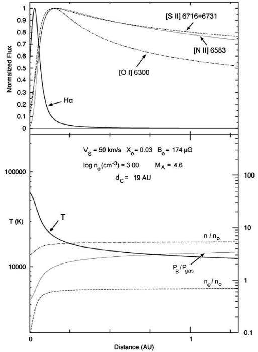
Figure 3: Same as Fig. 2 with an expanded scale on the x-axis.

The low-velocity magnetized shocks we are considering in this paper behave differently from their high-velocity non-magnetic counterparts for two reasons. First, the shock velocities are not high enough to fully preionize H. As a result, gas in low-velocity shocks cools rapidly through collisional excitation of H immediately behind the shock (Fig. 1), so that most of the gas in the cooling zone has a temperature significantly lower than that of the immediate postshock gas. Second, as shown in Figs. 2 and 3, once the magnetic pressure exceeds the thermal pressure, the gas maintains nearly a constant density while it cools. Hence, high-temperature material near the shock front occupies an even smaller fraction of the total cooling volume in the magnetized case (Fig. 2) than it does for non-magnetic low-velocity shocks (Fig. 1).

The above discussion implies that for our suite of models, the average density $\bar{n}$ in the cooling zone is approximated well by n₂, not by a constant times n_∘ as it would be in the non-magnetic case. Taking $\bar{n}$ $\sim$ n₂ and solving for d_C in equation 6 we get

$$d_{C}\sim f(V_{S})M_{A}^{-1}n_{2}^{-1}$$ (7)

where $f$(V_S) = V${}_{S}^{3}$/$\bar{\epsilon}$ is a function of the shock velocity V_S, and we have used equation 4 to relate n_o/n₂ to M_A. As above, taking $\bar{\epsilon}$ $\sim$ V${}_{S}^{p}$ and $f$(V_S) $\sim$ V${}_{S}^{3-p}$, where p is an approximate power law index gives

$$y={\rm constant}+0.5\log_{10}{d_{C}}-0.5(3-p)\log_{10}{V_{S}}+0.5\log_{10}{M_{A}}$$ (8)

Hence, models with fixed V_S and fixed M_A but different n_∘ and B_∘ follow an approximately linear curve in Fig. 4, with the higher-density models having a shorter cooling zones (d_C $\sim$ f(V_S)M${}_{A}^{-2}$n${}_{o}^{-1}$ from equations 4 and 7) and correspondingly lower I_λ6716/I_λ6731 ratios. Alternatively, if we fix V_S and d_C allow both n_o and M_A to vary, the positive sign in front of the $\log_{10}{M_{A}}$ term in equation 8 implies that models with larger M_A trend upward in Fig. 4. This is the physical reason for the color offsets in that figure. In hindsight, that the models in Fig. 4 separate when we sort by the dimensionless parameter of Alfvénic Mach number rather than by the magnetic field strength B makes sense physically because M_A determines how fast the flow is relative to the magnetic signal speed, and is the factor that determines the compression behind the shock.

The points in Fig. 4 also shift as the shock velocity V_S and the preshock ionization fraction change, but these effects are significantly smaller than the magnetic effect and effectively introduce some scatter or ‘width’ to each color band. The shock velocity term in Eqn. 8 has an opposite sign to that of the M_A term, and so affects the points in Fig. 4 in the opposite sense, in that higher values of V_S move points lower in y. For example, the groups of 5 - 10 red points that form ‘strings’ that tend down and to the right in the figure are models that have the same preshock ionization fraction, preshock density and Alfvénic Mach number, but increasing shock velocities and correspondingly higher magnetic field strengths as points trend to the lower right. Gaps between these strings of red and black points simply result from the finite number of models run.

The magnetic offsets in Fig 4 dominate over effects caused by different V_S because M_A varies by a factor of 67 in the grid, while V changes by less than a factor of 3. The models indicate that p $\sim$ 2 over the range of shock velocities in the grid, so the coefficient in front of the log₁₀ V_S term in equation 8 is essentially the same as the coefficient in front of the log₁₀ M_A term. Returning to the preshock ionization fraction, we find that it also adds a small amount of scatter to Fig. 4. Higher preshock ionization fractions imply higher electron densities and more cooling, which leads to points moving down and to the left in Fig. 4. The effective scatter introduced is $\sim$ 0.05 in I_λ6716/I_λ6731, compared with a scatter of $\sim$ 0.08 caused by varying V_S. The scatter is somewhat higher at lower M_A.

2.2.4 Improving the Diagnostic Diagram

Hundreds of possible choices exist for the y-axis in Fig. 4, using line ratios or some combination of line ratios. The [S II] $\lambda$6716/$\lambda$6731 ratio has several advantages in that it is independent of the reddening and elemental abundances, and is one of the brightest lines in an optical spectrum. However, as described above, degeneracies involving V_S and the preshock ionization fraction add some scatter to the plot. The [S II] ratio also compresses the points near the HDL and LDL, limiting broader applicability.

We can significantly improve upon uncertainties in estimates of M_A by adding additional line ratio measurements. Ideally, each color band in Fig 4 should be made as narrow as possible. A new line ratio is useful in reducing the scatter in M_A in Fig. 4 if there is a trend in a plot of [S II] $\lambda$6716/$\lambda$6731 ratio vs. the new ratio for a fixed range of d_C and a given M_A. Mathematically, it is the equivalent of searching for a nonzero partial derivative for a new line ratio with respect to [S II] $\lambda$6716/$\lambda$6731, keeping d_C and M_A fixed.

Keeping the constraint of bright emission lines that don’t depend upon reddening, and recognizing that we need a line ratio sensitive to the ionization, the [N II]/H$\alpha$ ratio integrated over the cooling zone emerges as a natural secondary diagnostic. With [S II] already a diagnostic of density and d_C, it is probably not too surprising that an important secondary indicator of M_A could come from [N II] $\lambda$6583. This line traces the ionization fraction of N because the N II/N I ratio is tied to that of H II/H I through a strong charge exchange coefficient in the plasma. Another ratio that showed promise was [S II] $\lambda\lambda$6716+6731/H$\alpha$.

However, the problem with [N II]/H$\alpha$, [S II] $\lambda\lambda$6716+6731/H$\alpha$, and similar ratios that involve different elements is that they depend linearly upon the elemental abundance ratios. These ratios are typically unknown in star-forming regions, and there is even evidence that gas-phase abundances of some elements vary along stellar jets as dust grains are destroyed (Giannini et al., 2004). Abundance ratios that use different ionization stages of the same element avoid this problem, but unfortunately there are no bright [S I] or [S III] lines to complement [S II] in most stellar jets, and one cannot easily use [O I]/[O II] either because the brightest [O II] lines ($\lambda\lambda$3727+3729) are in the blue and subject to large and poorly-known reddening corrections, and the red [O II] doublet lines at $\sim$ $\lambda$7325 are typically faint and often blended with a [Ca II] line (e.g. Brugel et al., 1981). One promising line ratio remains: [N I] $\lambda\lambda$5198+5200 / [N II]$\lambda\lambda$6548+6584, which we henceforth designate simply as ‘N I/N II’. These [N I] and [N II] lines are typically bright in HH jets, differential reddening corrections are small, and abundance uncertainties are not an issue.

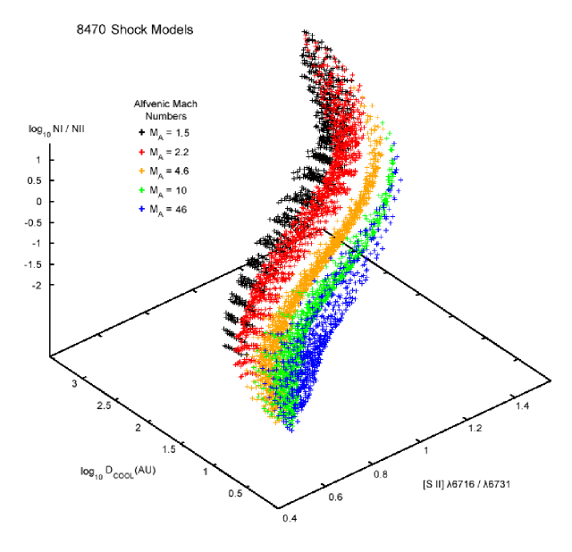
Figure 5: Same as Fig. 4 but adding in a third dimension N I/N II, defined as [N I] $\lambda\lambda$5199+5201/[N II] $\lambda\lambda$6548+6583. Models with fixed M_A trace nearly parallel sheets.

We can visualize the the constraints of additional line ratios geometrically by plotting them along a third dimension. In this case we rotate the cube of ($\log_{10}$d_C, [S II] $\lambda$6716/$\lambda$6731, and N I/N II) values in such a way as to achieve maximum separation between surfaces of constant M_A. Fig. 5 shows that models with constant M_A define a series of nested curved sheets that become degenerate only in the region where d_C $\lesssim$ 10 AU, a regime unresolvable spatially with existing instrumentation in any case. There are several orientations that separate the different M_A, but a particularly convenient one is when the line of sight is in the plane defined by ($\log_{10}$d_C, N I/N II) angled about 18 degrees from the N I/N II axis. This projection, which has [S II] $\lambda$6716/$\lambda$6731 along the x-axis, and a linear combination of $\log_{10}$d_C and N I/N II along the y-axis, is shown in Fig. 6. The width of the bands defining the red and orange points (M_A = 2.2 and 4.6, respectively) narrows by about a factor of two compared with Fig. 4. Most of the remaining scatter in each color arises because surfaces of fixed M_A are not planar sheets, but curve slightly at the ends (Fig. 5).

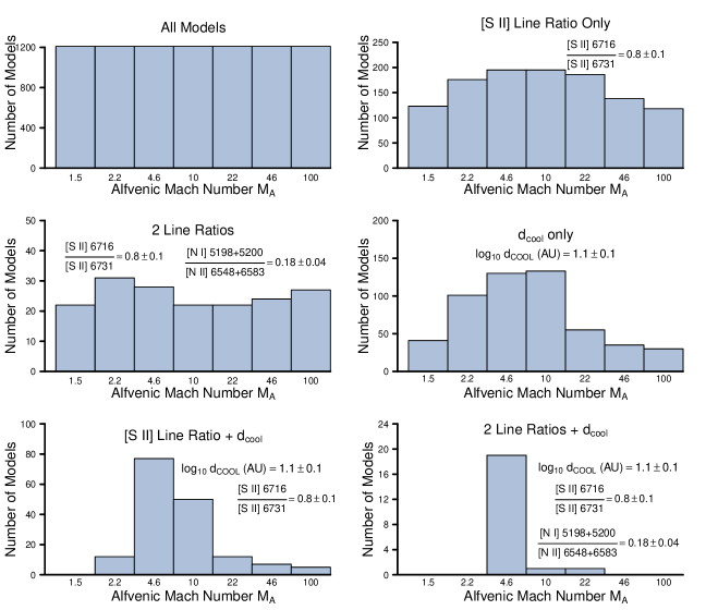
Figure 7: Histograms of the number of models satisfying the listed constraint for a hypothetical object. Alfvénic Mach numbers require both line-ratio measurements and an estimate of the cooling distance d_COOL.

Fig. 6 provides a quick way to plot a given observation on a graph and determine M_A, but given a table of models one can also simply collect all the models that are consistent with the data. As an example, Fig. 7 analyzes a hypothetical object with three observables, d_C, [S II] $\lambda$6716/$\lambda$6731, and N I/N II. A total of 1131 out of the 8470 models are consistent with the constraint [S II] $\lambda$6716/$\lambda$6731 = 0.8 $\pm$ 0.1. That number drops to 176 models once the constraint of [N I]/[N II] = 0.18 $\pm$ 0.04 is included, but the consistent models remain spread out over a range of M_A. The cooling-zone observation of $\log_{10}$ d_C = 1.1 $\pm$ 0.1 on its own limits the number of applicable models to 525, but these are again spread out over a range of M_A. It is only when the measurement of d_C is combined with the [S II] ratio (163 models) that a trend in M_A emerges, and the trend becomes a narrow range of values (21 models) once both [N II]/[N I] and the [S II] ratio are combined with d_C. One drawback with such histograms is that the number of models consistent with a given set of constraints depends upon the grid used to generate the models. Nevertheless, the peak value of the histogram always corresponds to the M_A indicated by the color plot in Fig. 6.

3 Application to Stellar Jets

While several examples of resolved cooling-zone distances have been observed with HST, images of the ratio of [S II] $\lambda$6716/$\lambda$6731 are rare, and none seem to be available for the objects like HH 111 that have relatively simple, well-defined shocks that move in the plane of the sky (which minimizes projection effects). Moreover, [N II] images are rare, and [N I] $\lambda\lambda$5198+5201 images even more rare, despite the fact that both sets of lines are easily observed in long-slit spectra.

For the purposes of this paper, we choose the isolated bow shock ‘K’ in HH 111 for further analysis (Reipurth et al., 1997). This object has a resolved cooling zone of $\log_{10}$ d_C = 1.86 $\pm$ 0.14 from archival HST images. Unfortunately, we must attempt to recover line ratios from a mixture of ground-based and space-based spectra. Long-slit STIS spectra smoothed over 0.4^′′ published by Gonzalez-Gomez & Raga (2003) indicate an electron density of 9000 cm^-3, but the S/N of the line ratio from these data is very low. From the ground, Morse et al. (1993) inferred N_e $\sim$ 600 cm^-3 near knot K, which corresponds to [S II] $\lambda$6716/$\lambda$6731 $\sim$ 1.0. However, the knot is blended to some degree with knot L, where [S II] $\lambda$6716/$\lambda$6731 $\sim$ 1.20. We adopt 1.0 for [S II] $\lambda$6716/$\lambda$6731 in knot K, but the uncertainty is rather large, $\sim$ 0.20 for this ratio. Taking the Morse et al. (1993) values integrated over knots D through J, the observed ratio of [N I] $\lambda\lambda$5198+5200 / [N II] $\lambda$6583 is 1.30, and the reddening-corrected ratio is 2.49. From the ratio of the A-values, the [N II] $\lambda$6548 flux should equal 1/3 that of [N II] $\lambda$6583. Hence, $\log_{10}$ (N I/N II) = $-$0.01 without reddening corrections, and 0.27 with reddening included. If we use the observations for knot L, then the reddening-corrected value of $\log_{10}$ (N I/N II) = 0.15. The [N I]/H$\beta$ flux ratio for knot L published by Morse et al. (1993) is in agreement with that of Noriega-Crespo et al. (1993), though we cannot use the latter reference to estimate [N II] fluxes because those spectra are only at blue wavelengths. We adopt $\log_{10}$ (N I/N II) = 0.27 $\pm$ 0.25 for knot K.

The allowed ranges for the above values define the boxed regions in Figs. 4 and 6. Despite the large uncertainties (which can be reduced significantly with dedicated observations), it is clear from both figures that the Alfvénic Mach number will lie along the lower boundary of the models, with M_A $\sim$ 1.5 $-$ 2.2. A total of 58 models yield values for d_C, N I/N II and [S II] $\lambda$6716/$\lambda$6731 consistent with the observational constraints, 25 with M_A = 2.2 and 33 with M_A = 1.5. Hence, the magnetic field is strong enough to play an important role in the dynamics of knot K in this jet. Shock velocities, log(n_∘), B_∘, and X_H are all poorly-constrained given the relatively large observational errorbars.

4 Summary

The main point of this paper is to show that a key observable - the cooling zone distance defined by the separation of H$\alpha$ from forbidden line emission - makes it possible to infer Alfvénic Mach numbers (defined as the shock velocity divided by the preshock Alfvén speed) in low-velocity shock fronts that cool radiatively. The physics behind why the method works is straightforward and the effect is unavoidable: even a weak preshock magnetic field is compressed at the shock front and continues to rise behind the front as the gas cools and the density increases. Once the magnetic pressure becomes comparable to the thermal pressure, the cooling zone lengthens.

Observational requirements include being able to measure the spatial offset between the shock and its cooling zone, for example, from a spatial offset between H$\alpha$ and [S II], and a measure of the red [S II] emission line ratio integrated over the forbidden-line emitting zone. If the fluxes of [N I] $\lambda\lambda$5200 doublet and [N II] $\lambda$6583 line are available, the models yield increasingly more precise results. The ideal dataset has not been acquired for this type of analysis, but initial application of the procedure to a bow shock in the HH 111 stellar jet indicates a rather low Alfvénic Mach number of $\sim$ 2. This Alfvénic Mach number is relative to the shock velocities in the jet. The Alfvénic Mach number relative to the bulk flow speed will be about an order of magnitude higher.

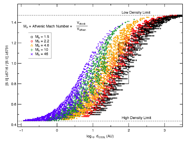
Figure 4: Different Alfvénic Mach numbers plotted as a function of two observables, the [S II]$\lambda$6716/$\lambda$6731 emission line ratio and the cooling distance, easily measured from the spatial offset between H$\alpha$ and [S II] emission. The separation of Alfvénic Mach numbers in this diagram provides a means to estimate the importance of magnetic fields in the flow dynamics. The boxed area represents current observational uncertainties for knot K in HH 111.

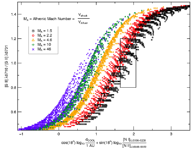
Figure 6: Same as Fig. 4 but including a correction factor to d_C that is based on the observed N I/N II ratio. This graph is the projection of Fig. 5 along a line of sight oriented 18^∘ from the N I/N II axis. The boxed region denotes the possible range of values related to knot K in HH 111.

References

- Bautista et al. (2015) Bautista, M.A., Fivet, V., Ballance, C., Quinet, P., Ferland, G., Mendoza, C., & Kallman, T.R. 2015, ApJ 808, 174
- Brugel et al. (1981) Brugel, E.W., Böhm, K.-H., & Mannery, E. 1981, ApJS 47, 117
- Carrasco-Gonzalez et al. (2010) Carrasco-Gonzalez, C., Rodriguez, L.F., Anglada, G., Marti, J., Torrelles, J.M. & Osorio, M. 2010, Science 330, 1290
- Chevalier et al. (1980) Chevalier, R., Kirshner, R.P., & Raymond, J.C. 1980, ApJ 235, 186
- Chrysostomou et al. (2007) Chrysostomou, A., Lucas, P. W., & Hough, J. H. 2007, Nature, 450, 71
- Cox & Raymond (1985) Cox, D.P., & Raymond, J.C. 1985, ApJ 298, 651
- Draine (1993) Draine, B.T. 1993, ARA&A 31, 373
- Frank et al. (2014) Frank, A., et al. in Protostars and Planets VI, H. Beuther, R. Klessen, C. Dullemond & T. Henning eds. (Tucson:Univ. of Arizona Press)
- Ghavamian et al. (2001) Ghavamian, P., Raymond, J., Smith, R.C., & Hartigan, P. 2001, ApJ 547, 995
- Giannini et al. (2004) Giannini, T., McCoey, C., Caratti o Garatti, A., Nisini, B., Lorenzetti, D., & Flower, D.R. 2004, A&A 419, 999
- Gonzalez-Gomez & Raga (2003) Gonzalez-Gomez, D.I., & Raga, A.C. 2003, RevMexAA Serie de Conf. 15, 137
- Gurnett & Bhattacharjee (2005) Gurnett, D.A., & Bhattacharjee, A. 2005, Introduction to Plasma Physics: With Space Applications, (Cambridge: Cambridge University Press)
- Hartigan (2008) Hartigan, P. 2008, Lecture Notes in Physics 742, 15-42
- Hartigan et al. (2015) Hartigan, P., Foster, J. M., Yirak, K., Liao, A.S., Graham, P., Frank, A., Wilde, B., Blue, B., Martinez, D., Rosen, P., Farley, D., & Paguio, R. 2015, in preparation
- Hartigan et al. (2011) Hartigan, P., Frank, A., Foster, J. M., Wilde, B., Douglas, M., Rosen, P., Coker, R., Blue, B., & Hansen, F. 2011, ApJ, 736, 29
- Hartigan et al. (1994) Hartigan, P., Morse, J.A., & Raymond, J.C. 1994, ApJ 436, 125
- Hartigan et al. (2001) Hartigan, P., Morse, J., Reipurth, B., Heathcote, S. & Bally, J. 2001, ApJ 559, L157
- Hartigan et al. (2007) Hartigan, P., Frank, A., Varniere, P., & Blackman, E. 2007, ApJ 661, 910
- Hartigan & Morse (2007) Hartigan, P., & Morse, J. 2007, ApJ 660, 426
- Hartigan et al. (1987) Hartigan, P., Raymond, J.C., & Hartmann, L. 1987, ApJ 316, 323
- Heathcote et al. (1996) Heathcote, S., Morse, J., Hartigan, P., Reipurth, B., Schwartz, R.D., Bally, J., & Stone, J. 1996, AJ 112, 1141
- Lazendic et al. (2006) Lazendic, J.S., Dewey, D., Schulz, N.S., & Canizares, C.R. 2006, ApJ 651, 250
- McKee & Hollenbach (1980) McKee, C.F., & Hollenbach, D.J. 1980, ARA&A 18, 219
- Morse et al. (1992) Morse, J., Hartigan, P., Cecil, G., Raymond, J., & Heathcote, S. 1992, ApJ 399, 231
- Morse et al. (1993) Morse, J., Heathcote, S., Hartigan, P., & Cecil, G. 1993b, AJ 106, 1139
- Morse et al. (1993) Morse, J., Heathcote, S., Cecil, G., Hartigan, P., & Raymond, J. 1993a, ApJ 410, 764
- Moser & Bellan (2012) Moser, A.L., & Bellan, P.M. 2012, Nature 482, 379
- Noriega-Crespo et al. (1993) Noriega-Crespo, A., Garnavich, P.M., & Raga, A.C. 1993, AJ 106, 1133
- Osterbrock & Ferland (2006) Osterbrock, D.E., & Ferland, G.J. 2005, Astrophysics of Gaseous Nebulae and Active Galactic Nuclei, (Sausalito: University Science Books)
- Raga & Binette (1991) Raga, A.C., & Binette, L. 1991, RMxA&A 22, 265
- Raga et al. (2015) Raga, A.C., Reipurth, B., Castellanos-Ramirez, A., Chiang, H.-F., & Bally, J. 2015, ApJ 798, L1
- Reipurth et al. (1997) Reipurth, B., Hartigan, P., Heathcote, S., Morse, J., & Bally, J. 1997, AJ 114, 757
- Ray et al. (1997) Ray, T.P., Muxlow, T.W.B., Axon, D.J. et al. 1997, Nature 385, 415
- Raymond (1979) Raymond, J.C. 1979, ApJS 39, 1
- Raymond & Smith (1977) Raymond, J.C. & Smith, B.W. 1977, ApJS 35, 419
- Raymond et al. (2008) Raymond, J.C., Isenberg, P.A., & Laming, J.M. 2008, ApJ 682, 408
- Raymond et al. (2011) Raymond, J.C., Vink, J., Helder, E.A., & de Laat, A. 2011, ApJ 731, L14
- Reynolds (2008) Reynolds, S.P. 2008, Ann.Rev.Astr.Ap. 46, 89
- Riera et al. (2003) Riera, A., Garcia-Lario, P., Manchado, A., Bobrowsky, M., & Estalella, R. 2003, A&A 401, 1039
- Schneider et al. (2011) Schneider, P.C., Günther, H.M., & Schmitt, J.H.M.M. 2011, A&A 530, 123
- Schure et al. (2009) Schure, K.M., Kosenko, D., Kaastra, J.S., Keppens, R., & Vink, J. 2009, A&A 508, 751
- Staff et al. (2015) Staff, J.E., Koning, N., Ouyed, R., Thompson, A., & Pudritz, R.E. 2015, MNRAS 446, 3975
- Williams (2013) Williams, R. 2013, AJ 146, 55