Inhomogeneous nuclear spin polarization induced by helicity-modulated optical excitation of fluorine-bound electron spins in ZnSe

Abstract

Optically-induced nuclear spin polarization in a fluorine-doped ZnSe epilayer is studied by time-resolved Kerr rotation using resonant excitation of donor-bound excitons. Excitation with helicity-modulated laser pulses results in a transverse nuclear spin polarization, which is detected as a change of the Larmor precession frequency of the donor-bound electron spins. The frequency shift in dependence on the transverse magnetic field exhibits a pronounced dispersion-like shape with resonances at the fields of nuclear magnetic resonance of the constituent zinc and selenium isotopes. It is studied as a function of external parameters, particularly of constant and radio frequency external magnetic fields. The width of the resonance and its shape indicate a strong spatial inhomogeneity of the nuclear spin polarization in the vicinity of a fluorine donor. A mechanism of optically-induced nuclear spin polarization is suggested based on the concept of resonant nuclear spin cooling driven by the inhomogeneous Knight field of the donor-bound electron.

I Introduction

The hyperfine interaction between electron and nuclear spins in semiconductor structures has been of particular interest over many years Meier and Zakharchenya (1984); Kalevich et al. (2008). Lately it was intensively driven by the intention to extend the electron spin coherence time and the idea to employ the nuclear spins as quantum bits (qubits) Urbaszek et al. (2013). Using optical excitation with circularly polarized light angular momentum can be transferred via the electron system to the nuclei. The polarized nuclei, in turn, act back on the electrons as an effective magnetic field (the Overhauser field), causing a splitting of the electron spin states Meier and Zakharchenya (1984). Without an external magnetic field, the hyperfine interaction with the nuclear spins is the main source of dephasing for localized electron spins in which fluctuations in the nuclear spin polarization induce fluctuations in the electron spin splittings Khaetskii et al. (2002); Merkulov et al. (2002); Dzhioev et al. (2002).

The nuclei-induced electron spin splitting can reach values of 100 $\mu$eV for high nuclear spin polarization. It can be detected spectrally as a splitting of the emission line, if the linewidth of the photoluminescence (PL) is sufficiently narrow, as it is the case for single emitters like quantum dots (QDs) or impurity centers. A relatively high nuclear spin polarization can be created using the method of optical pumping in longitudinal magnetic field (parallel to the optical axis and orthogonal to the sample surface) Brown et al. (1996); Gammon et al. (2001); Braun et al. (2006); Chekhovich et al. (2013). In the case of inhomogeneously broadened optical transitions, as it is the case in emitter ensembles, optical methods do not provide sufficient spectral resolution so that alternative approaches should be used. The nuclear spin polarization can be indirectly measured by its influence on the electron spin polarization in a transverse magnetic field, the Hanle effect Hanle (1924). In this case the Overhauser field modifies the measured degree of the circular PL polarization as a function of magnetic field applied in the direction transverse to the optical excitation Kalevich et al. (2008); Paget et al. (1977); Cherbunin et al. (2009); Auer et al. (2009); Krebs et al. (2010); Flisinski et al. (2010). If one additionally applies a polarization modulation of the excitation at a frequency corresponding to the nuclear magnetic resonance of one of the constituent isotopes, a nuclear spin polarization in the direction transverse to the optical excitation can be achieved Kalevich et al. (1980); Kalevich and Zakharchenya (1995); Cherbunin et al. (2011). However, such measurements are limited to the field ranges within the width of the Hanle curve, which is determined by the spin dephasing time of the carriers, their $g$ factor values and the nuclear spin polarization.

In the recent publication of Zhukov et al. Zhukov et al. (2014) the authors extended the magnetic field range by implementing a novel experimental technique to measure the optically-induced nuclear magnetic resonances by assessing the electron spin coherence in the resonant spin amplification (RSA) regime. For that purpose time-resolved pump-probe Kerr rotation (TRKR) was used Kikkawa and Awschalom (1998); Yugova et al. (2012). Information about the Overhauser field that changes the electron spin splitting was thereby transferred from the spectral domain into the temporal domain. In the present paper we extend the investigation of dynamic nuclear spin polarization (DNP) by applying the developed experimental approach to ZnSe doped with fluorine donors. We observe changes of the electron Larmor precession in a broad range of transverse magnetic fields, which depends on the pump power. The induced shifts of the Larmor precession change sign at the fields of the nuclear magnetic resonances (NMRs). A theoretical approach to analyze the mechanism of dynamical nuclear spin polarization for our experimental conditions is developed.

Fluorine donors in ZnSe (further ZnSe:F) and the corresponding donor-bound electron spins are currently of substantial interest because of several recent key achievements towards solid-state quantum devices: Sources of indistinguishable single photons Sanaka et al. (2009) as well as entangled photon-pairs Sanaka et al. (2012) and optically controllable electron-spin qubits De Greve et al. (2010); Kim et al. (2012); Sleiter et al. (2013) have been demonstrated so far. The spin coherence of the donor-bound electron is generally limited by the non-zero nuclear spin background in the host crystal Merkulov et al. (2002). However, in ZnSe isotopic purification can be applied to deplete the remaining low amount of non-zero nuclear spins. Apart from that, fluorine has a natural 100% abundance of spin 1/2 nuclei, which might be considered as a nuclear spin qubit coupled to a single electron spin qubit via the hyperfine interaction. These aspects make the ZnSe:F system particularly attractive for the investigation of electron and nuclear spin related features.

II Experimental details

The sample under study is a homogeneously fluorine-doped, 70-nm-thick ZnSe:F epilayer grown by molecular-beam epitaxy on a $(001)$-oriented GaAs substrate. The epilayer is separated from the substrate by a 20-nm-thick $\text{Zn}_{0.85}\text{Mg}_{0.15}\text{Se}$ barrier layer to prevent carrier diffusion into the substrate. The barrier in turn is grown on top of a thin ZnSe buffer layer to reduce the defect density at the III-V/II-VI heterointerface. The concentration of fluorine donors in the ZnSe:F epilayer is about $10^{18}$ cm^-3, so that the distance between the neighboring donors is larger than the Bohr radius of the donor-bound electrons . The sample was placed in an optical cryostat with a superconducting split-coil magnet. The sample temperature was fixed at $T=1.8$ K in all measurements.

Figure 1(a) shows the normalized PL spectrum measured for continuous-wave (cw) excitation with a photon energy of 3.05 eV. The PL is detected with a Si-based charge-coupled-device camera attached to a 0.5 m spectrometer. In the characteristic peak pattern each feature can be assigned to different exciton complexes Pawlis et al. (2006). The labels in the figure mark the following optical transitions: FX refers to the free exciton and D⁰X to the donor-bound exciton containing heavy holes (HH) or light holes (LH), respectively.

Figure 1: (a) Normalized PL spectrum measured at $B=0$ T and $T=1.8$ K. (b) Kerr rotation signal measured for resonant D⁰X-HH excitation at 2.800 eV. $B=0.5$ T. The arrow marks the negative time delay of the probe with respect to the pump at which the RSA signal is measured.

To obtain insight into the electron spin dynamics we use the TRKR technique. The electron spin coherence is generated by circularly-polarized pump pulses of 1.5 ps duration (spectral width of about 1 meV) generated by a mode-locked Ti:Sa laser operating at a repetition frequency of 75.75 MHz (repetition period $T_{\text{R}}=13.2$ ns). The laser frequency is doubled by a BBO (beta barium borate) crystal to convert the Ti:Sa range of photon energies from about $1.25-1.7$ eV to $2.5-3.4$ eV. After excitation of the sample along the growth axis z with the circularly-polarized pump pulses, the reflection of the linearly-polarized probe pulses is analyzed with respect to the angle of polarization rotation as a function of delay between the pump and probe pulses. The pump helicity is modulated between $\sigma^{+}$ and $\sigma^{-}$ circular polarization by an electro-optical modulator (EOM) using modulation frequencies $f_{\text{m}}$ in the range $20-500$ kHz. The probe beam is kept unmodulated. The Kerr rotation (KR) angle is measured with a balanced detector connected to a lock-in amplifier.

Figure 1(b) shows a TRKR signal measured at a magnetic field of $B=0.5$ T applied perpendicular to the growth axis z (Voigt geometry). Both pump and probe have the same photon energy (degenerate pump-probe scheme) and are resonant with the D⁰X-HH transition at 2.800 eV. The pump power is $P=1.1$ mW and the probe power 0.5 mW, both having a spot size of about 300 $\mu$m on the sample. The oscillations in the TRKR signal correspond to the Larmor spin precession of the donor-bound electron with a $g$ factor of $g_{\texttt{e}}=1.13\pm 0.02$. The oscillating signal at negative pump-probe delays indicates that the spin coherence is maintained up to the arrival of the next pump pulse, i.e. the electron spin dephasing time $T_{2}^{*}$ is close to the laser repetition period $T_{\text{R}}$. Due to the long spin dephasing time the action of the succeeding pump pulses on the remaining spin polarization depends on the electron $g$ factor and the magnetic field strength. In this case, the resonant spin amplification regime can be used Kikkawa and Awschalom (1998); Yugova et al. (2012) for studying spin coherence. To that end we fix the probe at a slightly negative time delay of $\Delta t=-20\,$ps with respect to the pump pulse arrival moment (see arrow in Fig. 1(b)) and detect the KR signal while scanning the transverse magnetic field. Further, we conducted experiments where an additional oscillating magnetic field (radio frequency or RF-field) $\mathbf{B}_{\mathrm{RF}}=(0,0,B_{\mathrm{RF},z})$ is applied along the $z$ axis using a small coil placed close to the sample surface.

III Experimental results

III.1 Observation of the nuclear spin polarization

Figure 2(a) shows a set of RSA curves of normalized amplitude for an EOM modulation frequency of $f_{\text{m}}=185$ kHz, measured for different pump powers. The RSA curves have the typical shape of periodic peaks as function of the magnetic field strength. The dependencies of the RSA peak distance and width on magnetic field are determined by the electron $g$ factor $g_{\texttt{e}}$, the $g_{\texttt{e}}$ spread $\Delta g$, the spin dephasing time $T_{2}^{*}$ and the repetition period of the laser pulses $T_{\text{R}}$ Kikkawa and Awschalom (1998); Yugova et al. (2012). Further optical properties of this sample and information on the electron spin dephasing and relaxation mechanisms can be found in Refs. Greilich et al. (2012); Heisterkamp et al. (2015).

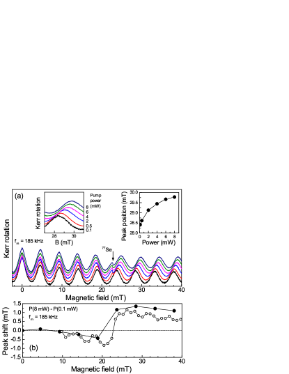
Figure 2: (Color online) (a) Normalized RSA signals measured at different pump powers and $f_{\text{m}}=185$ kHz. The NMR of ⁷⁷Se at $B=22.76$ mT is marked by the arrow. The left inset shows a close up of the RSA peaks around 29 mT. The position of the peak maximum is plotted as function of the pump power in the right inset. $T=1.8$ K. (b) Black solid circles show how the difference (shift) between the peak positions at 8 mW and at 0.1 mW from panel (a) changes in dependence on the magnetic field. Open circles demonstrate the induced shift measured directly by time-resolved KR (see text). Lines are guides to the eye.

Let us turn now to the experimental results on nuclear effects induced and detected via the spin dynamics of the resident donor-bound electrons. As mentioned above, the sample is excited by the helicity modulated pump. Under these conditions nuclear spin polarization in the system is usually suppressed, as the nuclei cannot follow the oscillating electron spin polarization fast enough due to the long nuclear spin relaxation time. However, nuclear spin polarization can be observed for finite magnetic fields in close vicinity to the NMR frequencies (corresponding to the helicity modulation frequency) of the constituent isotopes. Here the nuclear spin system becomes polarized through its cooling in the magnetic field which results from the electron spin polarization (Knight field) Knight (1949); Zhukov et al. (2014). The induced nuclear spin polarization appears in RSA curves as an additional amplitude modulation at the NMR fields, see in Fig. 2(a) the narrow resonance for the ⁷⁷Se isotope at 22.76 mT measured for $f_{\text{m}}=185$ kHz at pump powers above $0.5$ mW.

If we consider the behavior of the RSA peaks at different excitation powers we observe the following behavior: Fig. 2(a) displays several RSA curves taken at pump powers varied from $P=0.1$ mW (bottom spectrum) up to 8 mW (top spectrum). The probe power is kept in the range of $0.5$ mW for all measurements. The signal amplitudes are normalized and the curves are displaced vertically relative to each other, to simplify comparison of the peak positions. The increase of the pump power leads to a shift of the RSA peaks, which reflects a change of the electron precession frequency. The left inset in Fig. 2(a) provides a closeup of a single peak to highlight this shift. The peak positions for each curve are given in the right inset, which evidences a saturation effect at high pump powers.

One can see from Fig. 2(a), that the direction and the magnitude of the shift depend on the RSA peak position relative to the NMR field and also on the pump power. The peaks located at lower fields relative to the resonance exhibit a shift towards lower magnetic fields for increasing pump power, while the peaks at higher fields than the resonance are shifted towards higher magnetic field. The shift itself can be explained by an additional induced magnetic field acting in addition to the external magnetic field on the electron spins. The shift of RSA peaks to lower magnetic fields indicates an additional magnetic field pointing in the same direction as the external field. Vice versa, the shift to higher fields indicates opposite orientations of the induced and external fields.

To demonstrate how the peaks shift across the whole range of external magnetic fields, we plot the difference of the peak position taken at maximal (saturated, $P=8$ mW) and minimal used pump powers (0.1 mW) as a function of magnetic field. The black solid circles in Fig. 2(b) show this dependence. The circles are placed at the fields of the RSA peaks measured at minimal pump power. The induced RSA peak shift (vertical axis in Fig. 2(b)) directly corresponds to the opposite strength of the induced nuclear field.

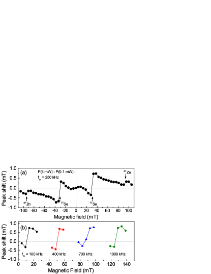
Figure 3: (Color online) (a) Induced RSA shift measured at $f_{\text{m}}=250$ kHz in a broader range of magnetic fields compared to Fig. 2. Therefore the NMR of the ⁶⁷Zn isotope is also observed. (b) Shift of the RSA peaks measured at different modulation frequencies $f_{\text{m}}$.

Figure 3(a) shows the pump induced shift over a broader range of magnetic field, measured at a modulation frequency of $f_{\text{m}}=250$ kHz. Here the NMR of the ⁷⁷Se and ⁶⁷Zn isotopes are observed at $|B|=30.75$ mT and $93.75$ mT, respectively. Figure 3(b) shows in addition the RSA shifts in the vicinity of the ⁷⁷Se NMR measured for various $f_{\text{m}}$ up to $1$ MHz. The amplitude and the shape of the shifts remain unchanged in this field range.

The dependencies in Figs. 2(b) and 3 exhibit several peculiarities:

• They show a characteristic dispersive shape around the NMRs of the constituent isotopes. In Fig. 3(a) one sees these resonance-like dispersive features for both the selenium and zinc isotopes. In the following we will call them resonances for simplicity.

• The resonances occur at magnetic fields, which are much larger than the width of the Hanle curve. Here the Hanle-curve width is given by the width of the RSA peak around zero magnetic field and is about 2 mT (full width half maximum - FWHM), see also Ref. Zhukov et al. (2014).

• The resonances are extended over a quite broad magnetic field range as result of their slowly decaying dispersive tails.

For a deeper understanding, the open circles in Fig. 2(b) show the results of additional measurements, where the induced nuclear fields are not only given at the RSA peak positions, but are also determined in between the peaks to obtain a higher resolution on magnetic field. To provide these data we determine the electron precession frequency from a measurement of the KR signal as a function of the time delay between pump and probe pulses (see Fig. 1(b)). We perform the measurements for transverse magnetic fields varied from 10 mT up to 40 mT using a 1 mT incremental step. Each data point represents the difference of the electron Larmor frequencies measured at 8 mW and 0.1 mW pump power. Using the electron $g$ factor $g_{\texttt{e}}=1.13$, one can convert this Larmor frequency difference to a magnetic field, which corresponds to the RSA peak shift, so that we can present it on the same scale as the RSA measurements.

One sees that the experimental data given by the open circles in Fig. 2(b) follow closely the solid circles. Both curves show a slight vertical shift to positive values. The FWHM of the broad dispersive resonance is on the order of 40 mT. The high resolution of the open circles data is particularly advantageous for the transition region slightly above 20 mT where the sign reversal of the RSA peak shift takes place. This sign reversal occurs in a field range of $1-2$ mT only. Note that the long tails and the sharp transition cannot be explained by a simple dispersive curve with a large homogeneous linewidth, which will be addressed in more detail by our model considerations in Sec. IV.1. Additionally, one can see that the open circles data exhibit oscillations with a period equal to the period of the RSA peaks. These oscillations could not be resolved in the data set given by the closed circles, as there the measurements were performed only at the RSA peak positions.

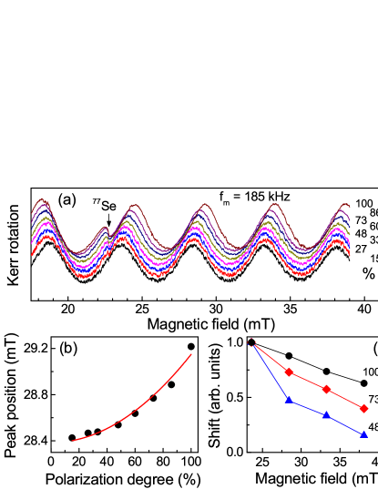
Figure 4: (Color online) (a) Normalized RSA spectra for different circular polarization degrees of the pump. The spectra are shifted vertically relative to each other for clarity. $T=1.8$ K, $P=8$ mW. (b) Position of the RSA peak around 28 mT field strength in dependence on the degree of circular polarization. Red line is a parabolic fit to the data demonstrating the quadratic dependence of the nuclear spin polarization on the circular polarization. (c) Relative peak shifts for different circular polarization degrees in dependence on the magnetic field. The data are normalized to the shift of the peak at 24 mT.

III.2 Electron spin polarization

Before we turn our attention to the investigation of the peculiarities listed in the previous section, we check how the induced nuclear spin polarization depends on the electron spin polarization. Figure 4(a) shows the measured RSA signals for several degrees of pump circular polarization at $f_{\text{m}}=185$ kHz and $P=8$ mW. The signals are normalized in amplitude to simplify comparison of the peak shift. One clearly sees for the RSA peak close to the NMR, that the pump-induced shift decreases for lower circular polarization degrees. This confirms that the nuclear spin polarization is induced by spin-oriented electrons. Figure 4(b) shows an example of the peak shift dependence on the polarization degree around 28 mT. The red line represents a parabolic fit to the data, demonstrating the quadratic dependence of the nuclear spin polarization on the degree of circular polarization.

Additionally, Fig. 4(c) shows how the peak-shift depends on the magnetic field for three different degrees of polarization. Obviously the width of the resonance is proportional to the induced nuclear spin polarization and decreases for lower polarization degrees of the electron spin. Here the shifts are given relative to the peak position for $15$% polarization degree. The shift amplitudes are then normalized to the shift of the peak at about $24$ mT. This allows us to clearly resolved the accelerated decay with magnetic field for lower degrees of the nuclear spin polarization.

For a complete understanding of the nature of the nuclear spin polarization produced by the polarized electron spins, information about the average electron spin polarization $\mathbf{S}$ is important Zhukov et al. (2014). To decide which spin component is responsible for the nuclear spin polarization we should provide a tomographic measurement for all three of them: $S_{x}$, $S_{y}$ and $S_{z}$.

III.2.1 $S_{z}$-component: Time-resolved Kerr rotation

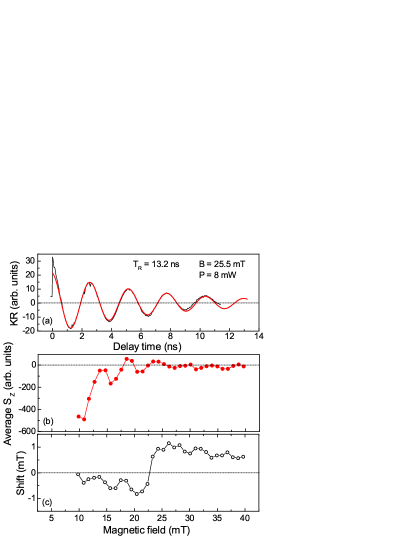
Figure 5: (Color online) (a) Example of a time resolved pump-probe Kerr signal measured at $B=25.5$ mT (black curve). Red curve is a fit to the data with an exponentially decaying cosine function recorded over the full range of delays of $T_{\text{R}}=13.2$ ns between two pump pulses. (b) Average electron spin polarization along the $z$ axis resulting from the fitted curves as a function of magnetic field. (c) Reproduction of the data from Fig. 2(b) for simplified comparison with the data in panel (b).

In our experiment the average $S_{z}$ component, which is created along the optical excitation axis can be evaluated directly from the experimental data by integrating the KR signal over the whole time period between the pump pulses. This averaging is expected to result in a finite value of $S_{z}$ in magnetic fields for which the Larmor precession period, $T_{\texttt{L}}$, is longer than or comparable with the spin dephasing time $T^{*}_{2}$. this relation is not fulfilled in strong magnetic fields, where $T_{\texttt{L}}\ll T^{*}_{2}$, $S_{z}\approx 0$, but in the field range studied here it is perfectly valid.

Figure 5(a) demonstrates an example of the measured Kerr rotation signal in the pump-probe delay range from $0$ to $13.2$ ns at $B=25.5$ mT (black curve). To evaluate $S_{z}$, which is directly proportional to the KR amplitude, we fit the data with an exponentially decaying cosine function and integrate the fit curve over the whole period of $T_{\text{R}}=13.2$ ns. The magnetic field dependence of $S_{z}$ is given in Fig. 5(b). It has a finite value for $B<15$ mT and approaches zero for higher fields. It is instructive to compare the $S_{z}(B)$ dependence with the results of the RSA shifts shown again in Fig. 5(c). From this comparison one can conclude, that the high nuclear spin polarization, corresponding to large shifts of RSA peaks, is induced in magnetic fields, where $S_{z}$ is already zero.

III.2.2 $S_{x}$: Knight field influence

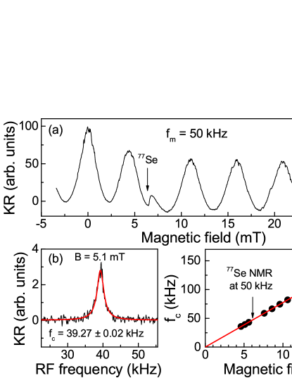
Figure 6: (Color online) (a) RSA curve measured for$f_{\text{m}}=50$ kHz at $P=8$ mW. (b) RF frequency scan at fixed $B=5.1$ mT. $f_{c}$ gives the central frequency defined by the Lorentzian fit (red curve) to the data. (c) Dependence of the $f_{c}$ on the magnetic field. Red line is a linear fit to the data.

The presence of an average electron spin polarization has an effect on the nuclei through providing an effective magnetic field, the so called Knight field, see Sec. IV.1 Meier and Zakharchenya (1984). To evaluate its value along the external magnetic field, which is proportional to $S_{x}$ spin component, one can evaluate the effect of the Knight field from the NMR frequency dependence on the magnetic field. For this purpose, we have scanned the RF-field frequency for $U_{\mathrm{RF}}=0.05$ V around the ⁷⁷Se NMR for different magnetic fields. Any Knight field component produced by an average $S_{x}$ component would induce an additional magnetic field along the $x$-axis and thereby lead to an offset of the linear dependence of NMR resonance of the ⁷⁷Se isotope on the magnetic field. Figure 6(a) shows the RSA curve measured for $f_{\text{m}}=50$ kHz at $P=8$ mW, where the ⁷⁷Se NMR is seen at about $B_{\text{NMR}}=6$ mT. Figure 6(b) gives an example of the RF-frequency scan at a fixed magnetic field of $B=5.1$ mT. As shown by the red fit using a Lorentz curve, the central NMR frequency is located at $f_{c}=39.37\pm 0.02$ kHz, showing also the precision of the measurement of the NMR position: $0.02$ kHz accuracy corresponds to about $3$ $\mu$T field strength. Finally, Fig. 6(c) represents a collection of all measured $f_{c}$ at different magnetic fields. This data set demonstrates a linear dependence of the resonance frequency with magnetic field where the corresponding fit leading to an offset of $-0.4\pm 0.2$ kHz, which corresponds to $-51\pm 26$ $\mu$T. This allows us to conclude, that the Knight field produced by a possible $S_{x}$ spin component, if present at all, should not be the reason for the measured nuclear spin polarization. As will become clear from the next sections, such an offset (or a Knight field) is negligible compared to the Knight field produced along the $y$ direction. Namely, at a distance of one localization radius $a_{l}$ from the donor center, the Knight field reaches a strength of $3.5$ mT along $y$ direction, see Sec. IV.2.

III.2.3 $S_{y}$: RF-field versus Knight field

To test the presence of a $S_{y}$ spin component we applied a RF-field with the same frequency as the used helicity modulation frequency $f_{\text{m}}$. The relative phase between this RF-field and the helicity modulation could be controlled, as well as the RF amplitude.

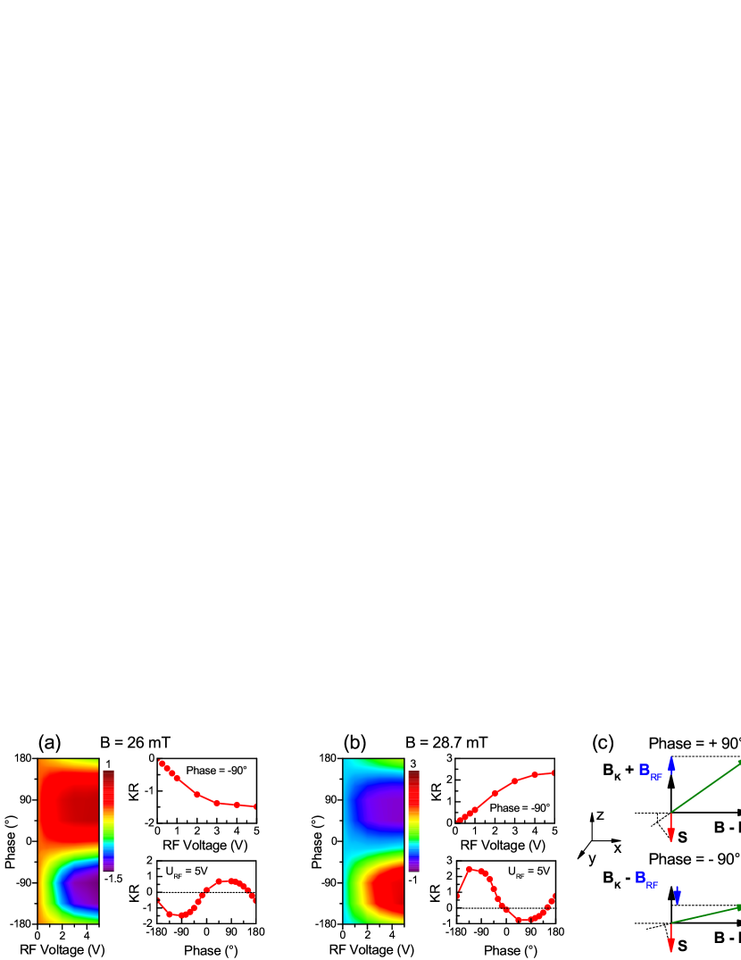
Figure 7: (Color online) (a) Contour plot for the phase between the RF field applied along the $z$ axis and the helicity modulation for different RF amplitudes at a magnetic field strength of 26 mT. On the righthand side of the plot cuts through the contour at the phase of $-90^{\circ}$ (top) and at the RF voltage of 5 V (bottom) are shown. (b) Same as in (a) but for a different magnetic field position, namely 28.7 mT. $f_{\text{m}}=185$ kHz. (c) Schemes of the rotating frame systems (RFS) for the RF field acting along the Knight field $+90^{\circ}$ and antiparallel to it $-90^{\circ}$. Both schemes are given for $B>B_{\text{NMR}}$.

In the frame system rotating with frequency $f_{\text{m}}$, one can interpret the RF-field as an additional, constant-in-time magnetic field acting on the nuclei (see Sec. IV.1 on the rotating frame system). This allow us to find the orientation of the average electron spin component and compensate its action on the nuclei by counteracting with the applied RF-field, see Fig. 7(c).

Figure 7 demonstrates the results of such measurements at different magnetic fields for $f_{\text{m}}=185$ kHz. The magnetic field values are comparable to those applied in the RSA studies Fig. 2(a). Here we plot the signal determined as the difference between the KR amplitudes with and without the RF field, applied at a fixed magnetic field for a high pump power of $P=8$ mW. Figure 7(a) shows the influence of the RF field on the KR amplitude at the field position of $B=26$ mT on the right hand side of a RSA peak, i.e. in a field range where the KR signal has a decreasing slope with increasing field. The color coding is such that blue color means reduction of the Kerr rotation signal under the influence of the applied RF-field, while red color represents an increase of the signal. The panels right next to the contour plot show cuts through the contour plot, namely the RF amplitude dependence at fixed phase of $-90^{\circ}$ (top) and the phase dependence at the saturated RF amplitude level of $U_{\mathrm{RF}}=5$ V, which corresponds to an effective magnetic field of $170$ $\mu$T (bottom) .

As one can see from the RF dependence, the Kerr amplitude is reduced for higher RF voltages, i.e. the RSA peak shifts to lower magnetic fields so that the nuclear spin polarization is reduced. This is most efficient for the phase close to $-90^{\circ}$, implying that the Knight field component should initially be oriented along the $y$ axis. In the transverse magnetic field it becomes then rotated to the direction parallel to the $z$ axis, thereby accumulating the phase of $-90^{\circ}$, which is best compensated when the RF field, applied along the $-z$ axis, is acting directly against it, see Fig. 7(c). As an additional support for this interpretation, we observe an increase of the KR amplitude at $+90^{\circ}$, where the nuclear spin polarization becomes amplified by the RF field. Here the Knight field is acting in the same direction as the RF, see Fig. 7(c), increasing therefore the overall nuclear spin projection $I_{\text{N},x}$ along the $x$-axis.

A similar behavior is observed at a higher magnetic field strength, $B=28.7$ mT, as shown in Fig. 7(b). Here we are on the left increasing slope of the next RSA peak, so that the overall amplitude changes are inverted. The RSA peak shifts to lower magnetic fields for reduced nuclear field and the KR amplitude increases. The relative phase behavior of the RF however stays the same: we reduce the nuclear spin polarization at $-90^{\circ}$ and increase it at $+90^{\circ}$, which shows that the Knight field has a constant phase shift relative to the RF field and is oriented along the $y$ axis.

Several more RSA peaks at higher magnetic fields were tested demonstrating similar behaviors (not shown here). Measurements at different magnetic fields demonstrate that the electron spin orientation stays the same. Additionally, the effect of the RF field at the phase of $-90^{\circ}$ leads to similar changes of the KR amplitude in the range of fields $20-40$ mT which has an value of about $1.9\pm 0.3$ (arb. units of KR amplitude). This means, that there is a finite average electron spin component along the $S_{y}$ direction, which stays constant when varying the transverse magnetic field strength.

IV Theoretical model and discussion

IV.1 Classical treatment

Let us consider excitation with circular polarization alternated between left and right at the modulation frequency $f_{\text{m}}$. An external magnetic field is applied perpendicular to the pump light k vector, $\textbf{k}_{\text{pump}}$, which is shine in parallel to the z axis. Figure 8(a) shows this configuration in the laboratory frame system (LFS). It is known that under helicity modulated excitation with modulation frequency $2\pi f_{\text{m}}\gg 1/T_{1}^{\text{nucl}}$ an optical polarization of the nuclear spins occurs only for $B$ close to the resonance field $B_{\text{NMR}}=2\pi f_{\text{m}}/\gamma$. Here $T_{1}^{\text{nucl}}$ is the nuclear spin relaxation time and $\gamma$ is the gyromagnetic ratio of the nuclear isotope Meier and Zakharchenya (1984); Kalevich et al. (1980). Measurements of $T_{1}^{\text{nucl}}$ will be presented elsewhere. For the studied ZnSe:F epilayer these times fall in the range of tens of milliseconds. The literature values of $\gamma$ for the ⁷⁷Se ($\gamma_{Se}=51.08\times 10^{6}$ [T s]^-1) and ⁶⁷Zn isotopes ($\gamma_{Zn}=16.77\times 10^{6}$ [T s]^-1) lead to $B_{\text{NMR}}$ [mT]$=0.123f_{\text{m}}$ [kHz] and $0.375f_{\text{m}}$ [kHz], respectively Marion (1972). These values are in very good agreement with the values observed for the NMR resonances.

In the following we consider only the ⁷⁷Se isotope having nuclear spin $I=1/2$ with an abundance $\chi=0.0758$. The hyperfine constant $A_{Se}=33.6$ $\mu$eV, which is taken for a primitive cell with two nuclei Syperek et al. (2011a, b).

The dynamic nuclear spin polarization is caused by nuclear spin flips in the presence of the electron Knight field $\mathbf{B}_{\text{K}}=b_{\text{e}}\mathbf{S}$ which precesses synchronously with the electron spin $\mathbf{S}$ and provides a temporally constant energy flow into the nuclear spin system Fleisher and Merkulov (1984). Here

$$b_{\text{e}}=-\frac{A_{Se}v_{0}}{\gamma_{Se}\hbar\pi a_{l}^{3}},$$ (1)

characterizes the maximal Knight field amplitude at the center of the donor Fleisher and Merkulov (1984). $v_{0}=a_{0}^{3}/4$ is the primitive cell volume with a two-atom basis and $a_{0}=0.566$ nm is the lattice constant of ZnSe Pawlis et al. (2011); $a_{l}$ gives the localization radius of an electron at the donor.

The average nuclear spin polarization $\mathbf{I}_{\text{N}}$ has a component along the external field $\mathbf{B}$, $I_{\text{N},x}$, and, therefore, affects the electron spin precession frequency, see Fig. 8(b). If the external magnetic field is close to the $B_{\text{NMR}}$, the projection of the nuclear field on the external field $\mathbf{B}$ is given by:

$$I_{\text{N},x}=\frac{({\mathbf{S}}\cdot\mathbf{B}_{\text{K}})(B-B_{\text{NMR}})}{(B-B_{\text{NMR}})^{2}+B^{2}_{\text{K}}+B^{2}_{\text{L}}},$$ (2)

where $B_{\text{L}}=0.006$ mT is the root mean square local field due to the nuclear dipole-dipole interactions Meier and Zakharchenya (1984); Zhukov et al. (2014).

This can be interpreted as nuclear spin cooling in the rotating frame system (RFS) Kalevich et al. (1980), see Fig. 8(b). The Knight field, oscillating with frequency $2\pi f_{\text{m}}$, can be described by a superposition of two fields, each rotating around the external field opposite to each other. Close to the NMR frequency the component, which rotates in the same direction as the nuclear spin is the important one, while the other one can be neglected. In ZnSe all nuclei have $\gamma>0$ Marion (1972), therefore this component is rotating counterclockwise if one looks in the direction along the external field B. In the RFS the electron spin is constant and the nuclei see the total magnetic field $\mathbf{B}_{\text{Total}}$, composed of the constant Knight field $\mathbf{B}_{\text{K}}$ and the effective external field $\mathbf{B}-\mathbf{B}_{\text{NMR}}$. This situation is analogous to the cooling in the laboratory frame system (LFS) in the stationary case. One can see from Eq. (2) that upon fulfilling the resonance condition $B=B_{\text{NMR}}$ the nuclear spin polarization along the external magnetic field $I_{\text{N},x}=0$.

The polarized nuclei create an Overhauser field (see Ref. Overhauser (1953)) which acts on the electron spins:

$$B_{\text{N},x}=\frac{A_{Se}{\chi}I_{\text{N},x}}{\mu_{\mathrm{B}}g_{\text{e}}}.$$ (3)

Here $\mu_{\mathrm{B}}$ is the Bohr magneton. From Eq. (2) one can see that the $B_{\text{N},x}(B)$, following $I_{\text{N},x}(B)$, has a dispersive shape. Its sign is defined by the detuning $B-B_{\text{NMR}}$. This describes exactly the behavior of the signal described in Sec. III.1, item (i).

By adding to or subtracting from the external magnetic field, the field $B_{\text{N},x}$ alters the electron spin precession frequency. In turn, this leads to a change of the electron spin polarization value at a specific external magnetic field. Usually, this effect occurs if the resonant field $B_{\text{NMR}}$ does not exceed the half width of the electron spin depolarization curve $B_{1/2}$ (Hanle curve) Kalevich et al. (1980); Cherbunin et al. (2011). Otherwise, the electrons become depolarized due to their spin precession about the transverse field $\mathbf{B}+\mathbf{B}_{\text{N},x}$, so that the value $(\textbf{S}\cdot\textbf{B}_{\text{K}})$ and the resulting $B_{\text{N},x}$ are small. Nevertheless, it has been shown in Ref. Zhukov et al. (2014) that such resonances do occur also at the $B_{\text{NMR}}$ fields, which are much stronger than $B_{1/2}$ and have a width of about one mT, see item (ii). In what follows, we concentrate on the nature of the broad resonance (item (iii)).

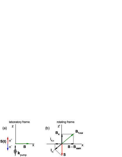
Figure 8: (Color online) (a) Spin orientation in the laboratory frame system. The red and blue arrows symbolize the electron spins generated with $\sigma^{+}$ and $\sigma^{-}$ photons, respectively, alternating in helicity with $f_{\text{m}}$. (b) Scheme of magnetic fields, acting on the nuclei in the rotating frame. The frame is rotating about the x axis with frequency $2\pi f_{\text{m}}$ in the direction of the nuclear spin precession. $\mathbf{B}_{\text{K}}$ and $\mathbf{S}$ are the average electron Knight field and spin, respectively, which are fixed in the rotating frame and are rotating with $2\pi f_{\text{m}}$ in the laboratory frame. $I_{\text{N},x}$ is the projection of the induced nuclear spin polarization onto the direction of the external field $\mathbf{B}$.

As one can see, Eqs. (2) and (3) support the measurements presented in Figs. 4(a) and 4(b). The nuclear spin polarization, which causes the RSA shift via the Overhauser field $B_{\mathrm{N},x}$, indeed follows the $S^{2}$ dependence. The $S^{2}$ dependence comes from the product $(\textbf{S}\cdot\textbf{B}_{\text{K}})$, where $\mathbf{B}_{\text{K}}=b_{\text{e}}\mathbf{S}$. The accelerated decay of the nuclear spin polarization with increased magnetic field is also well described by the $S^{2}$ dependence in the denominator of Eq. (2), see Fig. 4(c).

As mentioned before, the sign of the induced shifts in Fig. 2(b) is opposite to the induced nuclear fields, $B_{\text{N},x}$. Taking into account that in ZnSe the electron $g$ factor $g_{e}>0$, so that $b_{e}<0$ and that the hyperfine constant $A_{Se}>0$, Eq. (3) reproduces this sign dependence. It is negative for $B>B_{\text{NMR}}$ and positive vice versa.

We now try to simulate on the basis of Eq. (3) the data shown by the open circles in Fig. 2(b) and reproduced in Fig. 9. The fitting parameters in this procedure are $b_{e}$ and $S$. $S$ is fixed at $0.07$, which will be justified below. Figure 9 demonstrates examples for a homogeneous nuclear spin polarization using $b_{e}=-10$ mT and $-100$ mT, given by the red and blue curves, respectively. As can be seen, the $b_{e}=-10$ mT curve describes only the fast changeover of the sign close to the resonance very well, but completely fails to fit the data away from the resonance. On the other hand, the $b_{e}=-100$ mT curve shows the right tendency compared to the data only in the tails, far from the resonance condition. The amplitudes here, however, deviate considerably from the measured data points.

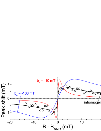
Figure 9: (Color online) Peak shift and corresponding $B_{\text{N},x}$ calculated for the ⁷⁷Se isotope after Eq. (5) (black line) with $b_{\text{e}}=-370$ mT, $S=0.07$ and $a_{l}=3.4$ nm. For comparison we show two homogeneously broadened curves calculated after Eq. (3) using $b_{\text{e}}=-10$ mT (red line) and $b_{\text{e}}=-100$ mT (blue line). Open circles represent the experimental data as in Fig. 2(b), but shifted slightly downwards to compensate for the offset.

This simulation leads to an important conclusion: the Knight field is not constant within the localization area of the donor-bound electron. As is well known, a uniform spin polarization of the nuclei can be established through spin diffusion based on flip-flop processes between the nuclei at different distances relative to the donor center Dyakonov (2008); Bloembergen (1954). Spin diffusion is allowed, if the energy is conserved (or nearly conserved) thereby, so that the energy difference between spin flips of two nuclei does not exceed $\hbar\gamma B_{\text{L}}$, and therefore, can be compensated by the dipole-dipole nuclear reservoir. In our case, however, the nuclei are exposed to an inhomogeneous Knight field $B_{\text{K}}=b_{\text{e}}(r)S=b_{\text{e}}S\exp{(-2r/a_{l})}$, which is different for neighboring nuclei and is given by the electron wave function at the donor: $\Psi^{2}(r)=(\pi a^{3}_{l})^{-1}\exp(-2r/a_{l})$. Here $r$ is the distance from the donor center. Neighboring nuclei of ⁷⁷Se are separated by a distance of about $R=a_{0}/\chi_{\text{Se}}^{1/3}=0.566/0.0758^{1/3}=1.34$ nm Greilich et al. (2012). The difference of the Knight field at neighboring isotopes is than in the order of $b_{\text{e}}S\exp{(-2r/a_{l})}[1-\exp{(-2R/a_{l})}]$. This should be compared with the local nuclear field $B_{\text{L}}\approx 0.006$ mT. Therefore the radial diffusion of the nuclear spin becomes only possible if $b_{\text{e}}S\exp(-2r/a_{l})[1-\exp(-2R/a_{l})]\leq B_{\text{L}}$. To estimate the $r$ at which the nuclear spin diffusion becomes possible, we need to know the values for $b_{e}$ and $S$.

The activation energy (or donor binding energy) of the electron bound to the fluorine donor ($E_{\text{a}}=27$ meV) allows us to estimate the localization radius of the electron $a_{l}=3.4$ nm using $a_{l}=\hbar/\sqrt{2m^{\text{eff}}_{\text{e}}}E_{\text{a}}$, with $m^{\text{eff}}_{\text{e}}=0.145m_{\text{e}}$ Greilich et al. (2012), where $m_{\text{e}}$ is the free electron mass in vacuum. This small $a_{l}$ value should lead to a significant Knight field at the donor center. Using Eq. (1) given at the beginning of the Sec. IV.1 we obtain $b_{\text{e}}=-370$ mT . Then, taking into account that $S=0.07$ (see below in this section) this leads to the result, that the nuclear spin diffusion should be hindered within a radius of about $3.9$ $a_{l}$, resulting in this range in a spatially inhomogeneous nuclear spin polarization, $I_{\text{N},x}(r)$.

Due to the spherical symmetry of the spin diffusion the polarization is also isotropic. Thus, the spatial distribution of the nuclear spin polarization is given by:

$$I_{\text{N},x}(r)=\frac{b_{\text{e}}S^{2}(B-B_{\text{NMR}})\exp{(-2r/a_{\text{l}})}}{(B-B_{\text{NMR}})^{2}+b_{\text{e}}^{2}S^{2}\exp{(-4r/a_{\text{l}})}},$$ (4)

We neglect here the small $B_{\mathrm{L}}$ fields. The polarized nuclei, in turn, act on the electrons via the Overhauser field:

$$B_{\text{N},x}=\frac{A{\chi}}{\mu_{\text{B}}g_{\text{e}}}\int I_{\text{N},x}(r)\Psi^{2}(r)4\pi r^{2}dr.$$ (5)

We use Eq. (5) to fit the experimental data for the induced nuclear field given in Fig. 9. The best fit is shown by the black curve. It has been achieved for $b_{\text{e}}=-370$ mT and an average electron spin polarization of $S=0.07$, and reproduces all features of the experimental dependence. Namely, the fast changeover of the field sign at the resonance $B_{\mathrm{NMR}}$ and the broad tails due to the widely extended decay.

Figure 10 shows schematically the behavior of the Knight field ($B_{\text{K}}=b_{\text{e}}S\exp{(-2r/a_{l})}$) and the nuclear spin polarization ($I_{\text{N},x}$) using Eq. (4) as a function of the distance from the donor. As soon as the radius becomes larger than $3.9$ $a_{l}$ spin diffusion becomes possible and equalizes the nuclear spin polarization spatially, as shown schematically by the red solid line showing the region of flat nuclear spin polarization above $3.9$ $a_{l}$.

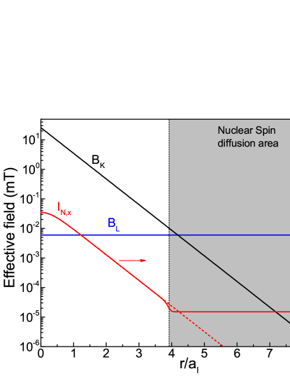
Figure 10: (Color online) Illustration of different fields as function of the distance from the donor center in units of the localization radius $a_{l}$. $B_{\text{K}}$, black line, is the Knight field. Here the simulation is done using $b_{\text{e}}S=25.9$ mT. Grey shaded area shows the region where the spin diffusion in the nuclear spin system becomes possible. $I_{\text{N},x}$, red dashed line, shows the nuclear spin polarization using $B-B_{\text{NMR}}=b_{e}S$. Red solid line represents schematically the effect of nuclear spin diffusion on $I_{\text{N},x}$, which equalizes the nuclear spin polarization spatially for $r>3.9$ $a_{l}$. Blue line shows the strength of the local fields $B_{\mathrm{L}}=0.006$ mT.

Using Figs. 9 and 10 one can draw the following qualitative conclusions: (a) close to the resonance ($B=B_{\text{NMR}}$) the electron is exposed to a very weak nuclear spin polarization produced by the Knight field far from the donor, at the edges of the nuclear spin diffusion area. As the concentration of fluorine donors in this sample is $n=1\times 10^{18}$ cm^-3, the average distance between them is $\bar{d}=\left(\frac{3}{4\pi n}\right)^{1/3}=62$ nm. This corresponds to about $18a_{l}$, so that the donors are not located in the inhomogeneous nuclei polarisation volumes of the neighbors. (b) At the center of the donor, the electrons are exposed to the strongest nuclear spin polarization produced by the maximal Knight field. This is the position far from the resonance on the magnetic field axis in the extended tails of our inhomogeneous dispersive curve in Fig. 9. A simple estimation using the integral $\int\Psi^{2}(r)4\pi r^{2}dr$ shows, that the electron is 98% confined within the volume given by the radius $3.9$ $a_{l}$. The nuclear spin polarization decreases at that distance from the donor by a factor of about 1200. If the spin diffusion border would be much closer to the donor or, with other words, if $B_{\text{L}}$ would be bigger, the extended tails would decay much faster with magnetic field. For example, in GaAs $B_{\text{L}}=0.3$ mT Fleisher and Merkulov (1984). If taking into account $b_{e}\approx 20$ mT as well as $a_{l}=10$ nm Fleisher and Merkulov (1984) and using similar considerations with $S=0.07$ as for ZnSe, one can estimate the diffusion border to be at $r\approx 0.3a_{l}$. This small borderline would give a quite homogenous nuclear spin polarization around the donor and lead to a narrow NMR resonance, experimental examples are given in Ref. Zhukov et al. (2014).

IV.2 Average electron spin polarization in external magnetic field

The next point to clarify is the value of the average electron spin polarization in the range of magnetic fields around the NMR field. These fields are much higher than the half width of the Hanle curve ($B_{1/2}$). In our simulations using Eq. (5) we have estimated the average electron spin value to be constant at $S=0.07$. The value of the average nuclear spin polarization given in Eq. (2) is proportional to $({\mathbf{S}}\cdot{\mathbf{B}_{\text{K}}})=b_{\text{e}}S^{2}(t=0)B_{1/2}^{2}/(B_{1/2}^{2}+B^{2})$ and is expected to be reduced by a factor of $(B/B_{1/2})^{2}\gg 1$ for higher magnetic fields Meier and Zakharchenya (1984). Here $(B/B_{1/2})^{2}\approx(20$ [mT]/$1$ [mT]$)^{2}=400$ and the average electron spin transverse to the magnetic field should be very small due to the Larmor precession of the electron spin about this field. This statement agrees with our experimental observations presented in Fig. 5(b) in Sec. III.2.

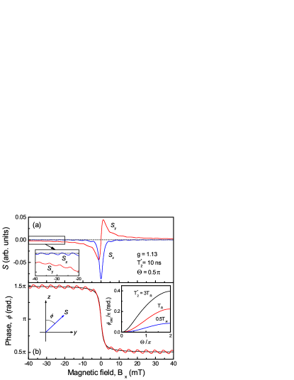
Figure 11: (Color online) (a) Evolution of the average spin components in transverse magnetic field $\mathbf{B}=(B_{x},0,0)$. Inset shows a close-up for magnetic fields from -40 to -20 mT to demonstrate the relative weights of the spin components. (b) Phase relation between the spin components. The amplitude of the oscillations in the red curve can be related to the red curve in the inset. This amplitude depends on the spin dephasing in relation to the laser repetition period, over which the averaging is done. The longer the spin dephasing takes, the smaller the amplitude that is expected for the oscillations, see black curve in the inset and panel (b).

However, the experimental observation of the broad resonance allows us to assume that there is an average electron spin polarization present in a wide range of magnetic fields, which leads to polarization of the nuclei, in particular along the external magnetic field axis, seen as $I_{\text{N},x}$ in Fig. 8(b). Using Eq. (13) of Ref. Zhukov et al. (2014) we can estimate the average electron spin polarization along the $y$ and $z$ directions, where $z$ is the optical excitation axis. The averaging is done over the period of the laser repetition, $T_{\text{R}}$. Figure 11(a) demonstrates the evolution of the average electron spin components with the transverse magnetic field, $B_{x}$. The $S_{z}$ component decays completely within a range of 10 mT (which fits well to our observations in Fig. 5), while the $S_{y}$ component is slowly decaying up to tens of mT, see the inset to panel (a) magnifying the difference at higher fields. As mentioned in Ref. Zhukov et al. (2014), the vector sum of the $z$ and $y$ spin components decays with increasing transverse field $B$ as $1/B$.

Figure 11(b) shows the corresponding evolution of the phase $\phi$ between the $S_{z}$ and $S_{y}$ spin components. It allows us to conclude, that the average spin polarization along the $y$ direction should be present and have a constant phase shift of $90^{\circ}$ relative to the $S_{z}$ component in the range of magnetic fields above 5 mT. The inset demonstrates the power dependence of the phase-oscillation amplitude present in the simulated signal for different electron spin dephasing times, $T_{2}^{*}$, in relation to the laser repetition period $T_{\text{R}}$. The red curve represents the simulation using the realistic parameters of our system, $T_{2}^{*}=10$ ns and $T_{\text{R}}=13.2$ ns. $\Theta$ is the optical pulse area, $\Theta=\int 2\langle d\rangle E(t)dt/\hbar$, where $\langle d\rangle$ is the dipole transition matrix element and $E(t)$ is the electric field of the laser pulse Zhukov et al. (2014). $\Theta=\pi$ corresponds to the power for 100% exciton generation.

Therefore, the only spin component which can potentially provide the link to the nuclear spin polarization at high magnetic fields is the $S_{y}$ average spin component. However, even if the average electron spin decays as $1/B$ the nuclear spin polarization is proportional to $S^{2}$ (as seen shown in Sec. III.2) and should therefore decay as $1/B^{2}$. This should suppress the nuclear spin polarization drastically with increasing magnetic field.

On the other hand the experiments with RF field described in Sec. III.2.3 demonstrate, that the $S_{y}$ spin polarization does not decay within the measured magnetic field range $B=20-40$ mT. Also, as one can see in Fig. 3(b), the amplitudes of the induced shift do not depend on the NMR position in the magnetic fields up to 140 mT . These two observations lead us to the surprising result, that the average electron spin polarization $S_{y}$ does not change in the measured field range.

The presented classical model gives us the possibility to describe the overall behavior of the signal with all its peculiarities. However, it requires presence of a relatively strong electron spin polarization $S_{y}$ that does not change with magnetic field. Such a polarization could be caused by certain anisotropies intrinsic to ZnSe:F. First, the fluorine atom itself being placed at the position of selenium could lead to such an anisotropy. Second, another possibility could be an anisotropy of the electron spin generation provided by strain in the crystal lattice. Both these assumptions require further investigations and will be presented elsewhere.

Further possibilities to generate DNP close to RSA peaks may be also considered. For example, for sufficiently high pump power, an effective magnetic field along the $x$ axis could be induced by the interaction of the absorption resonance with circularly polarized light (optical Stark effect). In that case pulsed excitation, where laser pulses hit the sample in phase with the electron spin $\mathbf{S}(t)$ at multiple frequencies of the laser repetition period $T_{R}$, induces a $S_{x}$ electron spin polarization along the external magnetic field Korenev (2011). However, the sign of the induced spin polarization should depend on the relative energy between the absorbtion and the excitation energy. This possibility was excluded by measuring the induced nuclear field as a function of the optical excitation energy. The induced shift had no sign changes for excitation below and above the D⁰X resonance.

V Conclusions

We have considered here that the shift of the electron Larmor frequencies or peaks in RSA signal in ZnSe:F under high excitation power is result of a dynamic nuclear spin polarization. This statement is confirmed by the position of the NMR resonance and its dependence on the modulation frequency $f_{\text{m}}$.

The shape and the width of the resonance allow us to conclude that it should be driven by the inhomogeneous Knight field acting on the nuclear system. This Knight field has a weak dependence on external magnetic field and is pointing along the $y$ direction. This assumption is confirmed by measurements, where an additional RF field is used to compensate the effect of the Knight field. The estimated values of the Knight field lead to the conclusion that the nuclear spin diffusion is hindered within a radius of about $3.9$ $a_{l}$ from the fluorine donor center leading in this range to inhomogeneous nuclear fields, which in turn contribute to the broad NMR resonance seen in experiment.