Form factors of $B,B_{s}\to\eta^{(\prime)}$ and $D,D_{s}\to\eta^{(\prime)}$ transitions from QCD light-cone sum rules

Abstract

In the framework of the QCD light-cone sum rules (LCSRs) we present the analysis of all $B,B_{s}\to\eta^{(\prime)}$ and $D,D_{s}\to\eta^{(\prime)}$ form factors ($f^{+},f^{0}$ and $f^{T}$) by including $m_{\eta^{(\prime)}}^{2}$ corrections in the leading (up to the twist-four) and next-to-leading order (up to the twist-three) in QCD, and two-gluon contributions to the form factors at the leading twist. The SU(3)-flavour breaking corrections and the axial anomaly contributions to the distribution amplitudes are also consistently taken into account. The complete results for the $f^{0}$ and $f^{T}$ form factors of $B,B_{s}\to\eta^{(\prime)}$ and $D,D_{s}\to\eta^{(\prime)}$ relevant for processes like $B\to\eta^{(\prime)}\tau\nu_{\tau}$ or $B_{s}\to\eta^{(\prime)}l^{+}l^{-}$ are given for the first time, as well as the two-gluon contribution to the tensor form factors. The values obtained for the $f^{+}$ form factors are as follows: $f^{+}_{B\eta}(0)=0.168^{+0.042}_{-0.047}$, $|f^{+}_{B_{s}\eta}(0)|=0.212^{+0.015}_{-0.013}$, $f^{+}_{B\eta^{\prime}}(0)=0.130^{+0.036}_{-0.032}$, $f^{+}_{B_{s}\eta^{\prime}}(0)=0.252^{+0.023}_{-0.020}$ and $f^{+}_{D\eta}(0)=0.429^{+0.165}_{-0.141}$, $|f^{+}_{D_{s}\eta}(0)|=0.495^{+0.030}_{-0.029}$, $f^{+}_{D\eta^{\prime}}(0)=0.292^{+0.113}_{-0.104}$, $f^{+}_{D_{s}\eta^{\prime}}(0)=0.558^{+0.047}_{-0.045}$. Also phenomenological predictions for semileptonic $B,B_{s}\to\eta^{(\prime)}$ and $D,D_{s}\to\eta^{(\prime)}$ decay modes are given.

1 Introduction

In the view of the numerous precise new measurements of two-body nonleptonic and semileptonic $B,B_{s}$ and $D,D_{s}$ decays to $\eta^{(\prime)}$ performed by BaBar and Belle recently PDG2014 and the upcoming experimental precision in the next-generation experiments it is timely to provide precise predictions for $B,B_{s}\to\eta^{(\prime)}$ and $D,D_{s}\to\eta^{(\prime)}$ form factors for analysis of these decays. The form factors parametrize hadronic matrix elements of quark currents and describe the long-distance QCD effects in semi-leptonic and non-leptonic decays.

All those decays are important for testing and understanding the Standard Model flavour interactions, in particular for our understanding of the QCD dynamics in the flavour physics as well as the flavour mixing given by the Cabibbo-Kobayashi-Maskawa (CKM) mixing matrix. The $B,B_{s}$ and $D,D_{s}$ decays to $\eta,\eta^{\prime}$ pseudoscalar mesons can be used to shed some light on both of these phenomena.

Specially, the decays $B,B_{s}\to X_{c\bar{c}}P$, where $X_{c\bar{c}}=J/\psi,\psi,\eta^{\prime}_{c},\chi_{c0,c1,c2},h_{c}$ and $P$ is the light pseudoscalar meson $P=\pi,K,\eta,\eta^{\prime}$ are important for our understanding of the factorization hypothesis and of the origin of the nonfactorizable contributions. Namely, there is a huge discrepancy between the experimental results for some of the decays and the theoretical predictions based on the factorization. Even the inclusion of calculated nonfactorizable contributions in some of $B\to X_{c\bar{c}}K$ decays MelicCHARM has not shown satisfactory agreement with the experiment. Recently we have extracted the decay constants of charmonia states by LCSR and by the lattice calculations BecirevicJa . With the determined form factors of transitions $B,B_{s}\to\eta^{(\prime)}$ in this paper it will be possible to analyze consistently nonleptonic decays to charmonia and to test the factorization hypothesis in such transitions.

Decays $B_{s}\to X_{c\bar{c}}P$ are also useful to access CP violation in the $B_{s}$ sector and the phase of the $B_{s}-\bar{B}_{s}$ mixing, $\beta_{s}={\rm arg}\left(-V_{ts}V^{\ast}_{t}b/V_{cs}V_{cb}^{\ast}\right)$ ColangeloFazioWang and in the combination with the $B\to X_{c\bar{c}}\eta^{(\prime)}$ observables they can be also used for the determination of the $\eta-\eta^{\prime}$ mixing parameters FleischerKnegjensRicciardi ; expJpsi .

By using the huge amount of data it could be possible to make a thorough analysis and to extract the nonfactorizable contributions of nonleptonic decays from the data. The first ingredient for the analysis is certainly our knowledge of the $B(D)\to P$ and $B_{s}(D_{s})\to P$ form factors. These form factors have been calculated for years by using the QCD light-cone sum rule (LCSR) method Braun_old and on the lattice, step by step improving the precision of the results. The form factors for $B(D)\to\pi,K$ and $B_{s}(D_{s})\to\pi,K$ are known now with quite a remarkable precision due to the consistent inclusion of corrections up to the twist-four at the LO and up to the twist-3 at the NLO BZ1 ; AK_D ; DKMMO ; DupliJa .

With the recent update on the $\eta,\eta^{\prime}$ DAs where the SU(3) breaking effects are included consistently to the power-suppressed twist-four corrections Braun2014 , it is possible now to analyze $B(D)\to\eta^{(\prime)}$ and $B_{s}(D_{s})\to\eta^{(\prime)}$ form factors to the same precision as for the $B(D)\to\pi,K$ and $B_{s}(D_{s})\to\pi,K$. But, $\eta$ and $\eta^{\prime}$ mesons exhibit some issues which makes them quite different form the pion. In the exact SU(3) flavor limit $\eta$ is a pure flavor-octet state, while $\eta^{\prime}$ is a pure flavor-singlet. Due to the existence of the axial $U(1)$ anomaly, i.e. the SU(3) breaking effects which are large and responsible for the heaviness of $\eta^{\prime}$, there is a mixture between flavour-octet and flavour-singlet states usually described by the mixing matrix. In addition, the flavour-singlet states can mix with the two-gluon states producing the large gluonic admixture in $\eta^{\prime}$ mesons (which are primarily flavour-singlet states) and almost negligible ones in $\eta$ mesons. These gluonic contributions to the $B(D)\to\eta^{(\prime)}$ and $B_{s}(D_{s})\to\eta^{(\prime)}$ form factors enter at the NLO level which makes them quite nontrivial for calculation. The only existing calculation was done by Ball and Jones BallJones for the $f^{+}$ form factor of the $B\to\eta^{(\prime)}$ decay.

We check those results, improve them by including the $m_{\eta^{(\prime)}}$ corrections to the both, the hard scattering amplitude and to the DA of $\eta^{(\prime)}$ and consistently combine them inside the $\eta-\eta^{\prime}$ mixing schemes with the ’standard’ quark contributions to predict $B\to\eta^{(\prime)}$ but also $D\to\eta^{(\prime)}$ and $B_{s}(D_{s})\to\eta^{(\prime)}$ transition form factor $f^{+}$. In order to calculate consistently rare semileptonic $B(D)\to\eta^{(\prime)}$ and $B_{s}(D_{s})\to\eta^{(\prime)}$ decays such as, for example, $B_{s}\to\eta^{(\prime)}l^{+}l^{-}$ and $B_{s}\to\eta^{(\prime)}\nu\bar{\nu}$, it is necessary to calculate also other form factors, $f^{0}$ and $f^{T}$ (for definitions see (56,57,61)) of these decays which is for the first time done in this paper.

2 $\eta-\eta^{\prime}$ mixing schemes and distribution amplitudes

2.1 Mixing

To analyze $\eta$ and $\eta^{\prime}$ states, we have to deal with several definitions of matrix elements of the flavour-diagonal axial vector and pseudoscalar current:

$$\langle P(p)|\overline{q}\gamma^{\mu}\gamma_{5}q|0\rangle=-\frac{i}{\sqrt{2}}f_{P}^{q}p^{\mu},\qquad 2m_{q}\langle P(p)|\overline{q}\gamma_{5}q|0\rangle=-\frac{i}{\sqrt{2}}h_{P}^{q},$$

$$\langle P(p)|\overline{s}\gamma^{\mu}\gamma_{5}s|0\rangle=-if_{P}^{s}p^{\mu},\qquad 2m_{s}\langle P(p)|\overline{s}\gamma_{5}s|0\rangle=-ih_{P}^{s},$$ (1)

where $q=u,d$ and the isospin limit is taken, $m_{q}=\frac{1}{2}(m_{u}+m_{d})$. There is also a $U(1)_{A}$ anomaly,

$$\langle P(p)|\frac{\alpha_{s}}{4\pi}G_{\mu\nu}^{A}\tilde{G}^{A,\mu\nu}|0\rangle=a_{P}\,,$$ (2)

which is connected with derivatives of the currents through the equation of motion as

$$\partial_{\mu}(\overline{q}\gamma^{\mu}\gamma_{5}q)=2im_{q}\overline{q}\gamma_{5}q-\frac{\alpha_{s}}{4\pi}G_{\mu\nu}^{A}\tilde{G}^{A,\mu\nu}$$ (3)

and included in $h_{P}^{q,s}$ as

$$a_{P}=\frac{h_{P}^{q}-f_{P}^{q}m_{P}^{2}}{\sqrt{2}}=h_{P}^{s}-f_{P}^{s}m_{P}^{2}\,.$$ (4)

In the exact SU(3) flavour-symmetry limit $a_{P}=0$.

It is known that the SU(3) breaking corrections for $\eta$ and $\eta^{\prime}$ are large and that $\eta$ and $\eta^{\prime}$ mix since they are not pure a flavour-octet and a flavour-singlet states, respectively.

The mixing of $\eta$ and $\eta^{\prime}$ mesons is established in two mixing schemes: the singlet-octet (SO) and the quark-flavour (QF) scheme. Each of the schemes has some advantages and some disadvantages.

In the SO scheme the mixing occurs among $SU(3)_{F}$ singlet $|\eta_{1}\rangle=1/\sqrt{3}|u\bar{u}+d\bar{d}+s\bar{s}\rangle$ and octet $|\eta_{8}\rangle=1/\sqrt{6}|u\bar{u}+d\bar{d}-2s\bar{s}\rangle$ components. By defining the coupling of the axial-currents to $\eta$ and $\eta^{\prime}$ mesons as

$$\langle 0|J_{5\nu}^{i}|\eta^{(\prime)}(p)\rangle=if_{\eta^{(\prime)}}^{i}p_{\mu}\,,\quad(i=1,8)\,,$$ (5)

the decay constants of pure (hypothetical) singlet and octet states $f_{i}$ are related to the $f_{\eta^{\prime}}^{i}$ via two-parameter mixing matrix

$$\left(\begin{matrix}f_{\eta}^{8}&f_{\eta}^{1}\\ f_{\eta^{\prime}}^{8}&f_{\eta^{\prime}}^{1}\\ \end{matrix}\right)=\left(\begin{matrix}\cos\theta_{8}&-\sin\theta_{1}\\ \sin\theta_{8}&\cos\theta_{1}\\ \end{matrix}\right)\left(\begin{matrix}f_{8}&0\\ 0&f_{1}\\ \end{matrix}\right)\,.$$ (6)

Since only singlet component mixes with the gluonic contributions, the renormalization scale dependence of parameters is diagonalized in the SO scheme and therefore is suitable for the analysis of the gluon distribution amplitudes KrollPassek . Moreover, $f_{8}$ is scale independent and $f_{1}$ renormalizes multiplicatively:

$$f_{P}^{8}(\mu) = f_{P}^{8}(\mu_{0})$$

$$f_{P}^{1}(\mu) = f_{P}^{1}(\mu_{0})\left(1+\frac{2n_{f}}{\pi\beta_{0}}\left[\alpha_{s}(\mu)-\alpha_{s}(\mu_{0})\right]\right)\,,$$ (7)

where $\mu_{0}=1$ GeV, the scale at which the values of the mixing parameters are determined FeldmannKrollStech .

The simpler mixing scheme is QF scheme. There the basic components are $|\eta_{q}\rangle=1/\sqrt{2}|u\bar{u}+d\bar{d}\rangle$ and $|\eta_{s}\rangle=|s\bar{s}\rangle$ states and the decay constants are defined as

$$\langle 0|J_{5\nu}^{r}|\eta^{(\prime)}(p)\rangle=if_{\eta^{(\prime)}}^{r}p_{\mu}\,,\quad(r=q,s)\,.$$ (8)

Their mixing with the decay constants of pure (hypothetical) non-strange and strange states, $f_{q}$ and $f_{s}$ respectively, is given by

$$\left(\begin{matrix}f_{\eta}^{q}&f_{\eta}^{s}\\ f_{\eta^{\prime}}^{q}&f_{\eta^{\prime}}^{s}\\ \end{matrix}\right)=\left(\begin{matrix}\cos\theta_{q}&-\sin\theta_{s}\\ \sin\theta_{q}&\cos\theta_{s}\\ \end{matrix}\right)\left(\begin{matrix}f_{q}&0\\ 0&f_{s}\\ \end{matrix}\right)\,.$$ (9)

The main advantage of this scheme is that the mixing is not governed by the (large, $10-20\%$) $SU(3)_{F}$ breaking effects as in the SO scheme, but by the OZI-rule violating contributions which have be proven to be small FeldmannKrollStech . Therefore it is possible to parametrize the mixing just with one angle $\phi$ and the matrix $U(\phi)$ given as

$$U(\phi)=\left(\begin{matrix}\cos\phi&-\sin\phi\\ \sin\phi&\cos\phi\\ \end{matrix}\right)$$ (10)

which leads to the following expressions

$$\left(\begin{matrix}\eta\\ \eta^{\prime}\\ \end{matrix}\right)=U(\phi)\left(\begin{matrix}\eta_{q}\\ \eta_{s}\\ \end{matrix}\right)$$

$$\left(\begin{matrix}f_{\eta}^{(q)}&f_{\eta}^{(s)}\\ f_{\eta^{\prime}}^{(q)}&f_{\eta^{\prime}}^{(s)}\\ \end{matrix}\right)=U(\phi)\left(\begin{matrix}f_{q}&0\\ 0&f_{s}\\ \end{matrix}\right)\,,$$ (11)

$$\begin{matrix}f_{\eta}^{(q)}=f_{q}\cos\phi=\frac{1}{\sqrt{3}}\left(\sqrt{2}f_{\eta}^{1}+f_{\eta}^{8}\right)\,,\qquad f_{\eta}^{(s)}=-f_{s}\sin\phi=\frac{1}{\sqrt{3}}\left(f_{\eta}^{1}-\sqrt{2}f_{\eta}^{8}\right)\,,\\ f_{\eta^{\prime}}^{(q)}=f_{q}\sin\phi=\frac{1}{\sqrt{3}}\left(\sqrt{2}f_{\eta^{\prime}}^{1}+f_{\eta^{\prime}}^{8}\right)\,,\qquad f_{\eta^{\prime}}^{(s)}=f_{s}\cos\phi=\frac{1}{\sqrt{3}}\left(f_{\eta^{\prime}}^{1}-\sqrt{2}f_{\eta^{\prime}}^{8}\right)\,.\end{matrix}$$

The parameters have been determined by fits in FeldmannKrollStech as

$$f_{q}=(1.07\pm 0.02)f_{\pi}\,,\qquad f_{s}=(1.34\pm 0.06)f_{\pi}\,,\qquad\phi=39.3^{o}\pm 1.0^{o}\,,$$ (12)

and will be also used in this paper. These values give for the parameters of the SO basis the following:

$$f_{8}=(1.26\pm 0.04)f_{\pi}\,,\;f_{1}=(1.17\pm 0.03)f_{\pi}\,,\;\phi_{8}=-(21.2^{o}\pm 1.6^{o})\,,\;\phi_{1}=-(9.2^{o}\pm 1.7^{o})\,,$$

and the decay constants are connected as

$$\left(\begin{matrix}f_{\eta}^{8}&f_{\eta}^{1}\\ f_{\eta^{\prime}}^{8}&f_{\eta^{\prime}}^{1}\\ \end{matrix}\right)=U(\phi)\left(\begin{matrix}f_{q}&0\\ 0&f_{s}\\ \end{matrix}\right)\left(\begin{matrix}\sqrt{\frac{1}{3}}&\sqrt{\frac{2}{3}}\\ -\sqrt{\frac{2}{3}}&\sqrt{\frac{1}{3}}\\ \end{matrix}\right)=\left(\begin{matrix}0.1530&0.0243\\ -0.0595&0.1506\\ \end{matrix}\right){\rm GeV}\,.$$ (14)

Due to the mixing of the flavour-singlet and gluonic components, in the QF scheme both $\eta_{q}$ and $\eta_{s}$ will get gluonic contributions and therefore also the physical $\eta$ and $\eta^{\prime}$ states. The flavour states in QF scheme and in the approximation above can be written as KrollPassek

$$|\eta^{q}\rangle=\frac{f_{q}}{2\sqrt{2N_{c}}}\left(\psi_{q}(x,\mu_{F})|q\bar{q}\rangle+\sqrt{2/3}\psi_{g}(x,\mu_{F})|gg\rangle\right)$$ (15)

$$|\eta^{s}\rangle=\frac{f_{s}}{2\sqrt{2N_{c}}}\left(\psi_{s}(x,\mu_{F})|s\bar{s}\rangle+\sqrt{1/3}\psi_{g}(x,\mu_{F})|gg\rangle\right)$$ (16)

where $|q\bar{q}\rangle=(u\bar{u}+d\bar{d})/\sqrt{2}$ and $\psi_{q}=1/3(\psi_{8}+2\psi_{1})$ and $\psi_{s}=1/3(2\psi_{8}+\psi_{1})$.

By combing above information about the nature of $\eta$ and $\eta^{\prime}$ states one can expect that gluonic contributions $|gg\rangle$ will be larger for $\eta^{\prime}$ mesons, which is confirmed by the final results.

Until now there is no available QCD sum rule or lattice QCD calculations of $B_{s}$ to $\eta^{(\prime)}$ transition form factors $f_{B_{s}\eta^{(\prime)}}^{+,0,T}$. Since these transitions probe only the $|s\bar{s}\rangle$ content, one can use the approximation in the quark flavour scheme

$$f_{B_{s}\eta}=-\sin\phi f_{BK}\,,\qquad f_{B_{s}\eta^{\prime}}=\cos\phi f_{BK}\,,$$ (17)

which neglects completely the gluonic contribution. The calculation presented in this paper will check for the $SU(3)_{F}$ breaking effects in the above relations.

2.2 Distribution amplitudes

The light-cone distribution amplitudes (DA), giving the momentum fraction distribution of valence quarks of $\eta$ and $\eta^{\prime}$ are defined analogously to other meson light-cone DAs, by expanding the non-local operators on the light-cone in terms of increasing twist, but paying attention to the specific flavour structure of $\eta^{(\prime)}$ mesons.

The twist 2 two-quark DAs $\phi_{2,P}^{i}$ of $P=\eta^{(\prime)}$ mesons are defined as

$$\langle 0|\bar{\Psi}(z){\cal C}_{i}\mathchoice{\ooalign{$\hfil\displaystyle\mkern 0.0mu/\hfil$\crcr$\displaystyle z\;\!$}}{\ooalign{$\hfil\textstyle\mkern 0.0mu/\hfil$\crcr$\textstyle z\;\!$}}{\ooalign{$\hfil\scriptstyle\mkern 0.0mu/\hfil$\crcr$\scriptstyle z\;\!$}}{\ooalign{$\hfil\scriptscriptstyle\mkern 0.0mu/\hfil$\crcr$\scriptscriptstyle z\;\!$}}\>\!\gamma_{5}[z,-z]\Psi(-z)|P(p)\rangle=i(pz)f_{P}^{i}\int_{0}^{1}due^{i(2u-1)(pz)}\phi_{2,P}^{i}(u)\,,$$ (26)

where as usual $z_{\mu}$ is the light-like vector and $[z,-z]$ is the path-ordered gauge connection and $u$ is the momentum fraction of a valence quark. In the SO basis one will have ${\cal C}_{1}=1/\sqrt{3}$ and ${\cal C}_{8}=\lambda_{8}/\sqrt{2}$ ( $\lambda_{8}$ is the standard Gell-Mann matrix ), while in QF basis the constants are ${\cal C}_{q}=(\sqrt{2}{\cal C}_{1}+{\cal C}_{8})/\sqrt{3}$ and ${\cal C}_{s}=({\cal C}_{1}-\sqrt{2}{\cal C}_{8})/\sqrt{3}$. The twist-2 two-quark DAs of $\eta^{(\prime)}$ are symmetric in their argument and therefore they can be expanded in terms of Gegenbauer polynomials as usually:

$$\phi_{2,P}^{i}(u)=6u(1-u)\left(1+\sum_{n=2,4,..}a_{n}^{P,i}(\mu)C_{n}^{3/2}(2u-1)\right)\,\quad(i=1,8,q,s)\,.$$ (27)

The coefficients $a_{n}^{P,i}$ are the Gegenbauer moments of the quark DA.

The gluonic twist-2 DA $\phi_{2,P}^{g}$ of $P=\eta^{(\prime)}$ mesons are defined by the following matrix element (for detailed discussion on the derivation of gluonic DA and its mixing with the quark states in mesons see for example baier ):

$$n_{\mu}n_{\nu}\langle 0|G^{\mu\alpha}(z)[z,-z]\tilde{G}_{\alpha}^{\nu}(-z)|P(p)\rangle=\frac{1}{2}\frac{C_{F}}{\sqrt{3}}(pz)^{2}f_{P}^{i}\int_{0}^{1}due^{i(2u-1)(pz)}\phi_{2,P}^{g}(u)\,.$$ (28)

It is antisymmetric and therefore

$$\phi_{2,P}^{g}(u)=-\phi_{2,P}^{g}(1-u)\,,$$ (29)

and it is expanded in terms of $C_{n}^{5/2}$ Gegenbauer polynomials

$$\phi_{2,P}^{g}(u)=u^{2}(1-u)^{2}\left(\sum_{n=2,4,..}b_{n}^{P,g}(\mu)C_{n-1}^{5/2}(2u-1)\right)\,,$$ (30)

where the coefficients $b_{n}^{P,g}$ are the Gegenbauer moments of the gluon DA and we take $b_{n}^{\eta,g}=b_{n}^{\eta^{\prime},g}$ and keep only the first term in the sum, $n=2$. Although $b_{n}^{\eta,g}$ and $b_{n}^{\eta^{\prime},g}$ could differ, this approximation is justified since their values are subject of large uncertainties.

In the calculation we use the following matrix element of the $\eta^{(\prime)}$ over two gluon fields

$$\langle 0|A^{A}_{\alpha}(z)A^{B}_{\beta}(-z)|P(p)\rangle=\frac{1}{4}\epsilon_{\alpha\beta\rho\sigma}\frac{z^{\rho}p^{\sigma}}{(pz)}\frac{C_{F}}{\sqrt{3}}f^{1}_{P}\frac{\delta^{AB}}{8}\int_{0}^{1}du\,e^{i\xi(pz)}\frac{\phi^{g}_{2,P}(u)}{u(1-u)}\,.$$ (31)

With the above normalization of the DA, the renormalization mixing of twist-2 quark and gluonic distribution amplitudes is given as

$$\mu\frac{d}{d\mu}\left(\begin{matrix}a_{2}^{\eta^{(\prime)},1}\\ b_{2}^{\eta^{(\prime)},g}\\ \end{matrix}\right)=-\frac{\alpha_{s}(\mu)}{4\pi}\left(\begin{matrix}\frac{100}{9}&-\frac{10}{81}\\ -36&22\\ \end{matrix}\right)\left(\begin{matrix}a_{2}^{\eta^{(\prime)},1}\\ b_{2}^{\eta^{(\prime)},g}\\ \end{matrix}\right)$$ (32)

and it is numerically small. But, the mixing is important for $p^{2}=0$ case, since it verifies the collinear ’factorization formula’ for the form factors

$$F(q^{2},(p+q)^{2})=\int_{0}^{1}du\,\sum_{n}T_{H}^{(n)}(u,q^{2},(p+q)^{2},\mu_{\rm IR})\psi_{n}(u,\mu_{\rm IR})\,,$$ (33)

and proves that the separation of the transition form factors in perturbatively calculable hard-scattering $T_{H}$ part and a nonperturbative DA is essentially independent on the factorization scale $\mu_{\rm IR}$ MelicMALI . This is an essential step of calculation which is going to be proved for each of the $F$-correlation function at the order of twist 2, see discussion in the next section.

The explicit solutions of (32) can be find in BallJones and in the appendix B of Braun2014 .

In the asymptotic case, when $Q^{2}=-q^{2}\to\infty$ the twist-2 quark and gluon DAs evolve to their asymptotic forms

$$\phi_{2,P}^{i}(u)_{|{\rm asym}} = 6u(1-u)\,,$$

$$\phi_{2,P}^{g}(u)_{|{\rm asym}} = 0\,.$$ (34)

In that case, there is no gluonic contribution at the twist-2 level to the form factors, and the residual $\mu_{\rm IR}$ dependence in the twist-2 NLO quark contribution integrates with $\phi_{2,P}^{i}(u)_{|{\rm asym}}$ to zero, which again confirms the $\mu_{IR}$ independence of the complete result.

To include SU(3) flavour-breaking corrections consistently we keep not only $m_{\eta^{(\prime)}}^{2}$ corrections and quark masses in the hard-scattering amplitudes, but also in the distribution amplitudes. Therefore we do not use the approximations in the twist-3 and twist-4 contributions employed in the literature where the following replacements are used in DAs:

$$f_{\pi}\frac{m_{\pi}^{2}}{2m_{q}}\to f_{q}\frac{m_{\pi}^{2}}{2m_{q}}\,,\qquad f_{\pi}\frac{m_{\pi}^{2}}{2m_{s}}\to f_{s}\frac{2m_{K}^{2}-m_{\pi}^{2}}{2m_{s}}\,$$ (35)

for $M\to\eta_{q}$ and $M\to\eta_{s}$ decays respectively. Instead we are going to use (in the QF scheme):

$$f_{\pi}m_{\pi}^{2}\to h_{q}=f_{q}(m_{\eta}^{2}\cos^{2}\phi+m_{\eta^{\prime}}^{2}\sin^{2}\phi)-\sqrt{2}f_{s}(m_{\eta^{\prime}}^{2}-m_{\eta}^{2})\sin\phi\cos\phi\,,$$

$$f_{\pi}m_{\pi}^{2}\to h_{s}=f_{s}(m_{\eta^{\prime}}^{2}\cos^{2}\phi+m_{\eta}^{2}\sin^{2}\phi)-\frac{f_{q}}{\sqrt{2}}(m_{\eta^{\prime}}^{2}-m_{\eta}^{2})\sin\phi\cos\phi\,.$$ (36)

Although the above quantities, especially $h_{q}$, are weakly constrained due to the numerical cancellations,

$$h_{q}=0.0015\pm 0.0040\,{\rm GeV}^{3},\quad h_{s}=0.087\pm 0.006\,{\rm GeV}^{3},$$ (37)

we use them for the consistency of our calculation. Actually, we will see later that the approximation in (35) for $h_{q}$ is quite bad and causes somewhat large values of form factors of $D,B\to\eta^{(\prime)}$.

Distribution amplitudes of higher twist are defined following Braun2014 and BBL . Their parameter evolutions and definitions include now the anomaly contribution $a_{P}$ with the following expressions BenekeNeubert :

$$a_{\eta}=-\frac{1}{\sqrt{2}}(f_{q}m_{\eta}^{2}-h_{q})\cos\phi=-\frac{m_{\eta^{\prime}}^{2}-m_{\eta}^{2}}{\sqrt{2}}\sin\phi\cos\phi\left(-f_{q}\sin\phi+\sqrt{2}f_{s}\cos\phi\right)\,,$$

$$a_{\eta^{\prime}}=-\frac{1}{\sqrt{2}}(f_{q}m_{\eta^{\prime}}^{2}-h_{q})\sin\phi=-\frac{m_{\eta^{\prime}}^{2}-m_{\eta}^{2}}{\sqrt{2}}\sin\phi\cos\phi\left(f_{q}\cos\phi+\sqrt{2}f_{s}\sin\phi\right)\,.$$

Therefore in Braun2014 the normalizations of two-particle twist-3 DAs $\phi_{3}^{p,\sigma}$ differ from those in BBL . In Braun2014 one can find a consistent treatment of $m_{s}$ corrections up to twist-4 and of anomalous contributions to DA and we take definitions and expressions given there.

Then,

$$2m_{r}\langle 0|\bar{r}(z_{2}n)i\gamma_{5}r(z_{1}n)|P(p)\rangle=\int_{0}^{1}due^{-i(uz_{1}+\bar{u}z_{2})(pn)}\phi_{3P}^{(r)p}(u)\,,$$ (39)

where $r=q,s$ and

$$2m_{r}\langle 0|\bar{r}(z_{2}n)\sigma_{\mu\nu}\gamma_{5}r(z_{1}n)|P(p)\rangle=\frac{i(z_{1}-z_{2})}{6}(p_{\mu}n_{\nu}-p_{\nu}n_{\mu})\int_{0}^{1}e^{-i(uz_{1}+\bar{u}z_{2})(pn)}\phi_{3P}^{(r)\sigma}(u)\,.$$

The normalization is then

$$\int_{0}^{1}du\phi_{3P}^{(r)p}(u)=\int_{0}^{1}du\phi_{3P}^{(r)\sigma}(u)=H_{P}^{(r)}\,,$$ (41)

where

$$H_{P}^{(r)}=m_{P}^{2}F^{(r)}_{P}-a_{P}\,,\qquad H_{P}^{(q)}=\frac{h_{P}^{(q)}}{\sqrt{2}}\,,H_{P}^{(s)}=h_{P}^{(s)}\,,$$ (42)

and

$$F_{P}^{(q)}=\frac{f_{P}^{(q)}}{\sqrt{2}}\,,\quad F_{P}^{(s)}=f_{P}^{(s)}\,.$$ (43)

By calculating the mixing of twist-4 DAs, some approximations in the twist-3 DA are made in Braun2014 when compared to the expressions in BBL , to keep the same order of calculation in the conformal spin and the quark masses.

The expressions for the two-particle twist-3 DAs used (contributions of higher conformal spin and $O(m_{s}^{2})$ corrections are neglected; see also BBL , Eqs.(3.25-26)) are

$$\phi_{3s}^{p}=h_{s}+60m_{s}f_{3s}C_{2}^{1/2}(2u-1)\,,$$

$$\phi_{3s}^{\sigma}=6u(1-u)\left[h_{s}+10m_{s}f_{3s}C_{2}^{3/2}(2u-1)\right]\,.$$ (44)

The three-particle quark-gluon-antiquark DA is defined as usual BBL

$$\langle 0|\bar{r}(z)\sigma_{\mu\nu}\gamma_{5}gG_{\alpha\beta}(vz)r(-z)|P(p)\rangle=if_{3r}\left(p_{\alpha}p_{\mu}g_{\nu\beta}^{\perp}-p_{\alpha}p_{\nu}g_{\mu\beta}^{\perp}-(\alpha\leftrightarrow\beta)\right)$$

$$\int_{0}^{1}d\alpha_{1}d\alpha_{2}d\alpha_{3}\delta(1-\alpha_{1}-\alpha_{2}-\alpha_{3})\Phi_{3r}(\alpha_{1},\alpha_{2},\alpha_{3})\,,$$ (45)

$$\Phi_{3r}(\alpha)=360\alpha_{1}\alpha_{2}\alpha_{3}^{2}\left\{1+\lambda_{3r}(\alpha_{1}-\alpha_{2})+\omega_{3r}\frac{1}{2}(7\alpha_{3}-3)\right\}\,.$$ (46)

There are two two-particle twist-4 DAs $\psi_{4P}^{(r)}(u)$, $\phi_{4P}^{(r)}(u)$ and four three-particle twist-4 DAs, $\Psi_{4P}^{(r)}(\alpha)$, $\tilde{\Psi}^{(r)}_{4P}(\alpha)$, $\Phi_{4P}^{(r)}(\alpha)$, $\tilde{\Phi}_{4P}^{(r)}(\alpha)$. All details and subtleties in derivation of these improved twist-4 DAs with the corrected mass corrections and inclusion of the anomalous contribution can be found in Appendix A of Braun2014 . Here we just quote the expressions:

$$\psi_{4P}^{(r)}(u) = \psi_{4P}^{(r){\rm tw}}(u)+m_{P}^{2}\psi_{4P}^{(r){\rm mass}}(u)$$

$$\hskip 14.22636pt\psi_{4P}^{(r){\rm tw}}(u) = \frac{20}{3}\delta_{P}^{2(r)}C_{2}^{1/2}(2u-1)+30m_{r}\frac{f_{3P}^{(r)}}{f_{P}^{(r)}}\left(\frac{1}{2}-10u(1-u)+35u^{2}(1-u)^{2}\right)\,,$$

$$\hskip 14.22636pt\psi_{4P}^{(r){\rm mass}}(u) = \frac{17}{12}-19u(1-u)+\frac{105}{2}u^{2}(1-u)^{2}+c_{2P}^{(r)}\left(\frac{3}{2}-54u(1-u)+225u^{2}(1-u)^{2}\right)\,,$$

$$\phi_{4P}^{(r)}(u) = \phi_{4P}^{(r){\rm tw}}(u)+m_{P}^{2}\phi_{4P}^{(r){\rm mass}}(u)\,,$$

$$\hskip 14.22636pt\phi_{4P}^{(r){\rm tw}}(u) = \frac{200}{3}\delta_{P}^{2}{(r)}u^{2}(1-u)^{2}+21\delta_{P}^{2(r)}\omega_{4P}^{(r)}\left[u(1-u)(2+3u(1-u))\right.$$

$$\left.+2(u^{3}(10-15u+6u^{2})\ln u+(u\leftrightarrow(1-u))\right]$$

$$+20m_{r}\frac{f_{3P}^{(r)}}{f_{P}^{(r)}}u(1-u)\left(12-63u(1-u)+14u^{2}(1-u)^{2}\right)\,,$$

$$\hskip 14.22636pt\phi_{4P}^{(r){\rm mass}}(u) = u(1-u)\left[\frac{88}{15}+\frac{39}{5}u(1-u)+14u^{2}(1-u)^{2}\right]$$ (47)

$$-c_{2P}^{(r)}u(1-u)\left(\frac{24}{5}-\frac{54}{5}u(1-u)+180u^{2}(1-u)^{2}\right)$$

$$+\left(\frac{28}{15}-\frac{24}{5}c_{2P}^{(r)}\right)\left[u^{3}(10-15u+6u^{2})\ln u+(u\leftrightarrow(1-u))\right]\,,$$

and

$$\Phi_{4P}^{(r)}(\alpha) = 120\alpha_{1}\alpha_{2}\alpha_{3}\left[(\alpha_{1}-\alpha_{2})\phi_{1,P}^{(r)}\right]\,,$$

$$\tilde{\Phi}^{(r)}_{4P}(\alpha) = 120\alpha_{1}\alpha_{2}\alpha_{3}\left[\tilde{\phi}_{0,P}^{(r)}+(3\alpha_{3}-1)\tilde{\phi}_{2,P}^{(r)}\right]\,,$$

$$\Psi_{4P}^{(r)}(\alpha) = -30\alpha_{3}^{2}(\alpha_{1}-\alpha_{2})\left[\psi_{0,P}^{(r)}+\alpha_{3}\psi_{1,P}^{(r)}+\frac{1}{2}(5\alpha_{3}-3)\psi_{2,P}^{(r)}\right]\,,$$

$$\tilde{\Psi}^{(r)}_{4P}(\alpha) = -30\alpha_{3}^{2}\left[(1-\alpha_{3})\psi_{0,P}^{(r)}+\left(\alpha_{3}(1-\alpha_{3})-6\alpha_{1}\alpha_{2}\right)\psi_{1,P}^{(r)}\right.$$ (48)

$$\left.\hskip 28.45274pt+\left(\alpha_{3}(1-\alpha_{3})-\frac{3}{2}(\alpha_{1}^{2}+\alpha_{2}^{2})\right)\psi_{2,P}^{(r)}\right]\,,$$

where

$$\phi_{1,P}^{(r)} = \frac{21}{8}\left[\delta_{P}^{2(r)}\omega_{4P}^{(r)}+\frac{2}{45}m_{P}^{2}\left(1-\frac{18}{7}a_{2P}^{(s)}\right)\right]\,,$$

$$\tilde{\phi}_{0,P}^{(r)} = -\frac{1}{3}\delta_{P}^{2(r)}\,,$$

$$\tilde{\phi}_{2,P}^{(r)} = \frac{21}{8}\delta_{P}^{2(r)}\omega_{4P}^{(r)}\,,$$

$$\psi_{0,P}^{(r)} = -\frac{1}{3}\delta_{P}^{2(r)}\,,$$

$$\psi_{1,P}^{(r)} = \frac{7}{4}\left[\delta_{P}^{2(r)}\omega_{4P}^{(r)}+\frac{1}{45}m_{P}^{2}\left(1-\frac{18}{7}a_{2P}^{(s)}\right)+4m_{r}\frac{f_{3P}^{(r)}}{f_{P}^{(r)}}\right]\,,$$

$$\psi_{2,P}^{(r)} = \frac{7}{4}\left[2\delta_{P}^{2(r)}\omega_{4P}^{(r)}-\frac{1}{45}m_{P}^{2}\left(1-\frac{18}{7}a_{2P}^{(s)}\right)-4m_{r}\frac{f_{3P}^{(r)}}{f_{P}^{(r)}}\right]\,.$$ (49)

The parameters which appear here are parametrization of various local matrix elements and their values are taken from BBL and listed in Appendix B.

The above twist-4 expressions are valid for flavour-octet contributions where there is no mixing with the gluonic twist-4 DA. For the flavour-singlet case one has to take this mixing into account. In the approximation taken in Braun2014 the twist-4 DAs are given by the replacement

$$m_{P}^{2}f_{M}^{(r)}\rightarrow h_{P}^{(r)}=m_{P}^{2}f_{M}^{(r)}-a_{P}$$ (50)

everywhere at the twist-4 level where the mass $m_{P}^{2}$ occurs. As it was discussed in Braun2014 this substitution ensures for the given accuracy the consistent normalization of the twist-3 and twist-4 DA and ensures that the same mixing FKS scheme applies also for the higher-twist contributions.

For the values of parameters involved we will use crude estimates in terms of the pion and kaon DA parameters derived from the sum rules BBL , see Appendix:

$$a_{2,4}^{P,q}\simeq a_{2,4}^{P,s}=a_{2,4}^{\pi}\,,$$

$$f_{3q}\simeq f_{3\pi}\,,\qquad f_{3s}\simeq f_{3K}\,,$$

$$\lambda_{3q}\simeq 0\,,\qquad\lambda_{3s}\simeq\lambda_{3K}\,,$$

$$\omega_{3q}\simeq\omega_{3\pi}\,,\qquad\omega_{3s}\simeq\omega_{3K}\,,$$

$$\kappa_{4q}\simeq 0\,,\qquad\kappa_{4s}\simeq\kappa_{4K}\,,$$

$$\delta_{P}^{2(q)}\simeq\delta_{\pi}^{2}\,,\qquad\delta_{P}^{2(s)}\simeq\delta_{K}^{2}\,,$$

while the corresponding $\eta,\eta^{\prime}$ parameters will be given through the mixing as

$$\left(\begin{matrix}f_{3\eta}^{(q)}&f_{3\eta}^{(s)}\\ f_{3\eta^{\prime}}^{(q)}&f_{3\eta^{\prime}}^{(s)}\\ \end{matrix}\right)=U(\phi)\left(\begin{matrix}f_{3q}&0\\ 0&f_{3s}\\ \end{matrix}\right)\,,\qquad\left(\begin{matrix}h_{\eta}^{(q)}&h_{\eta}^{(s)}\\ h_{\eta^{\prime}}^{(q)}&h_{\eta^{\prime}}^{(s)}\\ \end{matrix}\right)=U(\phi)\left(\begin{matrix}h_{q}&0\\ 0&h_{s}\\ \end{matrix}\right)\,.$$ (51)

3 LCSR for $B,B_{s}\to\eta^{(\prime)}$ and $D,D_{s}\to\eta^{(\prime)}$ form factors

For calculating the $M\to\eta^{(\prime)}$ form factors, where $M=B,B_{s},D,D_{s}$, by using the LCSR method one considers a vacuum-to-$\eta$ or vacuum-to-$\eta^{\prime}$ correlation functions of a weak current and an interpolating current with the quantum numbers of a meson $M$. For $B\to\eta^{(\prime)}$, the form factors $f^{+}_{B\eta^{(\prime)}}$, $f^{0}_{B\eta^{(\prime)}}$ and $f^{T}_{B\eta^{(\prime)}}$ will be defined with the help of the correlator

$$F_{\mu}(p,q) = i\int d^{4}x~{}e^{iq\cdot x}\langle\eta^{(\prime)}(p)|T\left\{\bar{u}(x)\Gamma_{\mu}b(x),j_{B}(0)\right\}|0\rangle$$ (55)

$$= \Bigg{\{}\begin{array}[]{ll}F(q^{2},(p+q)^{2})p_{\mu}+\widetilde{F}(q^{2},(p+q)^{2})q_{\mu}\,,&~{}~{}\Gamma_{\mu}=\gamma_{\mu}\\ &\\ F^{T}(q^{2},(p+q)^{2})\big{[}p_{\mu}q^{2}-q_{\mu}(qp)\big{]}\,,&~{}~{}\Gamma_{\mu}=-i\sigma_{\mu\nu}q^{\nu}\\ \end{array}$$

for two different $b\to u$ transition currents, where $j_{B}=m_{b}\bar{b}i\gamma_{5}u$. Analogous formulas are going to be valid for $D\to\eta^{(\prime)}$ with the replacements $b\to c$ and $u\to d$ in the transition currents and $j_{B}\to j_{D}=m_{c}\bar{c}i\gamma_{5}d$. For $f^{+,0,T}_{B_{s}\eta^{(\prime)}}$ form factors we consider the replacement $u\to s$ in (55) and $j_{B_{s}}=m_{b}\bar{b}i\gamma_{5}s$ interpolating current. Again, $D_{s}$ case is then obtained trivially by replacing $b$-quark with the $c$-quark.

Since we want to explore also the SU(3) symmetry breaking, we will keep the $\eta^{(\prime)}$ masses ($p^{2}=m^{2}_{\eta^{(\prime)}}$) in (55). The light quark masses will be systematically neglected, except when they occur in ratios in the distribution amplitudes.

The method of the LCSR is very well know and we will here just briefly outline the procedure in order to properly define all ingredients necessary for calculating the form factors. For the large virtualities of the currents above, the correlation function is dominated by the distances $x^{2}=0$ near the light-cone, and factorizes to the convolution of the nonperturbative, universal part (the light cone distribution amplitude (DA)) and the perturbative, short-distance part, the hard scattering amplitude, as a sum of contributions of increasing twist.

We calculate here contributions up to the twist-4 in the leading order, $O(\alpha_{s}^{0})$, and up to the twist-3 in NLO, neglecting the three-particle contributions at this level. Schematically, the contributions are shown in Fig.1 and Fig.2.

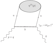
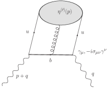
Figure 1: Diagrams corresponding to the leading-order terms in the hard-scattering amplitudes involving the two-particle (left) and three-particle (right) $\eta^{(\prime)}$ DA’s shown by ovals. Solid, curly and wave lines represent quarks, gluons, and external currents, respectively. For $B_{s}\to\eta^{(\prime)}$ transition, $u$ is replaced by $s$. In the case of $D\to\eta^{(\prime)}$ transitions, $u\to d$ and $b\to c$ and correspondingly $d$ is exchanged by $s$ for $D_{s}\to\eta^{(\prime)}$.

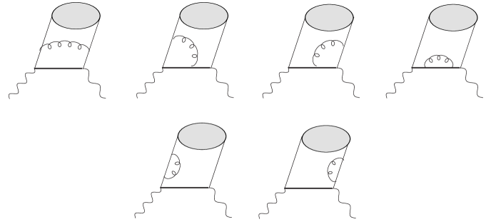
Figure 2: Diagrams contributing to the quark hard-scattering amplitudes at $O(\alpha_{s})$.

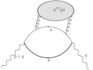
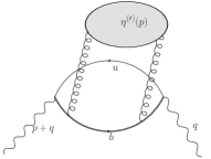
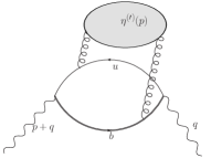
Figure 3: Diagrams contributing to the gluonic hard-scattering amplitudes at $O(\alpha_{s})$.The first diagram is IR divergent and its divergence will be absorbed by the evolution of the gluon DA. See text.

Due to the specific properties of $\eta$ and $\eta^{\prime}$ mesons discussed above, there are additional gluonic diagrams contributing to $M\to\eta^{(\prime)}$ form factors shown in Fig.3. These contribution has only been calculated for $f^{+}_{B\eta^{(\prime)}}$ form factor at twist-2 level in BallJones and for $m^{2}_{\eta^{(\prime)}}=0$. Here we are going to calculate these contributions for other form factors $f^{0}_{M\eta^{(\prime)}}$ and $f^{T}_{M\eta^{(\prime)}}$ by neglecting $O(\alpha_{s}m_{\eta^{(\prime)}})$ effects in both DAs and the hard-scattering part. This approximation is justified having in mind that parameters of DA for the gluonic DA of $\eta$ and $\eta^{\prime}$ are badly known, see the values of $b_{2}^{\eta^{(\prime)},g}$ parameter below.

By using hadronic dispersion relation in the virtuality $(p+q)^{2}$ of the current in the $B$ channel, we can relate the correlation function (55) to the $B\to\eta^{(\prime)}$ matrix elements,

$$\langle\eta^{(\prime)}(p)|\bar{u}\gamma_{\mu}b|\bar{B}(p+q)\rangle=2f^{+}_{B\eta^{(\prime)}}(q^{2})p_{\mu}+\left(f^{+}_{B\eta^{(\prime)}}(q^{2})+f^{-}_{B\eta^{(\prime)}}(q^{2})\right)q_{\mu}\,,$$ (56)

$$\langle\eta^{(\prime)}(p)|\bar{u}\sigma_{\mu\nu}q^{\nu}b|\bar{B}(p+q)\rangle=\Big{[}q^{2}(2p_{\mu}+q_{\mu})-(m_{B}^{2}-m_{\eta^{(\prime)}}^{2})q_{\mu}\Big{]}\frac{if_{B\eta^{(\prime)}}^{T}(q^{2})}{m_{B}+m_{\eta^{(\prime)}}}\,.$$ (57)

and extract the form factors. In the literature it sometimes appears that the form factors are defined as above by divided by a factor $\sqrt{2}$ to match the transition form factors of $\eta,\eta^{\prime}$ with those of a pion when there is no $\eta-\eta^{\prime}$ mixing and in the limit of the conserved SU(3)-flavour symmetry BallJones .

Inserting hadronic states with the $B$-meson quantum numbers between the currents in (55), and isolating the ground-state $B$-meson contributions for all three invariant amplitudes $F(q^{2},(p+q)^{2})$, $\widetilde{F}(q^{2},(p+q)^{2})$ and $F^{T}(q^{2},(p+q)^{2})$ and using (56) and (57) obtains:

$$f^{+}_{B\eta^{(\prime)}}(q^{2})=\frac{e^{m_{B}^{2}/M^{2}}}{2m_{B}^{2}f_{B}}\Bigg{[}F_{0}(q^{2},M^{2},s_{0}^{B})+\frac{\alpha_{s}C_{F}}{4\pi}\left(F_{1}(q^{2},M^{2},s_{0}^{B})+F_{1}^{gg,+}(q^{2},M^{2},s_{0}^{B})\right)\Bigg{]}\,,$$

(58)

$$f^{+}_{B\eta^{(\prime)}}(q^{2})+f^{-}_{B\eta^{(\prime)}}(q^{2})=\frac{e^{m_{B}^{2}/M^{2}}}{m_{B}^{2}f_{B}}\Bigg{[}\widetilde{F}_{0}(q^{2},M^{2},s_{0}^{B})+\frac{\alpha_{s}C_{F}}{4\pi}\widetilde{F}_{1}(q^{2},M^{2},s_{0}^{B})\Bigg{]}\,,$$ (59)

$$f^{T}_{B\eta^{(\prime)}}(q^{2})=\frac{(m_{B}+m_{\eta}^{(\prime)})e^{m_{B}^{2}/M^{2}}}{2m_{B}^{2}f_{B}}\Bigg{[}F^{T}_{0}(q^{2},M^{2},s_{0}^{B})$$

$$\hskip 85.35826pt+\frac{\alpha_{s}C_{F}}{4\pi}\left(F^{T}_{1}(q^{2},M^{2},s_{0}^{B})+F_{1}^{gg,T}(q^{2},M^{2},s_{0}^{B})\right)\Bigg{]}\,.$$ (60)

The scalar $B\to\eta^{(\prime)}$ form factor is then a combination of the vector form factor (58) and the form factor from (59),

$$f^{0}_{B\eta^{(\prime)}}(q^{2})=f^{+}_{B\eta^{(\prime)}}(q^{2})+\frac{q^{2}}{m_{B}^{2}-m_{\eta^{(\prime)}}^{2}}f^{-}(q^{2})$$ (61)

and is only present in the semileptonic $B_{(s)},D_{(s)}\to\eta^{(\prime)}l\nu$ decays when the lepton mass is not neglected and the rare $B_{s},D_{s}\to\eta^{(\prime)}l^{+}l^{-}$ decays. In above, $F_{0(1)}$ and $\widetilde{F}_{0(1)}$ represent the LO (NLO) contributions and $f_{B}=\langle\bar{B}_{d}|m_{b}\bar{b}i\gamma_{5}d|0\rangle/m_{B}^{2}$ is the $B$-meson decay constant. $F_{1}^{gg,(+,T)}$ are leading order twist-2 two-gluon contributions calculated explicitly in the paper. At the leading twist-2 level there is no gluonic contribution in (59). However, note from (61) that this does not mean that twist-2 two-gluon contributions will not appear in the scalar $f^{0}_{M\eta^{(\prime)}}$ form factors (61).

As usual, the quark-hadron duality is used to approximate heavier state contribution by introducing the effective threshold parameter $s_{0}^{B}$ and the ground state contribution of $B$ meson is enhanced by the Borel-transformation in the variable $(p+q)^{2}\to M^{2}$. Completely analogous relations are valid for $B_{s}\to\eta^{(\prime)}$ form factors, with the replacement $u\rightarrow s$ in (56) and (57) and by replacing $m_{B}$ by $m_{B_{s}}$, $f_{B}$ by $f_{B_{s}}$, as well as $M^{2}$ by $M_{s}^{2}$ and $s_{0}^{B}$ by $s_{0}^{B_{s}}$ in (58 - 60). In addition, in the derivation of above expressions for $B_{s}$, one has to take into account that $\langle B_{s}|\bar{b}i\gamma_{5}s|0\rangle/m_{B_{s}}^{2}=f_{B_{s}}/(m_{b}+m_{s})$. The same is valid for $D,D_{s}$ form factors with the replacement $m_{b}\rightarrow m_{c}$ and the appropriate exchanges described before.

The calculation will be performed in $\overline{MS}$ scheme. The $B,B_{s}$ and $D,D_{s}$ decay constants will be calculated in the $\overline{MS}$ scheme using the sum rule expressions from JL with $O(\alpha_{s},m_{s}^{2})$ accuracy. In that way we achieve the consistency of the calculation and the cancellation of uncertainties in the sum rule parameters.

Each form factor can be written in the form of the dispersion relation:

$$F(q^{2},M_{(s)}^{2},s_{0}^{M})=\frac{1}{\pi}\int\limits_{m_{b}^{2}}^{s_{0}^{M}}dse^{-s/M^{2}_{(s)}}\,\mbox{Im}_{s}F(q^{2},s)\,,$$ (62)

where now $s=(p+q)^{2}$.

The leading order parts of the LCSR for $f^{+}_{M\eta^{(\prime)}}$, $f^{+}_{M\eta^{(\prime)}}+f^{-}_{M\eta^{(\prime)}}$ and $f^{T}_{M\eta^{(\prime)}}$ form factors are given in Appendix A.

Up to now, SU(3)-violating effects for $f_{D_{(s)}\eta^{(\prime)}}$, $f_{B_{(s)}\eta^{(\prime)}}$ form factors were not systematically studied, since the effects of inclusion of $m_{\eta^{(\prime)}}^{2}$ effects complicate the calculation, especially at NLO in the hard-scattering amplitudes. However, while the complete SU(3)-symmetry breaking corrections in $\eta^{(\prime)}$ DAs of twist-3 and twist-4 are now known Braun2014 , it is worth to have a consistent picture of all SU(3)-breaking corrections and we will include complete SU(3)-breaking effects in both DAs, as well as in the hard scattering amplitudes at LO. At NLO in the hard-scattering amplitudes, for the cases when the mass of a light quark cannot be neglected, as for $m_{s}$, the inclusion of $m_{s}$ and $m_{\eta^{(\prime)}}^{2}$ effects complicate the calculation. As already known from the analysis of $B_{(s)}\to K$ from factors done in DupliJa , inclusion of quark mass effects leads to the mixing between different twists and the fully consistent calculation with $m_{s}$ included in the quark propagators is not possible, see discussion in DupliJa . However, here we have $\eta^{\prime}$ as a finite-state particle which mass is much larger than $m_{s}$ and therefore, in the NLO quark and gluonic amplitudes we set $m_{s}=0$ and $p^{2}=m_{\eta^{\prime}}^{2}\neq 0$.

Each form factor can be expressed as

$$\left(\begin{matrix}f_{B\eta}^{+,0,T}\\ f_{B\eta^{\prime}}^{+,0,T}\\ \end{matrix}\right)=U(\phi)\left(\begin{matrix}f_{B\eta^{q}}^{+,0,T}\\ f_{B\eta^{s}}^{+,0,T}\\ \end{matrix}\right)\,,$$ (63)

and

$$f_{B\eta^{q}}^{+,0,T}=f_{B\eta^{q}}^{(\bar{q}q)\,+,0,T}+f_{B\eta^{q}}^{(gg)\,+,0,T}\,,\quad f_{B\eta^{s}}^{+,0,T}=f_{B\eta^{s}}^{(gg)\,+,0,T}$$ (64)

and explicitly

$$f_{B\eta}^{+,0,T}=\frac{f_{\eta}^{(q)}}{\sqrt{2}}\left(F_{0}^{\bar{q}q}+F_{1}^{\bar{q}q}\right)+f_{\eta}^{1}F_{1}^{gg,+,0,T}\,,$$

$$f_{B\eta^{\prime}}^{+,0,T}=\frac{f_{\eta^{\prime}}^{(q)}}{\sqrt{2}}\left(F_{0}^{\bar{q}q}+F_{1}^{\bar{q}q}\right)+f_{\eta^{\prime}}^{1}F_{1}^{gg,+,0,T}\,,$$

$$f_{B_{s}\eta}^{+,0,T}=f_{\eta}^{(s)}\left(F_{0}^{\bar{s}s}+F_{1}^{\bar{s}s}\right)+f_{\eta}^{1}F_{1}^{gg,+,0,T}\,,$$

$$f_{B_{s}\eta^{\prime}}^{+,0,T}=f_{\eta^{\prime}}^{(s)}\left(F_{0}^{\bar{s}s}+F_{1}^{\bar{s}s}\right)+f_{\eta^{\prime}}^{1}F_{1}^{gg,+,0,T}\,,$$ (65)

where $F_{0}^{\bar{q}q}$ and $F_{0}^{\bar{s}s}$ ($F_{1}^{\bar{q}q}$ and $F_{1}^{\bar{s}s}$) are LO (NLO) contributions from quark hard-scattering amplitudes for each of the form factors and $F_{1}^{gg}$ is the NLO gluonic contribution proportional to the singlet-flavour decay constants

$$f_{\eta}^{1} = \frac{1}{\sqrt{3}}\left(\sqrt{2}\cos\phi f_{q}-\sin\phi f_{s}\right)\,,$$

$$f_{\eta^{\prime}}^{1} = \frac{1}{\sqrt{3}}\left(\sqrt{2}\sin\phi f_{q}+\cos\phi f_{s}\right)\,.$$ (66)

The $f_{\eta^{(}\prime)}^{(r)}$ decay constants are given in (2.1). Analogous expressions are valid for $D_{(s)}\to\eta^{(\prime)}$ decays.

Obviously, for $B,D\to\eta^{(\prime)}$ transitions the main contribution comes from $\eta_{q}$ meson states and $\eta_{s}$ contributes only through suppressed gluonic contributions, while for $B_{s},D_{s}\to\eta^{(\prime)}$ transitions the leading $\eta_{s}$ meson state contribution will receive, through the gluonic diagrams, a small mixture with $\eta_{q}$ state. Also, implicitly there will be mixing with among twist-2 quark and gluonic distribution amplitudes Eq.(32), which will bring $b_{2}^{\eta^{(\prime),g}}$ dependence in the twist-2 quark LO ($F_{0}^{\bar{q}q}$ and $F_{0}^{\bar{s}s}$ ) and NLO contributions ($F_{1}^{\bar{q}q}$ and $F_{1}^{\bar{s}s}$) and $a_{2}^{\eta^{(\prime),1}}$ dependence to the gluonic contributions $F_{1}^{gg}$.

Since $\eta$ and $\eta^{\prime}$ are mixtures of the $|\bar{q}q\rangle$, $|\bar{s}s\rangle$ in the calculation of the quark contributions we will use (with appropriate substitutions) our NLO results for the hard-scattering part for $B\to\pi$ DKMMO and $B_{(s)}\to K$ form factors DupliJa with the $p^{2}$ effects included at the LO (up to twist-4) and NLO level (up to twist-3) and will imply recently derived DAs of $\eta$ and $\eta^{\prime}$ with the SU(3)-breaking effects and the axial anomaly contributions included up to twist-4. The gluonic contributions, which are already NLO effect, will be calculated for $p^{2}=m_{\eta^{(\prime)}}^{2}=0$.

4 LCSR for gluonic contributions to the form factors and consistent treatment of the IR divergences appearing

The gluonic contributions at the $O(\alpha_{s})$ to the $B(D)\to\eta^{(\prime)}$ and $B_{s}(D_{s})\to\eta^{(\prime)}$ form factors come from the diagrams in Fig.3. The results for the form factors $f_{M\eta^{(\prime)}}^{+,0,T}$ are presented in subsection 4.1. They are added to the quark contributions (65) to get the complete result at the order $O(\alpha_{s})$.

The first diagram is Fig.3 is IR (collinear) divergent. This divergence has to disappear for the general collinear factorization formula used here

$$F(q^{2},(p+q)^{2})=\sum_{n}T_{H}^{(n)}(u,q^{2},(p+q)^{2},\mu_{F})\,\otimes\,\Phi_{n,P}(u,\mu_{F})\,,\quad\otimes=\int_{0}^{1}du\,.$$ (67)

be valid. The scale $\mu_{F}$ is the factorization scale. At the twist $n=2$ level, as already mentioned, there will be mixing of quark and gluonic contributions and the hard-scattering (perturbative part) $T_{H}^{(2)}$ and the distribution amplitude $\Phi_{2}$ can be represented as

$$T_{H}^{(2)}=\left(\begin{matrix}T_{q\bar{q}}\\ T_{gg}\end{matrix}\right)\,,\quad\Phi_{2,P}=\left(\begin{matrix}\phi_{2,P}^{q}\\ \phi_{2,P}^{q}\end{matrix}\right)\,.$$ (68)

In order to consistently treat this mixing we have to examine the evolution of the DAs, at the same $O(\alpha_{s})$ as the calculation of the perturbative part $T_{H}$. Due to the mixing the standard Brodsky-Lepage (BL) evolution equation ERBL

$$\mu_{F}\frac{\partial}{\partial\mu_{F}}\psi(u,\mu_{F})=V(u,v,\mu_{F})\,\otimes\,\psi(v,\mu_{F})\,,$$ (69)

will be a matrix equation now, where $V(u,v,\mu_{F})$ is the perturbatively calculable evolution kernel

$$V(u,v,\mu_{F}) = \frac{\alpha_{S}(\mu_{F})}{4\pi}\,V_{1}(u,v)+\frac{\alpha_{S}^{2}(\mu_{F})}{(4\pi)^{2}}V_{2}(u,v)+\cdots\,,$$ (70)

with the LO kernel of our interest of the form

$$V_{1}(u,v) = \left(\begin{matrix}V_{qq}&&V_{qg}\\ V_{gq}&&V_{gg}\end{matrix}\right)$$ (71)

and $V_{ij}$ are well-know evolution kernels Terentev ; baier ; KrollPassek which we cite here for convenience:

$$V_{qq}(u,v) = 2C_{F}\left\{\frac{u}{v}\left[1+\frac{1}{v-u}\right]\Theta(v-u)+\left(\begin{matrix}u\to 1-u\\ v\to 1-v\end{matrix}\right)\right\}_{+}\,,$$

$$V_{qg}(u,v) = -2\sqrt{n_{f}C_{F}}\left\{\frac{u}{v^{2}}\Theta(v-u)-\left(\begin{matrix}u\to 1-u\\ v\to 1-v\end{matrix}\right)\right\}\,,$$

$$V_{gq}(u,v) = 2\sqrt{n_{f}C_{F}}\left\{\frac{u^{2}}{v}\Theta(v-u)-\left(\begin{matrix}u\to 1-u\\ v\to 1-v\end{matrix}\right)\right\}\,,$$

$$V_{gg}(u,v) = 2N_{c}\left\{\frac{u}{v}\left[\left(\frac{\Theta(v-u)}{v-u}\right)_{+}+\frac{2u-1}{v}\Theta(v-u)\right]+\left(\begin{matrix}u\to 1-u\\ v\to 1-v\end{matrix}\right)\right\}+\beta_{0}\delta(u-v)\,.$$

These evolution kernels are exactly those which govern the renormalization of the DAs

$$\Phi(u)=Z_{\phi,ren}(u,v,\mu_{R}^{2})\,\otimes\,\Phi(v,\mu_{R}^{2})\,.$$ (73)

The connection between $Z$ and the evolution kernel $V$ is given as

$$V({\mu}_{R}^{2})=-Z_{\phi,ren}^{-1}({\mu}_{R}^{2})\,\left({\mu}_{R}^{2}\frac{\partial}{\partial{\mu}_{R}^{2}}Z_{\phi,ren}({\mu}_{R}^{2})\right)\,,\\ Z_{\phi,ren}({\mu}_{R}^{2})=1+\frac{\alpha_{S}(\mu_{R})}{4\pi}\,\frac{1}{\epsilon}V_{1}(u,v)+\cdots\,.$$

($D=4-2\epsilon$). On the other hand, by calculating the hard-scattering part $T_{H}$, owing to the fact that final-state quarks are taken to be massless and on-shell (for the case $p^{2}=0$), the amplitude contains collinear singularities. Since $T_{H}$ is a finite quantity by definition, collinear singularities have to be subtracted. Therefore, $T$ factorizes as

$$T(u,Q^{2})=T_{H}(v,Q^{2},\mu_{F})\,\otimes\,Z_{T,col}(v,u;\mu_{F})\,,$$ (74)

with collinear singularities being subtracted at the scale $\mu_{F}$ and absorbed into the constant $Z_{T,col}$. As usual The UV singularities are removed by the renormalization of the fields and by the coupling-constant renormalization at the (renormalization) scale $\mu_{R}$. Now, in order that the factorization formula is valid, the following has to be satisfied

$$Z_{T,col}(u,v;\mu_{F})\otimes Z_{\phi,ren}(v,\omega;\mu_{F})=\delta(v-\omega)\,.$$ (75)

The divergences of $T(u,Q^{2})$ and $\Phi(u)$ in (67) then cancel and at the end we are left with the finite perturbative expressions for all form transition factors

$$F(q^{2},(p+q)^{2})=T_{H}(u,Q^{2},\mu_{F})\,\otimes\,\Phi(u,\mu_{F})\,.$$ (76)

It is worth pointing out that the scale $\mu_{F}$ representing the boundary between the low- and high-energy parts in (67) plays the role of the separation scale for collinear singularities in $T(u,Q^{2})$, on the one hand, and of the renormalization scale for UV singularities appearing in the perturbatively calculable part of the distribution amplitude $\Phi(u)$, on the other hand. The general discussion and all details of the proof of the cancellation of the factorization scale dependence in the collinear factorization formula (67) at all orders of calculation can be found in MelicMALI ; NizicMI .

In our case of calculating the heavy-to-light transition form factors $f^{+,0,T}$ we face the following situation. The hard-scattering, perturbatively calculable pieces coming from the diagrams from Fig.2 have UV and infra-red singularities at $O(\alpha_{s})$. We have already proven in RucklK ; DKMMO ; DupliJa for $B\to\pi$ and $B_{(s)}\to K$ form factors that the IR divergences of the quark contributions at twist 2 level cancel exactly with those coming from the evolution kernel $V_{qq}$. Here, due to the mixing with the twist 2 gluonic contributions, the convolution of $V_{qg}$ of the $T_{H}$ LO will exactly cancel the IR divergence in the first gluonic diagram in Fig.3. At the twist 3 level of $O(\alpha_{s})$ the IR divergences of quark diagrams mutually cancel, as shown before in DKMMO ; DupliJa . This gives the final proof of the collinear factorization formula at the given order for the heavy-to-light $M\to\eta^{\prime}$ transition form factors.

4.1 Explicit results for the leading two-gluon contributions to the $f^{+}$ and $f^{T}$ form factors in $B,B_{s}\to\eta^{(\prime)}$ and $D,D_{s}\to\eta^{(\prime)}$ transitions

In the calculation of the gluonic contributions to the form factors we have faced the problem of the consistent treatment of the $\gamma_{5}$ in the dimensional regularization. Leading order for the gluonic amplitude is given by one-loop Feynman diagrams in Fig.3. and we have to deal with IR divergence which is a consequence of having massless quarks propagating through the loops. In the calculation of the gluonic contributions to the form factors it appears a Levi-Civita tensor in the projector of the twist-2 two-gluon DA (31) and a single $\gamma_{5}$ matrix in the trace which are both quantities with well-defined properties only in $D=4$ space-time dimensions. Generalization of these quantities in $D$ dimensions is problematic and different approaches to avoid resulting ambiguities can be found in the literature. Moreover, in our case there is no gluonic contributions which appear at LO on $\alpha_{s}$ that would greatly help in resolving the $\gamma_{5}$ problem at NLO level. The problem was not addressed in the paper where the gluonic amplitude was evaluated for the first time BallJones and it is not clear how they resolved the ambiguities.

In the case of the interest it is possible to completely avoid $\gamma_{5}$ problem and all connected complications since the IR divergence is direct consequence of the massless quark lines and putting a small mass $m$ in massless quark propagators regularizes (removes) the divergence. As a consequence, we are not forced to use dimensional regularization and calculation can be performed in four dimensions without any problem. Note that putting mass in quark propagators doesn’t spoil any of properties and symmetries of the amplitude contrary to the case when, so called, mass regularization is used on gluon propagators. At the very end of calculation it is necessary to expand final result around zero for the small introduced quark mass $m$. The IR divergence will now reappear as $\ln(m^{2})$ term and it is straightforward to connect it with 1/($D$-4) term in the framework of dimensional regularization.

The obtained expressions are as follows:

$$F_{1}^{gg,i}(q^{2},M^{2},s_{0}^{M})=f_{\eta^{(\prime)}}^{1}b_{2}^{\eta^{(}\prime),g}\frac{1}{C_{F}}\int_{m^{2}}^{s_{0}^{M}}\exp^{-s/M^{2}}f^{gg,i}(s,q^{2})\,,$$ (77)

where the gluonic contribution to $f^{+}$ form factors is

$$f^{gg,+} = 20m^{2}\frac{(s-m^{2})}{27\sqrt{3}(s-q^{2})^{5}}\bigg{(}3(m^{2}-q^{2})(5m^{4}-5m^{2}(q^{2}+s)+q^{4}+3q^{2}s+s^{2})$$

$$\left.\left(2\ln\left(\frac{s-m^{2}}{m^{2}}\right)-\ln\left(\frac{\mu^{2}}{m^{2}}\right)\right)\right.$$

$$-\left(37m^{6}-m^{4}\left(56q^{2}+55s\right)+m^{2}\left(18q^{4}+76q^{2}s+17s^{2}\right)+3q^{6}-27q^{4}s-11q^{2}s^{2}-2s^{3}\right)\bigg{)}$$

and the corresponding contribution to $f^{T}$ form factors has the following form

$$f^{gg,T}=5m\frac{s-m^{2}}{27\sqrt{3}(s-q^{2})^{5}}\bigg{(}12q^{2}\frac{s}{s-m^{2}}\left(q^{4}+3q^{2}s+s^{2}\right)\ln\left(\frac{s}{m^{2}}\right)$$

$$\left.+6(m^{2}-q^{2})\left(5m^{4}-5m^{2}(q^{2}+s)+q^{4}+3q^{2}s+s^{2}\right)\left(2\ln\left(\frac{s-m^{2}}{m^{2}}\right)-\ln\left(\frac{\mu^{2}}{m^{2}}\right)\right)\right.$$

$$-\left(59m^{6}-m^{4}(72q^{2}+85s)+m^{2}s(84q^{2}+23s)+3(6q^{6}+6q^{4}s+6q^{2}s^{2}-s^{3})\right)\bigg{)}$$

(79)

with $m=m_{c,b}$.

With respect to the fact there is no LO $O(\alpha_{s}^{0})$ twist-2 gluon contributions and following the discussions at the beginning of Sec.4, obviously there is no gluonic contributions to $f^{+}+f^{-}$ form factors at this order of calculation.

The result for the gluonic $O(\alpha_{s})$ contribution to $f^{+}$ form factors was first given in the appendix of BallJones . Our result (LABEL:eq:fplusg) does not completely agree with the one presented there. While we agree in the part being proportional to the logarithmic terms, there is a disagreement between the coefficients in the second line of (LABEL:eq:fplusg) and the expression (A.1) from BallJones . Since those terms are exactly those which change with the different treatment of $\gamma_{5}$, and the authors of BallJones have not placed any comment how they have resolved the $\gamma_{5}$ ambiguities in the calculation of $f^{gg,+}$, we assume that the difference comes from the improper treatment of the $\gamma_{5}$ in BallJones .

The result for the gluonic $O(\alpha_{s})$ contribution to $f^{T}$, Eq.(79) is a new result.

5 Predictions for $B,B_{s}\to\eta^{(\prime)}$ and $D,D_{s}\to\eta^{(\prime)}$ form factors ($f^{+},f^{0}$ and $f^{T}$) the form factors

The prediction for $B,B_{s}\to\eta^{(\prime)}$ and $D,D_{s}\to\eta^{(\prime)}$ form factors ($f^{+},f^{0}$ and $f^{T}$) the form factors will be given in the $\overline{MS}$ scheme by using the input parameters listed in Appendix B.

From expressions (59,60,61) we see that we need the heavy-meson decay constants of $B_{(s)}$ and $D_{(s)}$ in the calculation. As usually done, to achieve partial cancellation of the uncertainties in the calculation the two-point QCD sum rules for the decay constants $f_{B},f_{B_{s}}$ and $f_{D},f_{D_{s}}$ is used in the same scheme, with $O(\alpha_{s},m_{s}^{2})$ corrections included JL . We have used the same level of accuracy as in the calculation of the form factors, i.e ${\cal O}(\alpha_{s})$ in both, the perturbative and nonperturbative (quark condensate) part and in the determination of the sum rules parameters $\overline{s}_{0}^{B_{(s)}}$ and $\overline{M}_{(s)}^{2}$ have used the usual consistency conditions in the sum rule calculations.

The resulting predictions for $f_{M}$, together with the fitted sum rule parameters for each of the mesons are given in the Appendix B, Tables 2-4. Here we quote the calculated values from Table 4:

$$f_{D}=191\pm 9\;{\rm MeV},\,f_{D_{s}}=219\pm 7\;{\rm MeV}\,,$$

$$f_{B}=215\pm 7\;{\rm MeV},\,f_{B_{s}}=246\pm 8\;{\rm MeV}\,,$$ (80)

where the quoted error intervals are coming from the variation of $\overline{s}_{0}^{M}$ and $\overline{M}_{M}^{2}$ only since other uncertainties are canceled in ratios in Eqs.(59,60,61). By comparing our results with the previous LCSR results and the most recent determinations from KhodjamPivovarov , where in the perturbative part the higher order corrections were included, we see good agreement. The results are also within uncertainties of the lattice QCD calculations of the same decay constants latticeDC .

For the $f_{D}$ and $f_{D_{s}}$ the experiment gives somewhat larger values PDG2014 ,

$$f_{D}=204.6\pm 5.0\;{\rm MeV},\,f_{D_{s}}=257.5\pm 4.6\;{\rm MeV}\,,$$

but still consistent within the complete LCSR error results KhodjamPivovarov .

The renormalization scale is given by the expression $\mu_{B_{(}s)}=\sqrt{m_{B_{(s)}}^{2}-m_{b}^{2}}$ and similarly for $D_{(s)}\to\eta^{(\prime)}$ transitions. Therefore, for the renormalization scale we use $\mu=3$ GeV, for the $f_{B\eta^{(\prime)}}^{0,+,T}$ form factors and $\mu_{s}=3.4$ GeV for $f_{B_{s}\eta^{(\prime)}}^{0,+,T}$ and for $\mu_{D}=1.4$ GeV and $\mu_{D_{s}}=1.5$ GeV. As usual, we will check the sensitivity of the results on the variation of above scales and will include it in the error estimation.

The method of extraction of the Borel parameters $M$ and the effective thresholds $s_{0}$ for $f_{M\eta^{(\prime)}}^{+,0,T}$ form factors is the same as described in DKMMO . It relies on the requirement that the derivative over $-1/M^{2}$ of the expression of the complete LCSR for a particular form factor, which gives heavy-meson masses $m_{M}^{2}$, does not deviate more than $0.5-2.5\%$ from the experimental values for those masses. Additional requirements such as that the subleading twist-4 terms in the LO, are small, less than $10\%$ of the LO twist-2 term, that the NLO corrections of twist-2 and twist-3 parts are not exceeding $30\%$ of their LO counterparts, and that the subtracted continuum remains small, are also satisfied. These demands provide us the central values for the LCSR parameters listed in Tab.5.

The estimated form factors for $B_{(s)}\to\eta^{(\prime)}$ are as follows:

$$f^{+}_{B\eta}(0) = 0.168^{+0.041}_{-0.047}=0.168\pm 0.003\,(b_{2}^{\eta,g})\pm 0.002(s_{0},M)\pm^{0.041}_{0.047}({\rm mix})\pm^{0.005}_{0.003}({\rm rest})\,,$$

$$f^{+}_{B\eta^{\prime}}(0) = 0.130^{+0.036}_{-0.032}=0.130\pm 0.020\,(b_{2}^{\eta^{\prime},g})\pm 0.002(s_{0},M)\pm^{0.030}_{0.032}({\rm mix})\pm^{0.005}_{0.002}({\rm rest})\,,$$

$$|f^{+}_{B_{s}\eta}(0)| = 0.212^{+0.015}_{-0.013}=0.212\pm 0.003\,(b_{2}^{\eta,g})\pm 0.003(s_{0},M)\pm 0.012({\rm mix})\pm^{0.008}_{0.003}({\rm rest})\,,$$

$$f^{+}_{B_{s}\eta^{\prime}}(0) = 0.252^{+0.023}_{-0.020}=0.252\pm 0.019\,(b_{2}^{\eta^{\prime},g})\pm 0.004(s_{0},M)\pm 0.005({\rm mix})\pm^{0.011}_{0.002}({\rm rest})\,,$$

$$f^{T}_{B\eta}(0) = 0.173^{+0.041}_{-0.035}=0.173\pm 0.002\,(b_{2}^{\eta,g})\pm 0.003(s_{0},M)\pm^{0.040}_{0.035}({\rm mix})\pm^{0.007}_{0.003}({\rm rest})\,,$$

$$f^{T}_{B\eta^{\prime}}(0) = 0.141^{+0.032}_{-0.030}=0.141\pm 0.015\,(b_{2}^{\eta^{\prime},g})\pm 0.002(s_{0},M)\pm^{0.028}_{0.026}({\rm mix})\pm^{0.006}_{0.003}({\rm rest})\,,$$

$$|f^{T}_{B_{s}\eta}(0)| = 0.225^{+0.019}_{-0.014}=0.225\pm 0.002\,(b_{2}^{\eta,g})\pm 0.004(s_{0},M)\pm^{0.014}_{0.013}({\rm mix})\pm^{0.012}_{0.002}({\rm rest})\,,$$

$$f^{T}_{B_{s}\eta^{\prime}}(0) = 0.280^{+0.022}_{-0.016}=0.280\pm 0.014\,(b_{2}^{\eta^{\prime},g})\pm 0.004(s_{0},M)\pm^{0.006}_{0.007}({\rm mix})\pm^{0.015}_{0.002}({\rm rest})\,,$$

and for $D_{(s)}\to\eta^{(\prime)}$:

$$f^{+}_{D\eta}(0) = 0.429^{+0.165}_{-0.141}=0.429\pm 0.009\,(b_{2}^{\eta,g})\pm^{0.004}_{0.001}(s_{0},M)\pm^{0.164}_{0.141}({\rm mix})\pm^{0.013}_{0.008}({\rm rest})\,,$$

$$f^{+}_{D\eta^{\prime}}(0) = 0.292^{+0.113}_{-0.104}=0.292\pm 0.045\,(b_{2}^{\eta^{\prime},g})\pm^{0.009}_{0.007}(s_{0},M)\pm^{0.099}_{0.091}({\rm mix})\pm^{0.015}_{0.011}({\rm rest})\,,$$

$$|f^{+}_{D_{s}\eta}(0)| = 0.495^{+0.030}_{-0.029}=0.495\pm 0.007\,(b_{2}^{\eta,g})\pm^{0.004}_{0.002}(s_{0},M)\pm^{0.027}_{0.024}({\rm mix})\pm^{0.016}_{0.009}({\rm rest})\,,$$

$$f^{+}_{D_{s}\eta^{\prime}}(0) = 0.557^{+0.048}_{-0.045}=0.557\pm 0.041\,(b_{2}^{\eta^{\prime},g})\pm^{0.011}_{0.008}(s_{0},M)\pm^{0.010}_{0.008}({\rm mix})\pm^{0.022}_{0.014}({\rm rest})\,,$$

$$f^{T}_{D\eta}(0) = 0.435^{+0.115}_{-0.107}=0.435\pm 0.008\,(b_{2}^{\eta,g})\pm^{0.005}_{0.003}(s_{0},M)\pm^{0.112}_{0.106}({\rm mix})\pm^{0.177}_{0.151}({\rm rest})\,,$$

$$f^{T}_{D\eta^{\prime}}(0) = 0.337^{+0.118}_{-0.147}=0.337\pm 0.055\,(b_{2}^{\eta^{\prime},g})\pm^{0.013}_{0.051}(s_{0},M)\pm^{0.100}_{0.101}({\rm mix})\pm^{0.080}_{0.077}({\rm rest})\,,$$

$$|f^{T}_{D_{s}\eta}(0)| = 0.441^{+0.091}_{-0.087}=0.441\pm 0.007\,(b_{2}^{\eta,g})\pm^{0.052}_{0.005}(s_{0},M)\pm^{0.030}_{0.031}({\rm mix})\pm^{0.068}_{0.082}({\rm rest})\,,$$

$$f^{T}_{D_{s}\eta^{\prime}}(0) = 0.655^{+0.072}_{-0.065}=0.655\pm 0.050\,(b_{2}^{\eta^{\prime},g})\pm^{0.015}_{0.014}(s_{0},M)\pm^{0.036}_{0.030}({\rm mix})\pm^{0.034}_{0.026}({\rm rest})\,.$$

These results are predictions given with $b_{2}^{\eta^{(\prime),g}}=0$ and then varied within the interval $\Delta b_{2}^{\eta^{(\prime),g}}=\pm 20$, which dependence is explicitly displayed in the errors. The errors are compilation of the variation of parameters added in quadratures. In the errors we explicitly stress SR parameter dependence $(s_{0},\,M)$, $\eta-\eta^{\prime}$ mixing parameter dependence (mix) and dependences coming from the variation of the rest of parameters (rest=$\{\mu,\,m_{c,b},\,a_{2},\,a_{4}\}$).

The errors of the results are much larger for the transitions $B,D\to\eta^{(\prime)}$ where $B,D\to\eta_{q}$ dominates then for $B_{s},D_{s}\to\eta_{s}$ decays since the error in the parameter $h_{q}$ (37) is huge, of $O(200\%)$ depending not on $\eta-\eta^{\prime}$ mixing parameters but exhibiting a numerical cancellation among terms. If one would use approximation (35) applied in Offen instead, the (rest)-errors would be almost an order of magnitude lower and the mean values would be somewhat larger for those decays, which we assume is the main reason, apart from the rest of $SU(3)_{F}$ approximations used there, of the discrepancies with some of the results presented in Offen . We see that the dominant errors in $M\to\eta^{\prime}$ form factors is coming from the variation of $b_{2}^{\eta^{(\prime),g}}$ and it amounts to about $15\%$, while in $M\to\eta$ decays come to $2\%$. Our findings for calculated $B\to\eta^{(\prime)}$ form factors agree very well with those from BallJones ; Li ; Aliev1 ; Aliev2 .

Their $q$-dependence of the form factors and their ratios is shown in Fig.4-9.

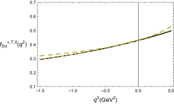
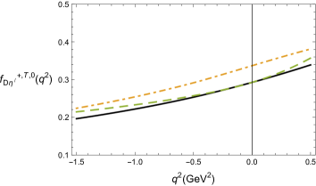
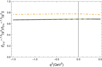
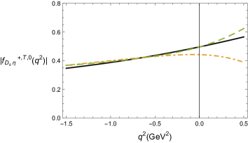
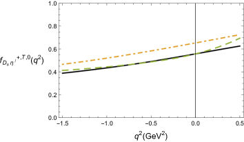
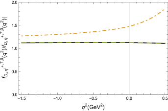
Figure 4: Form factors for $D_{(s)}\to\eta^{(\prime)}$ decays and their ratios. Solid lines represent $f_{D_{(s)}\eta^{(\prime)}}^{+}$ form factors, dashed-dotted line $f_{D_{(s)}\eta^{(\prime)}}^{T}$ and dashed line $f_{D_{(s)}\eta^{(\prime)}}^{0}$ form factors.

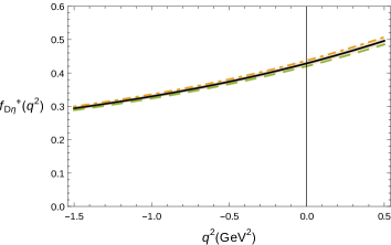
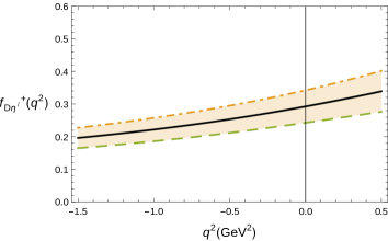
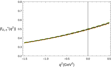
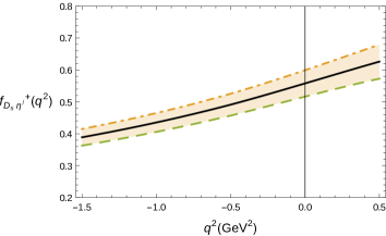
Figure 5: Gluonic dependence of $f_{D_{(s)}\eta^{(\prime)}}^{+}$ form factors. Shaded areas show change of the form factors under the variation of $b_{2}^{\eta^{(\prime)},g}=0\pm 20$. Solid line denotes the result for $b_{2}^{\eta^{(\prime)},g}=0$, dashed-dotted for $b_{2}^{\eta^{(\prime)},g}=20$ and dashed line for $b_{2}^{\eta^{(\prime)},g}=-20$.

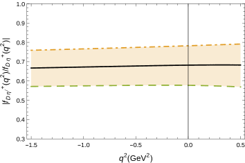
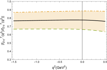
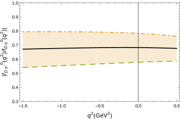
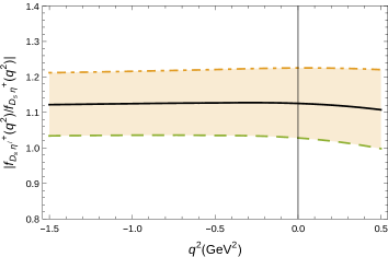
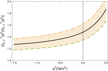
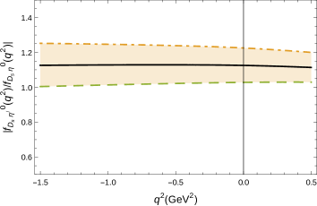
Figure 6: Gluonic dependence of ratios of $D_{(s)}\to\eta^{(\prime)}$ form factor ratios. Shaded areas show change of the form factors under the variation of $b_{2}^{\eta^{(\prime)},g}=0\pm 20$. Solid line denotes the result for $b_{2}^{\eta^{(\prime)},g}=0$, dashed-dotted for $b_{2}^{\eta^{(\prime)},g}=20$ and dashed line for $b_{2}^{\eta^{(\prime)},g}=-20$.

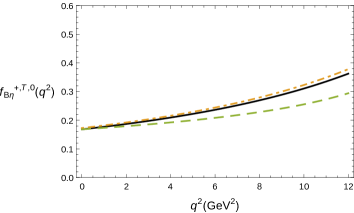
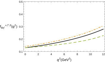
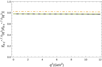
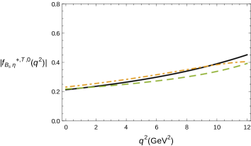
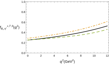
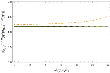
Figure 7: Form factors for $B_{(s)}\to\eta^{(\prime)}$ decays and their ratios. Solid lines represent $f_{B_{(s)}\eta^{(\prime)}}^{+}$ form factors, dashed-dotted line $f_{B_{(s)}\eta^{(\prime)}}^{T}$ and dashed line $f_{B{(s)}\eta^{(\prime)}}^{0}$ form factors.

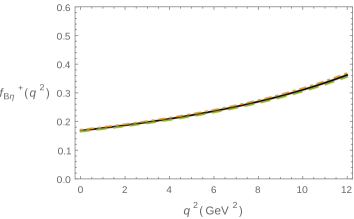
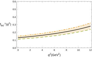
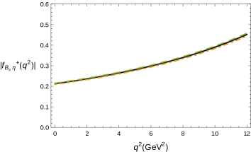
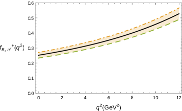
Figure 8: Gluonic dependence of $f_{B_{(s)}\eta^{(\prime)}}^{+}$ form factors. Shaded areas show change of the form factors under the variation of $b_{2}^{\eta^{(\prime)},g}=0\pm 20$. Solid line denotes the result for $b_{2}^{\eta^{(\prime)},g}=0$, dashed-dotted for $b_{2}^{\eta^{(\prime)},g}=20$ and dashed line for $b_{2}^{\eta^{(\prime)},g}=-20$.

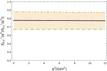
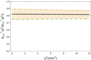
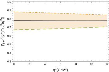
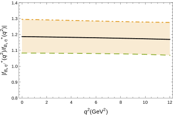
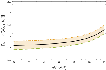
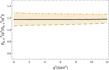
Figure 9: Gluonic dependence of ratios of $B_{(s)}\to\eta^{(\prime)}$ form factor ratios. Shaded areas show change of the form factors under the variation of $b_{2}^{\eta^{(\prime)},g}=0\pm 20$. Solid line denotes the result for $b_{2}^{\eta^{(\prime)},g}=0$, dashed-dotted for $b_{2}^{\eta^{(\prime)},g}=20$ and dashed line for $b_{2}^{\eta^{(\prime)},g}=-20$.

From Fig.5 and Fig.8 we see that the gluonic corrections are much larger for $B_{(s)},D_{(s)}\to\eta^{\prime}$ decays then for $M\to\eta$, as expected. Also the gluonic corrections are larger in $D_{(s)}$ decays. It is obvious that even in ratios of form factors the gluonic contributions give main error and that it would be difficult to constrain $b_{2}$, unless all $M\to\eta^{(\prime)}$ semileptonic transitions are measured, Fig. 6 and 9.

We can now investigate $\rm{SU(3)_{F}}$ approximations from (17). By using the obtained results and the result for $f_{BK}$ from DupliJa we obtain

$$|f_{B_{s}\eta}^{+}|^{\rm calc}=0.212^{+0.015}_{-0.013}\quad{\rm vs}\quad|f_{B_{s}\eta}^{+,\rm approx}|=0.225^{+0.032}_{-0.026}\,,$$

$$f_{B_{s}\eta^{\prime}}^{+,\rm calc}=0.252^{+0.023}_{-0.020}\quad{\rm vs}\quad|f_{B_{s}\eta^{\prime}}^{+,\rm approx}|=0.278^{+0.038}_{-0.031}\,.$$

We can note that the approximation works quite well although somewhat better for $M\to\eta$ decays than for $M\to\eta^{\prime}$ transitions.

There exists LCSR calculations of $f_{D_{s}\eta}^{+}$ form factor ColangeloFazio ; Azizi . In these papers the $f_{D_{s}\eta^{\prime}}^{+}$ form factor is then obtained by using the relation

$$\frac{f_{D_{s}\eta^{\prime}}^{+}}{f_{D_{s}\eta}^{+}}=\cot\phi\,.$$ (86)

While their predictions for $f_{D_{s}\eta}^{+}$ agree with ours, the use of the above approximative relation which neglects the gluonic contributions gives somewhat larger $f_{D_{s}\eta^{\prime}}^{+}$ form factor then the one obtained here, (LABEL:eq:results52,LABEL:eq:results54).

There exist also recent lattice results on $D_{s}\to\eta^{(\prime)}$ form factors Bali . These transitions at the lattice are challenging due to the presence of disconnected quark-line contributions and in Bali only the scalar $f_{D_{s}\eta^{(\prime)}}^{0}$ form factors are calculated, which at $q^{2}=0$ are equal to the $f^{+}$. By comparing the results one can see that the lattice predictions give $f_{D_{s}\eta^{\prime}}^{+}<f_{D_{s}\eta}^{+}$, which is just opposite in LCSR for all $M_{s}\to\eta^{(\prime)}$ transitions. The tendency $f_{M\eta^{\prime}}^{+}<f_{M\eta}^{+}$ in LCSR is established for non-strange meson decays, see results in (LABEL:eq:results52,LABEL:eq:results54).

6 Phenomenological applications

In this section we comment on some phenomenological results for semileptonic $D_{(s)}\to\eta^{(\prime)}$ and $B_{(s)}\to\eta^{(\prime)}$ decays which include the calculated from factors. To be able to calculate the branching ratio we need the form factor extracted in whole accessible kinematical regions. For $D_{(s)}$ decays the LCSR are applicable only in the region $q^{2}\ll m_{c}^{2}$ and for $B_{(s)}$ the region is $0<q^{2}<12$ GeV.

The are many parametrization for calculating the shape of form factors at $q^{2}\neq 0$. All of them work equally well and therefore we decided to use the most simplest one BK :

$$f^{{+,T}}_{M\eta^{(\prime)}}(q^{2})_{|{\rm fit}} = f^{(+,T)}_{M\eta^{(\prime)}}(0)\frac{1}{(1-q^{2}/m_{H^{\ast}}^{2})(1-\alpha^{+,T}\,q^{2}/m_{H^{\ast}}^{2})}$$

$$f^{{0}}_{M\eta^{(\prime)}}(q^{2})_{|{\rm fit}} = f^{0}_{M\eta^{(\prime)}}(0)\frac{1}{(1-\alpha^{0}\,q^{2}/m_{H^{\ast}}^{2})}$$ (87)

where the extrapolation of the form factors is performed just by fitting one parameter $\alpha^{i}$ for each of the decays and using the appropriate vector meson resonances $m_{H}^{\ast}$, Tab.6, while the normalization is given by the form factors at $q^{2}=0$. The fitted parameters $\alpha^{i}$ for $D_{(s)}$ form factors are

$$\alpha^{+}_{D\eta} = 0.17\pm 0.07\,,\quad\alpha^{+}_{D\eta^{\prime}}=0.20\pm 0.20$$

$$\alpha^{+}_{D_{s}\eta} = 0.20\pm 0.01\,,\quad\alpha^{+}_{D_{s}\eta^{\prime}}=0.20\pm 0.04$$ (88)

while for $B_{(s)}$ are as follows:

$$\alpha^{+}_{B\eta} = 0.46\pm 0.06\,,\quad\alpha^{0}_{B\eta}=1.00\pm 0.28\,,\quad\alpha^{T}_{B\eta}=0.49\pm 0.05$$

$$\alpha^{+}_{B\eta^{\prime}} = 0.45\pm 0.17\,,\quad\alpha^{0}_{B\eta^{\prime}}=1.00\pm 0.35\,,\quad\alpha^{T}_{B\eta^{\prime}}=0.48\pm 0.11$$

$$\alpha^{+}_{B_{s}\eta} = 0.51\pm 0.02\,,\quad\alpha^{0}_{B_{s}\eta}=1.08\pm 0.06\,,\quad\alpha^{T}_{B_{s}\eta}=0.19\pm 0.11$$

$$\alpha^{+}_{B_{s}\eta^{\prime}} = 0.49\pm 0.03\,,\quad\alpha^{0}_{B_{s}\eta^{\prime}}=1.09\pm 0.11\,,\quad\alpha^{T}_{B_{s}\eta^{\prime}}=0.52\pm 0.04\,.$$ (89)

The large uncertinties of the $\alpha$ parameters are predominantly coming from the large uncertinties in the $\eta-\eta^{\prime}$ mixing parameters.

The semileptonic $D_{(s)}\to\eta^{(\prime)}e\nu_{e}$ and $B\to\eta^{(\prime)}e\nu_{e}$ decay rates are calculated by

$$\Gamma(H\to\eta^{(\prime)}l\bar{\nu_{l}})=\frac{G_{F}^{2}|V_{Qq}|^{2}}{192\pi^{3}m_{H}^{3}}\int_{m_{l}^{2}}^{(m_{H}-m_{\eta^{(\prime)}})^{2}}dq^{2}\lambda^{3/2}(q^{2})|f^{+}_{H\eta^{(\prime)}}(q^{2})|^{2}\,,$$ (90)

where $H=D,D_{s},B$ and $\lambda(q^{2})=(m_{H}^{2}+m_{\eta^{(\prime)}}^{2}-q^{2})^{2}-4m_{H}^{2}m_{\eta^{(\prime)}}^{2}$ and $V_{Qq}=V_{cd},V_{cs},V_{ub}$ depending if $D^{+},D_{s}^{+}$ or $B^{+}$ meson is decaying, respectively. Values for the CKM matrix elements are taken from PDG2014 : $V_{cd}=0.225,V_{cs}=0.973,V_{ub}=0.0035,V_{ts}=0.0405,V_{tb}=0.999.$ (for $V_{ub}$ we used newly determined average value also from PDG2014 ).

For the rare $B_{s}\to\eta^{(\prime)}l^{+}l^{-}(\nu\bar{\nu})$ decays we use the effective Standard Model hamiltonian for $b\to sl^{+}l^{-}(\nu\bar{\nu})$ transitions Buchalla and calculate decay rates as DeFazio1

$$\Gamma(B_{s}\to\eta^{(\prime)}l^{+}l^{-})=\frac{G_{F}^{2}|V_{tb}V_{ts}^{\ast}|^{2}\alpha^{2}}{512\pi^{5}m_{B_{s}}^{3}}\int_{4m_{l}^{2}}^{(m_{B_{s}}-m_{\eta^{(\prime)}})^{2}}dq^{2}\lambda^{1/2}(q^{2})\sqrt{1-\frac{4m_{l}^{2}}{q^{2}}}\frac{1}{3q^{2}}I_{\eta^{\prime)}}(q^{2})$$

where

$$I_{\eta^{(\prime)}}(q^{2}) = 6m_{l}^{2}(m_{B_{s}}^{2}-m_{\eta^{(\prime)}}^{2})^{2}|C_{10}(\mu)f^{0}_{B_{s}\eta^{(\prime)}}(q^{2})|^{2}+(q^{2}-4m_{l}^{2})\lambda(q^{2})|C_{10}(\mu)f^{+}_{B_{s}\eta^{(\prime)}}(q^{2})|^{2}$$

$$+(q^{2}+2m_{l}^{2})\lambda(q^{2})|C_{9}(\mu)f^{+}_{B_{s}\eta^{(\prime)}}(q^{2})-2\frac{m_{b}+m_{s}}{m_{B_{s}}+m_{\eta^{(\prime)}}}C_{7}(\mu)f^{T}_{B_{s}\eta^{(\prime)}}(q^{2})|^{2}\,,$$

and

$$\Gamma(B_{s}\to\eta^{(\prime)}\nu\bar{\nu})=3\frac{|C_{L}|^{2}}{96\pi^{3}m_{B_{s}}^{3}}\int_{0}^{(m_{B_{s}}-m_{\eta^{(\prime)}})^{2}}dq^{2}\lambda^{3/2}(q^{2})|f^{+}_{B_{s}\eta^{(\prime)}}(q^{2})|^{2}\,,$$ (92)

where $C_{L}=G_{F}/\sqrt{2}\alpha/(2\pi\sin^{2}\theta_{W})V_{tb}V_{ts}^{\ast}\eta_{X}X(x_{t})$ DeFazio1 . For the Wilson coefficients we use the following values

$$C_{7}=-0.3031\,,C_{9}=4.1696\,,C_{10}=-4.4641\,,C_{L}=2.74\cdot 10^{-9}\,.$$ (93)

Our predicted branching ratios for various $M\to\eta^{(\prime)}$ decays are given in Tab.1. By comparing with the existing calculations performed in different models DeFazio1 ; Azizi2 ; Choi ; Faustov we agree quite well, expect that we predict somewhat larger branching ratios for $B_{s}\to\eta^{(\prime)}\tau^{+}\tau^{-}$ decays.

Because of the larger errors in $B,D\to\eta^{(\prime)}$ decays, $M_{s}\to\eta^{(\prime)}$ would be better for extraction of the unknown $b_{2}^{\eta^{(\prime)},g}$ parameter, but measurements of $M_{s}$ decays still have to achieve sufficient precision, in particular $Br(B_{s}\to\eta^{\prime}l^{+}l^{-})$ and $Br(B_{s}\to\eta l^{+}l^{-})$ are challenging with the branching ratio of $O(10^{-7}-10^{-8})$ but they could be measured at future SuperB and SuperKEK experiments.

Branching ratio	Predicted value	Experiment
${\rm Br}\left(D^{+}\to\eta\,e^{+}\nu_{e}\right)$	$(14.24\pm 10.98)\cdot 10^{-4}$	$(11.4\pm 0.9\pm 0.4)\cdot 10^{-4}$ exp1
${\rm Br}\left(D^{+}\to\eta^{\prime}e^{+}\nu_{e}\right)$	$(1.52\pm 1.17)\cdot 10^{-4}$	$(2.16\pm 0.53\pm 0.07)\cdot 10^{-4}$ exp1
$\frac{\displaystyle\Gamma\left(D^{+}\to\eta^{\prime}e^{+}\nu_{e}\right)}{\displaystyle\Gamma\left(D^{+}\to\eta\,e^{+}\nu_{e}\right)}$	$0.10\pm 0.11$	$0.19\pm 0.09$ exp2
${\rm Br}\left(D^{+}_{s}\to\eta\,e^{+}\nu_{e}\right)$	$(2.40\pm 0.28)\%$	$(2.48\pm 0.29)\%$ exp2
${\rm Br}\left(D^{+}_{s}\to\eta^{\prime}e^{+}\nu_{e}\right)$	$(0.79\pm 0.14)\%$	$(0.91\pm 0.33)\%$ exp2
$\frac{\displaystyle\Gamma\left(D^{+}_{s}\to\eta^{\prime}e^{+}\nu_{e}\right)}{\displaystyle\Gamma\left(D^{+}_{s}\to\eta\,e^{+}\nu_{e}\right)}$	$0.33\pm 0.07$	$0.36\pm 0.14$exp1
${\rm Br}\left(B^{+}\to\eta\,e^{+}\nu_{e}\right)$	$(0.44\pm 0.25)\cdot 10^{-4}$	$(0.44\pm 0.23\pm 0.11)\cdot 10^{-4}$ exp3
		$(0.36\pm 0.05\pm 0.04)\cdot 10^{-4}$ exp4
${\rm Br}\left(B^{+}\to\eta^{\prime}e^{+}\nu_{e}\right)$	$(0.19\pm 0.11)\cdot 10^{-4}$	$(2.66\pm 0.80\pm 0.56)\cdot 10^{-4}$ exp3
		$(0.24\pm 0.08\pm 0.03)\cdot 10^{-4}$ exp4
$\frac{\displaystyle\Gamma\left(B^{+}\to\eta^{\prime}e^{+}\nu_{e}\right)}{\displaystyle\Gamma\left(B^{+}\to\eta\,e^{+}\nu_{e}\right)}$	$0.43\pm 0.34$	$0.67\pm 0.24\pm 0.1$ exp4
${\rm Br}\left(B_{s}\to\eta\,l^{+}l^{-}\right)_{l=e,\mu}$	$(2.80\pm 0.36)\cdot 10^{-7}$
${\rm Br}\left(B_{s}\to\eta\,\tau^{+}\tau^{-}\right)$	$(1.53\pm 0.18)\cdot 10^{-7}$
${\rm Br}\left(B_{s}\to\eta^{\prime}l^{+}l^{-}\right)_{l=e,\mu}$	$(2.85\pm 0.48)\cdot 10^{-7}$
${\rm Br}\left(B_{s}\to\eta^{\prime}\tau^{+}\tau^{-}\right)$	$(0.75\pm 0.14)\cdot 10^{-7}$
${\rm Br}\left(B_{s}\to\eta\,\nu\bar{\nu}\right)$	$(20.5\pm 2.8)\cdot 10^{-7}$
${\rm Br}\left(B_{s}\to\eta^{\prime}\,\nu\bar{\nu}\right)$	$(14.8\pm 2.0)\cdot 10^{-7}$

Table 1: Predicted branching fractions of various $D_{(s)},B_{(s)}\to\eta^{(\prime)}$ semileptonic decays.

7 Summary

We have investigated $B,B_{s}\to\eta^{(\prime)}$ and $D,D_{s}\to\eta^{(\prime)}$ form factors ($f^{+},f^{0}$ and $f^{T}$) by including $m_{\eta^{(\prime)}}^{2}$ corrections in the leading (up to the twist-four) and next-to-leading order (up to the twist-three) in QCD, as well as gluonic contributions to the form factors at the leading twist in the framework of the QCD light-cone sum rules and have also taken SU(3)-flavour breaking corrections and the axial anomaly contributions to the distribution amplitudes consistently into account. The two-gluon twist-2 contributions are calculated for all $f^{+}$, $f^{0}$ and $f^{T}$ form factors.

We have given the values and shapes at $q^{2}\neq 0$ of all calculated form factors and have shown predicted ratios for some semileptonic $B,B_{s}\to\eta^{(\prime)}$ and $D,D_{s}\to\eta^{(\prime)}$ decay modes.

With the determined form factors of transitions $B,B_{s}\to\eta^{(\prime)}$ it will be possible to analyze consistently nonleptonic decays to charmonia and to test the factorization hypothesis in such transitions which we be a subject of the future investigations.

Appendix A Explicit results for $f^{+}$, $f^{0}$ and $f^{T}$ form factors at the leading order in $B,B_{s}\to\eta^{(\prime)}$ and $D,D_{s}\to\eta^{(\prime)}$ transitions

The leading ${\cal O}(\alpha_{s})$ part of the $f_{B_{(s)}\eta^{(\prime)}}^{+}$ LCSR, (58), has the following expression ($P=\eta,\eta^{\prime}$; $r=q$ for $B_{q}\to P$ and $r=s$ for $B_{s}\to P$; for $D,D_{s}$ the same expressions are valid with the replacement $m_{b}\to m_{c}$):

$$F_{0,B_{r}\to P}(q^{2},M^{2},s_{0}^{B})=m_{b}^{2}\int\limits_{u_{0}}^{1}du\,e^{-\frac{m_{b}^{2}-q^{2}\bar{u}+m_{P}^{2}u\bar{u}}{uM^{2}}}\Bigg{\{}\frac{F_{P}^{(r)}\varphi_{2P}^{(r)}(u)}{u}\qquad\qquad\qquad\qquad$$

$$\qquad+\frac{1}{2m_{r}m_{b}}\Bigg{[}\phi_{3P}^{(r)p}(u)+\frac{1}{6}\Bigg{(}2\frac{\phi_{3P}^{(r)\sigma}(u)}{u}-\frac{1}{m_{b}^{2}-q^{2}+u^{2}m_{P}^{2}}\bigg{(}(m_{b}^{2}+q^{2}-u^{2}m_{P}^{2})\frac{d\phi_{3P}^{(r)\sigma}(u)}{du}$$

$$\qquad\quad-\frac{4um_{P}^{2}m_{b}^{2}}{m_{b}^{2}-q^{2}+u^{2}m_{P}^{2}}\phi_{3P}^{(r)\sigma}(u)\bigg{)}\Bigg{)}\Bigg{]}$$

$$\qquad+\frac{F_{P}^{(r)}}{m_{b}^{2}-q^{2}+u^{2}m_{P}^{2}}\Bigg{[}u\overline{\psi}_{4P}^{(r)}(u)+\left(1-\frac{2u^{2}m_{P}^{2}}{m_{b}^{2}-q^{2}+u^{2}m_{P}^{2}}\right)\int\limits_{0}^{u}dv\overline{\psi}_{4P}^{(r)}(v)$$

$$\qquad-\frac{m_{b}^{2}}{4}\frac{u}{m_{b}^{2}-q^{2}+u^{2}m_{P}^{2}}\left(\frac{d^{2}}{du^{2}}-\frac{6um_{P}^{2}}{m_{b}^{2}-q^{2}+u^{2}m_{P}^{2}}\frac{d}{du}+\frac{12um_{P}^{4}}{(m_{b}^{2}-q^{2}+u^{2}m_{P}^{2})^{2}}\right)\overline{\phi}_{4P}^{(r)}(u)$$

$$\qquad-\left(\frac{d}{du}-\frac{2um_{P}^{2}}{m_{b}^{2}-q^{2}+u^{2}m_{P}^{2}}\right)\left(\left(\frac{F_{3P}^{(r)}}{m_{b}F_{P}^{(r)}}\right)I_{3r}(u)+I_{4P}^{(r)}(u)\right)$$

$$\qquad-\frac{2um_{P}^{2}}{m_{b}^{2}-q^{2}+u^{2}m_{P}^{2}}\left(u\frac{d}{du}+\left(1-\frac{4u^{2}m_{P}^{2}}{m_{b}^{2}-q^{2}+u^{2}m_{P}^{2}}\right)\right)\overline{I}_{4P}^{(r)}(u)$$

$$\qquad+\frac{2um_{P}^{2}(m_{b}^{2}-q^{2}-u^{2}m_{P}^{2})}{(m_{b}^{2}-q^{2}+u^{2}m_{P}^{2})^{2}}\left(\frac{d}{du}-\frac{6um_{P}^{2}}{m_{b}^{2}-q^{2}+u^{2}m_{P}^{2}}\right)\int_{u}^{1}d\xi\overline{I}_{4P}^{(r)}(\xi)\Bigg{]}\Bigg{\}}$$

$$\qquad+\frac{m_{b}^{4}F_{P}^{(r)}e^{-\frac{m_{b}^{2}}{M^{2}}}}{4(m_{b}^{2}-q^{2}+m_{P}^{2})^{2}}\bigg{(}\frac{d\overline{\phi}_{4P}^{(r)}(u)}{du}\bigg{)}_{u\to 1}\,,$$ (94)

where $\bar{u}=1-u$, $u_{0}=\left(q^{2}-s_{0}^{B}+m_{P}^{2}+\sqrt{(q^{2}-s_{0}^{B}+m_{P}^{2})^{2}-4m_{P}^{2}(q^{2}-m_{b}^{2})}\right)/(2m_{P}^{2})$, $F_{\eta}^{(q)}=\cos\phi f_{q}/\sqrt{2},F_{\eta^{\prime}}^{(q)}=\sin\phi f_{q}/\sqrt{2}$, $F_{\eta}^{(s)}=-\sin\phi f_{s}$, $F_{\eta^{\prime}}^{(s)}=\cos\phi f_{s}$, and similarly for the two-particle twist-three DAs $\phi_{3P}^{p,\sigma}$: $\phi_{3\eta}^{(q)p,\sigma}=\cos\phi\,\phi_{3q}^{p,\sigma}/\sqrt{2},\phi_{3\eta^{\prime}}^{(q)p,\sigma}=\sin\phi\,\phi_{3q}^{p,\sigma}/\sqrt{2}$, $\phi_{3\eta}^{(s)p,\sigma}=-\sin\phi\,\phi_{3s}^{p,\sigma}$, $\phi_{3\eta^{\prime}}^{(s)p,\sigma}=\cos\phi\,\phi_{3s}^{p,\sigma}$. Also,

$$\overline{\psi}_{4P}^{(r)}(u)=\psi_{4P}^{(r){\rm tw}}(u)+\frac{h_{r}}{f_{r}}\psi_{4P}^{(r){\rm mass}}(u)\,,$$

$$\overline{\phi}_{4P}^{(r)}(u)=\phi_{4P}^{(r){\rm tw}}(u)+\frac{h_{r}}{f_{r}}\phi_{4P}^{(r){\rm mass}}(u)\,.$$ (95)

In the case of the twist-2 DA, we will express the decay constants $F_{P}^{(q)}$ in the SO basis and take the different evolution of $f_{P}^{(1)}$ and $f_{P}^{(8)}$ into account:

$$f_{P}^{(1)}(\mu)=f_{P}^{(1)}(\mu_{0})\,,$$

$$f_{P}^{(8)}(\mu)=f_{P}^{(8)}(\mu_{0})\left[1+\frac{2n_{f}}{\pi\beta_{0}}\left(\alpha_{s}(\mu)-\alpha_{s}(\mu_{0})\right)\right]\,,$$

at $m_{0}=1$ GeV, the energy at which the FKS parameters are determined and

$$F_{P}^{(q)}\phi_{2P}^{(q)}=C_{P}^{q}\frac{1}{\sqrt{3}}\left(\sqrt{2}f^{1}+f^{8}\right)\phi_{2P}\,,$$

$$F_{P}^{(s)}\phi_{2P}^{(q)}=C_{P}^{s}\frac{1}{\sqrt{3}}\left(f^{1}-\sqrt{2}f^{1}+f^{8}\right)\phi_{2P}\,,$$

with $C_{\eta}^{q}=\cos\phi/\sqrt{2}$, $C_{\eta^{\prime}}^{q}=\sin\phi/\sqrt{2}$, $C_{\eta}^{s}=-\sin\phi$, $C_{\eta^{\prime}}^{s}=\cos\phi$ and

$$\phi_{2\eta}=\phi_{2\eta^{\prime}}=6u(1-u)\left(1+\sum_{i=2,4}a_{i}C_{i}^{3/2}(2u-1)\right)\,.$$ (98)

Numerically,

$$f_{1}(\mu_{0})=(1.17\pm 0.03)f_{\pi}\,,$$

$$f_{8}(\mu_{0})=(1.26\pm 0.04)f_{\pi}\,.$$

The short-hand notations introduced for the integrals over three-particle DA’s are :

$$I_{3r}(u)=\int\limits_{0}^{u}\!d\alpha_{1}\!\!\!\int\limits_{(u-\alpha_{1})/(1-\alpha_{1})}^{1}\!\!\!\!\!\frac{dv}{v}\,\,\left[4vp\cdot q-3(1-2v)um_{P}^{2}\right]\Phi_{3r}(\alpha_{i})\Bigg{|}_{\begin{array}[]{l}\alpha_{2}=1-\alpha_{1}-\alpha_{3},\\ \alpha_{3}=(u-\alpha_{1})/v\end{array}}\,,$$ (101)

$$I_{4P}^{(r)}(u)=\int\limits_{0}^{u}\!d\alpha_{1}\!\!\!\int\limits_{(u-\alpha_{1})/(1-\alpha_{1})}^{1}\!\!\!\!\!\frac{dv}{v}\,\,\Bigg{[}2\Psi_{4P}^{(r)}(\alpha_{i})-\Phi_{4P}^{(r)}(\alpha_{i})+2\widetilde{\Psi}_{4P}^{(r)}(\alpha_{i})-\widetilde{\Phi}_{4P}^{(r)}(\alpha_{i})\Bigg{]}\Bigg{|}_{\begin{array}[]{l}\alpha_{2}=1-\alpha_{1}-\alpha_{3},\\ \alpha_{3}=(u-\alpha_{1})/v\end{array}}\,.$$ (104)

$$\overline{I}_{4P}^{(r)}(u)=\int\limits_{0}^{u}\!d\alpha_{1}\!\!\!\int\limits_{(u-\alpha_{1})/(1-\alpha_{1})}^{1}\!\!\!\!\!\frac{dv}{v}\,\,\Bigg{[}\Psi_{4P}^{(r)}(\alpha_{i})+\Phi_{4P}^{(r)}(\alpha_{i})+\widetilde{\Psi}_{4P}^{(r)}(\alpha_{i})+\widetilde{\Phi}_{4P}^{(r)}(\alpha_{i})\Bigg{]}\Bigg{|}_{\begin{array}[]{l}\alpha_{2}=1-\alpha_{1}-\alpha_{3},\\ \alpha_{3}=(u-\alpha_{1})/v\end{array}}\,.$$ (107)

The leading order LCSR for $f^{+}_{BK}+f^{-}_{BK}$, (59), has the form

$$\widetilde{F}_{0,B_{r}\to P}(q^{2},M^{2},s_{0}^{B})=m_{b}^{2}\int\limits_{u_{0}}^{1}du\,e^{-\frac{m_{b}^{2}-q^{2}\bar{u}+m_{P}^{2}u\bar{u}}{uM^{2}}}\Bigg{\{}\frac{1}{2m_{r}m_{b}}\Bigg{(}\frac{\phi_{3P}^{(r)p}(u)}{u}+\frac{1}{6u}\frac{d\phi_{3P}^{(r)\sigma}(u)}{du}\Bigg{)}$$

$$\qquad+\frac{F_{P}^{(r)}}{m_{b}^{2}-q^{2}+u^{2}m_{P}^{2}}\Bigg{[}\overline{\psi}_{4P}^{(r)}(u)-\frac{2um_{P}^{2}}{m_{b}^{2}-q^{2}+u^{2}m_{P}^{2}}\int_{0}^{u}dv\overline{\psi}_{4P}^{(r)}(v)$$

$$\qquad+m_{P}^{2}\left(\frac{d}{du}-\frac{2um_{P}^{2}}{m_{b}^{2}-q^{2}+u^{2}m_{P}^{2}}\right)\left(\frac{F_{3P}^{(r)}}{m_{b}F_{P}^{(r)}}\right)\widetilde{I}_{3r}(u)$$

$$\qquad+\frac{2um_{P}^{2}}{m_{b}^{2}-q^{2}+u^{2}m_{P}^{2}}\bigg{(}\frac{d^{2}}{du^{2}}-\frac{6um_{P}^{2}}{m_{b}^{2}-q^{2}+u^{2}m_{P}^{2}}\frac{d}{du}+\frac{12u^{2}m_{P}^{4}}{(m_{b}^{2}-q^{2}+u^{2}m_{P}^{2})^{2}}\bigg{)}\int_{u}^{1}d\xi\overline{I}_{4P}^{(r)}(\xi)\Bigg{]}\Bigg{\}}\,.$$

(108)

where

$$\widetilde{I}_{3r}(u)=\int\limits_{0}^{u}\!d\alpha_{1}\!\!\!\int\limits_{(u-\alpha_{1})/(1-\alpha_{1})}^{1}\!\!\!\!\!\frac{dv}{v}\,\,\left[(3-2v)\right]\Phi_{3r}(\alpha_{i})\Bigg{|}_{\begin{array}[]{l}\alpha_{2}=1-\alpha_{1}-\alpha_{3},\\ \alpha_{3}=(u-\alpha_{1})/v\end{array}}\,.$$ (111)

Finally, the leading order LCSR for the penguin form factor, (60), reads:

$$F_{0,B_{r}\to P}^{T}(q^{2},M^{2},s_{0}^{B})=m_{b}\int\limits_{u_{0}}^{1}du\,e^{-\frac{m_{b}^{2}-q^{2}\bar{u}+m_{P}^{2}u\bar{u}}{uM^{2}}}\Bigg{\{}\frac{F_{P}^{(r)}\phi_{2P}^{(r)}(u)}{u}$$

$$\quad-\frac{m_{b}}{6m_{r}(m_{b}^{2}-q^{2}+u^{2}m_{P}^{2})}\left(\frac{d\phi_{3P}^{(r)\sigma}(u)}{du}-\frac{2um_{P}^{2}}{m_{b}^{2}-q^{2}+u^{2}m_{P}^{2}}\phi_{3P}^{(r)\sigma}(u)\right)$$

$$\quad+\frac{F_{P}^{(r)}}{m_{b}^{2}-q^{2}+u^{2}m_{P}^{2}}\Bigg{[}\left(\frac{d}{du}-\frac{2um_{P}^{2}}{m_{b}^{2}-q^{2}+u^{2}m_{P}^{2}}\right)\bigg{(}\frac{1}{4}\overline{\phi}_{4P}^{(r)}(u)-I_{4P}^{(r)T}(u)\bigg{)}$$

$$\quad-\frac{m_{b}^{2}\,u}{4(m_{b}^{2}-q^{2}+u^{2}m_{P}^{2})}\bigg{(}\frac{d^{2}}{du^{2}}-\frac{6um_{P}^{2}}{m_{b}^{2}-q^{2}+u^{2}m_{P}^{2}}\frac{d}{du}+\frac{12um_{P}^{4}}{(m_{b}^{2}-q^{2}+u^{2}m_{P}^{2})^{2}}\bigg{)}\overline{\phi}_{4P}^{(r)}(u)\Bigg{]}\Bigg{\}}$$

$$+\frac{m_{b}^{3}F_{P}^{(r)}e^{-\frac{m_{b}^{2}}{M^{2}}}}{4(m_{b}^{2}-q^{2}+m_{P}^{2})^{2}}\bigg{(}\frac{d\overline{\phi}_{4P}^{(r)}(u)}{du}\bigg{)}_{u\to 1}\,$$ (112)

and

$$I_{4P}^{(r)T}(u) =\int\limits_{0}^{u}\!d\alpha_{1}\!\!\!\int\limits_{(u-\alpha_{1})/(1-\alpha_{1})}^{1}\!\!\!\!\!\frac{dv}{v}\,\,\Bigg{[}2\Psi_{4P}^{(r)}(\alpha_{i})-(1-2v)\Phi_{4P}^{(r)}(\alpha_{i})$$ (115)

$$\qquad\qquad\qquad+2(1-2v)\widetilde{\Psi}_{4P}^{(r)}(\alpha_{i})-\widetilde{\Phi}_{4P}^{(r)}(\alpha_{i})\Bigg{]}\Bigg{|}_{\begin{array}[]{l}\alpha_{2}=1-\alpha_{1}-\alpha_{3},\\ \alpha_{3}=(u-\alpha_{1})/v\end{array}}\,.$$

The expressions for $f_{D_{(s)}}^{+,0,T}$ from factors follows from above, by replacing $m_{b}$ by $m_{c}$.

Appendix B Parameters used in the calculation

In this appendix we summarize the parameters used in the calculation of $f_{M\eta^{(\prime)}}$ form factors as well as in the calculation of $f_{M}$ decay constants, Tables 2-5. In Table 6. we summarize meson masses, lifetimes and vector resonances used in the calculation of phenomenological predictions for semileptonic $M\to\eta^{(\prime)}$ decays.

Parameter	Value at $\mu=1$ GeV
$a_{2}^{\pi}$	$0.17\pm 0.08$ KMOW
$a_{4}^{\pi}$	$0.06\pm 0.10$ KMOW
$a_{>4}^{\pi}$	0
$f_{3\pi}$	$0.0045\pm 0.0015$ GeV2
$\omega_{3\pi}$	$-1.5\pm 0.7$
$\delta^{2}_{\pi}$	$0.18\pm 0.06$ GeV2
$\omega_{4\pi}$	$0.2\pm 0.1$
$f_{3K}$	$0.0045\pm 0.0015$ GeV2
$\omega_{3K}$	$-1.2\pm 0.7$
$\lambda_{3K}$	$1.6\pm 0.4$
$\delta^{2}_{K}$	$0.20\pm 0.06$ GeV2
$\omega_{4K}$	$0.2\pm 0.1$
$\kappa_{4K}$	$-0.09\pm 0.02$

Table 2: Input parameters in DA’s BBL ; DKMMO .

Parameter	Value
$\overline{m}_{b}(\overline{m}_{b})$	$4.18\pm 0.03$ GeV
$\overline{m}_{c}(\overline{m}_{c})$	$1.275\pm 0.025$ GeV
$\overline{m}_{u}$(2  GeV)	$2.3^{+0.7}_{-0.5}$ MeV
$\overline{m}_{d}$(2  GeV)	$4.8^{+0.5}_{-0.3}$ MeV
$\overline{m}$(2  GeV) = $\frac{m_{u}+m_{d}}{2}$	$3.5^{+0.7}_{-0.2}$ MeV
$\overline{m}_{s}$(2  GeV)	$95\pm 5$ MeV
$\langle\bar{q}q\rangle$(1 GeV)	$-(246^{+18}_{-19}\,{\rm MeV})^{3}$
$\langle\bar{s}s\rangle$/$\langle\bar{q}q\rangle$	$0.8\pm 0.3$
$\langle\alpha_{s}/\pi\,GG\rangle$	$0.012^{+0.006}_{-0.012}\,{\rm GeV^{4}}$
$m_{0}^{2}$	$0.8\pm 0.2\,{\rm GeV}^{2}$
$\alpha_{s}(M_{z})$	$0.1176\pm 0.002$

Table 3: Quark masses and additional input parameters for the $f_{B_{(s)}}$ and $f_{D_{(s)}}$ sum rules.

Decay constant	LCSR KhodjamPivovarov	This work	Fitted $M^{2}$ and $s_{0}$ ($\rm{GeV}^{2}$)
$f_{\pi}$		130.7
$f_{K}$		155
$f_{D}$	$201^{+12}_{-13}$	$191\pm 9$	$M^{2}=2$, $s_{0}=5$
$f_{D_{s}}$	$238^{+13}_{-23}$	$219\pm 7$	$M^{2}=2$, $s_{0}=6.3$
$f_{B}$	$207^{+17}_{-09}$	$215\pm 7$	$M^{2}=5$, $s_{0}=35.6$
$f_{B_{s}}$	$242^{+17}_{-12}$	$246\pm 8$	$M^{2}=5.1$, $s_{0}=35.5$
$\frac{f_{D_{s}}}{f_{D}}$	$1.15^{+0.04}_{-0.05}$	$1.15\pm 0.05$
$\frac{f_{B_{s}}}{f_{B}}$	$1.17^{+0.04}_{-0.03}$	$1.16\pm 0.05$

Table 4: Decay constants used in the paper, the values are in MeV. The decay constants of heavy mesons are obtained from the two-point SR at $O(\alpha_{s})$ and agree with those from DupliJa ; DKMMO ; KhodjamPivovarov . The quoted errors are coming only from the variation of $s_{0}$ and the Borel parameter $M$, since other errors will cancel in the calculation of the form factors. For comparison the recent more complete LCSR results from KhodjamPivovarov are given.

Transition	Fitted $M^{2}$ and $s_{0}$ parameters of LCSR for $f^{+,0,T}$
$B\to\eta^{(\prime)}$	$M_{B}^{2}=18\pm 2\,{\rm GeV}^{2},s_{0}^{B}=37\pm 0.5\,{\rm GeV}^{2},$
$B_{s}\to\eta$	$M_{B_{s}\eta}^{2}=17\pm 1\,{\rm GeV}^{2},s_{0}^{B_{s}\eta}=37.5\pm 0.5\,{\rm GeV}^{2}$
$B_{s}\to\eta^{\prime}$	$M_{B_{s}\eta^{\prime}}^{2}=18\pm 2\,{\rm GeV}^{2},s_{0}^{B_{s}\eta^{\prime}}=38\pm 0.5\,{\rm GeV}^{2}$
$D\to\eta$	$M_{D\eta}^{2}=5.2\pm 0.8\,{\rm GeV}^{2},s_{0}^{D\eta}=7\pm 0.2\,{\rm GeV}^{2}$
$D\to\eta^{\prime}$	$M_{D\eta^{\prime}}^{2}=5\pm 1\,{\rm GeV}^{2}s_{0}^{D\eta^{\prime}}=5.5\pm 0.3\,{\rm GeV}^{2}$
$D_{s}\to\eta$	$M_{D_{s}\eta}^{2}=8\pm 0.2\,{\rm GeV}^{2},s_{0}^{D_{s}\eta}=7.8\pm 0.2\,{\rm GeV}^{2}$
$D_{s}\to\eta^{\prime}$	$M_{D_{s}\eta^{\prime}}^{2}=6\pm 1\,{\rm GeV}^{2},s_{0}^{D_{s}\eta^{\prime}}=7.5\pm 0.5\,{\rm GeV}^{2}$

Table 5: Fitted Borel parameters $M^{2}$ and the continuum thresholds $s_{0}$ for each of the decays used to obtain the predicted form factors in the text.

Mass	Value (GeV)	Resonance	Mass value (GeV)	Lifetime	Value (ps)
$m_{B^{+}}$	5.2792	$m_{B^{\ast}}(1^{-})$	5.3252	$\tau_{B^{+}}$	$1.638\pm 0.004$
$m_{B_{s}}$	5.3667	$m_{B_{s}^{\ast}}(1^{-})$	5.4154	$\tau_{B_{s}}$	$1.512\pm 0.007$
$m_{D^{+}}$	1.8696	$m_{D^{\ast}}(1^{-})$	2.0102	$\tau_{D^{+}}$	$1.040\pm 0.007$
$m_{D_{s}^{+}}$	1.9685	$m_{D_{s}^{\ast}}(1^{-})$	2.1121	$\tau_{D_{s}^{+}}$	$0.500\pm 0.007$
$m_{\pi^{0}}$	0.1359
$m_{K^{0}}$	0.4976
$m_{\eta}$	0.5478
$m_{\eta^{\prime}}$	0.9577

Table 6: Meson masses and lifetimes. The vector meson resonances $m_{H}^{\ast}$ are used in the extrapolation formula for $q^{2}$-dependence of the form factors (6.1).

References

(1)
K. A. Olive et al. [Particle Data Group Collaboration],
“Review of Particle Physics,”
Chin. Phys. C 38 (2014) 090001.
(2)
B. Melic,
“Nonfactorizable corrections to ”,
Phys. Rev. D 68 (2003) 034004
[hep-ph/0303250]; B. Melic,
“LCSR analysis of exclusive two body B decay into charmonium,”
Phys. Lett. B 591 (2004) 91
[hep-ph/0404003].
(3)
D. Becirevic, G. Duplancic, B. Klajn, B. Melic and F. Sanfilippo,
“Lattice QCD and QCD sum rule determination of the decay constants of , J/ and states,”
Nucl. Phys. B 883 (2014) 306
[arXiv:1312.2858 [hep-ph]].
(4)
P. Colangelo, F. De Fazio and W. Wang,
“Nonleptonic to charmonium decays: analyses in pursuit of determining the weak phase ,”
Phys. Rev. D 83 (2011) 094027
[arXiv:1009.4612 [hep-ph]].
(5)
R. Fleischer, R. Knegjens and G. Ricciardi,
“Exploring CP Violation and - Mixing with the Systems,”
Eur. Phys. J. C 71 (2011) 1798
[arXiv:1110.5490 [hep-ph]].
(6)
R. Aaij et al. [LHCb Collaboration],
“Study of mixing from measurement of decay rates,”
JHEP 1501 (2015) 024
[arXiv:1411.0943 [hep-ex]].
(7)
I. I. Balitsky, V. M. Braun and A. V. Kolesnichenko,
“Radiative Decay Sigma+ P Gamma In Quantum Chromodynamics,”
Nucl. Phys. B312 (1989) 509;
V. M. Braun and I. E. Filyanov,
“QCD Sum Rules In Exclusive Kinematics And Pion Wave Function,’
Z. Phys. C44 (1989) 157;
V. L. Chernyak and I. R. Zhitnitsky,
“B Meson Exclusive Decays Into Baryons,”
Nucl. Phys. B345 (1990) 137.
(8)
P. Ball and R. Zwicky,
“New results on decay formfactors from light-cone sum rules,”
Phys. Rev. D 71 (2005) 014015
[hep-ph/0406232].
(9)
A. Khodjamirian, C. Klein, T. Mannel and N. Offen,
“Semileptonic charm decays and from QCD Light-Cone Sum Rules,”
Phys. Rev. D 80 (2009) 114005
[arXiv:0907.2842 [hep-ph]].
(10)
G. Duplančić, A. Khodjamirian, T. Mannel, B. Melić and N. Offen,
“Light-cone sum rules for form factors revisited,”
JHEP 0804 (2008) 014.
[arXiv:0801.1796 [hep-ph]].
(11)
G. Duplancic and B. Melic,
“ form factors: An Update of light-cone sum rule results,”
Phys. Rev. D 78 (2008) 054015
[arXiv:0805.4170 [hep-ph]].
(12)
S. S. Agaev, V. M. Braun, N. Offen, F. A. Porkert and A. Schäfer,
“Transition form factors and in QCD,”
Phys. Rev. D 90 (2014) 7, 074019
[arXiv:1409.4311 [hep-ph]].
(13)
P. Ball and G. W. Jones,
“ Form Factors in QCD,”
JHEP 0708 (2007) 025
[arXiv:0706.3628 [hep-ph]].
(14)
P. Kroll and K. Passek-Kumericki,
“The Two gluon components of the eta and eta-prime mesons to leading twist accuracy,”
Phys. Rev. D 67 (2003) 054017
[hep-ph/0210045].
(15)
T. Feldmann, P. Kroll and B. Stech,
“Mixing and decay constants of pseudoscalar mesons,”
Phys. Rev. D 58 (1998) 114006
[hep-ph/9802409].
(16)
F. Ambrosino, A. Antonelli, M. Antonelli, F. Archilli, P. Beltrame, G. Bencivenni, S. Bertolucci and C. Bini et al.,
“A Global fit to determine the pseudoscalar mixing angle and the gluonium content of the eta-prime meson,”
JHEP 0907 (2009) 105
[arXiv:0906.3819 [hep-ph]].
(17)
C. Di Donato, G. Ricciardi and I. Bigi,
“ Mixing - From electromagnetic transitions to weak decays of charm and beauty hadrons,”
Phys. Rev. D 85 (2012) 013016
[arXiv:1105.3557 [hep-ph]].
(18)
C. Michael et al. [ETM Collaboration],
“ and mixing from Lattice QCD,”
Phys. Rev. Lett. 111 (2013) 18, 181602
[arXiv:1310.1207 [hep-lat]].
(19)
V. N. Baier and A. G. Grozin,
“Meson Wave Functions With Two Gluon States,”
Nucl. Phys. B 192 (1981) 476.
(20)
B. Melic, B. Nizic and K. Passek,
“A Note on the factorization scale independence of the PQCD predictions for exclusive processes,”
Eur. Phys. J. C 36 (2004) 453
[hep-ph/0107311].
(21)
P. Ball, V. M. Braun and A. Lenz,
“Higher-twist distribution amplitudes of the K meson in QCD,”
JHEP 0605 (2006) 004.
(22)
M. Beneke and M. Neubert,
“Flavor singlet B decay amplitudes in QCD factorization,”
Nucl. Phys. B 651 (2003) 225
[hep-ph/0210085].
(23)
M. Jamin and B. O. Lange,
“f(B) and f(B/s) from QCD sum rules,”
Phys. Rev. D 65, 056005 (2002).
(24)
G. P. Lepage and S. J. Brodsky,
“Exclusive Processes In Quantum Chromodynamics: Evolution Equations For
Hadronic Wave Functions And The Form-Factors Of Mesons,”
Phys. Lett. B 87, 359 (1979);
“Exclusive Processes In Perturbative Quantum Chromodynamics,”
Phys. Rev. D 22, 2157 (1980);
A. V. Efremov and A. V. Radyushkin,
“Factorization And Asymptotical Behavior Of Pion Form-Factor In QCD,”
Phys. Lett. B 94, 245 (1980);
“Asymptotical Behavior Of Pion Electromagnetic Form-Factor In QCD,”
Theor. Math. Phys. 42, 97 (1980).
(25)
M. V. Terentev,
“Factorization In Exclusive Processes. Form-factor Of Singlet Mesons In Quantum Chromodynamics,”
Sov. J. Nucl. Phys. 33 (1981) 911
[Yad. Fiz. 33 (1981) 1692].
(26)
B. Melic, B. Nizic and K. Passek,
“BLM scale setting for the pion transition form-factor,”
Phys. Rev. D 65 (2002) 053020
[hep-ph/0107295].
(27)
A. Khodjamirian, R. Rückl, S. Weinzierl and O. I. Yakovlev,
“Perturbative QCD correction to the transition form factor,”
Phys. Lett. B 410 (1997) 275.
(28)
P. Gelhausen, A. Khodjamirian, A. A. Pivovarov and D. Rosenthal,
“Decay constants of heavy-light vector mesons from QCD sum rules,”
Phys. Rev. D 88 (2013) 1, 014015
[Erratum-ibid. D 89 (2014) 9, 099901]
[arXiv:1305.5432 [hep-ph]].
(29)
R. J. Dowdall et al. [HPQCD Collaboration],
“B-Meson Decay Constants from Improved Lattice Nonrelativistic QCD with Physical u, d, s, and c Quarks,”
Phys. Rev. Lett. 110 (2013) 22, 222003
[arXiv:1302.2644 [hep-lat]].
A. Bazavov et al. [Fermilab Lattice and MILC Collaborations],
“Charmed and light pseudoscalar meson decay constants from four-flavor lattice QCD with physical light quarks,”
Phys. Rev. D 90 (2014) 7, 074509
[arXiv:1407.3772 [hep-lat]].
N. Carrasco, P. Dimopoulos, R. Frezzotti, P. Lami, V. Lubicz, F. Nazzaro, E. Picca and L. Riggio et al.,
“Leptonic decay constants fK, fD and fDs with Nf = 2+1+1 twisted-mass lattice QCD,”
arXiv:1411.7908 [hep-lat].
(30)
N. Offen, F. A. Porkert and A. Schäfer,
“Light-cone sum rules for the form factor,”
Phys. Rev. D 88 (2013) 3, 034023
[arXiv:1307.2797].
(31)
Y. Y. Charng, T. Kurimoto and H. n. Li,
“Gluonic contribution to form factors,”
Phys. Rev. D 74 (2006) 074024
[Erratum-ibid. D 78 (2008) 059901]
[hep-ph/0609165].
(32)
T. M. Aliev, I. Kanik and A. Ozpineci,
“Semileptonic decay in light cone QCD,”
Phys. Rev. D 67 (2003) 094009
[hep-ph/0210403].
(33)
T. M. Aliev and M. Savci,
“Form-factor for penguin-induced transitions in light cone QCD sum rules,”
Eur. Phys. J. C 29 (2003) 515
[hep-ph/0302187].
(34)
P. Colangelo and F. De Fazio,
“D(s) decays to eta and eta-prime final states: A Phenomenological analysis,”
Phys. Lett. B 520 (2001) 78
[hep-ph/0107137].
(35)
K. Azizi, R. Khosravi and F. Falahati,
“Exclusive decays in light cone QCD,”
J. Phys. G 38 (2011) 095001
[arXiv:1011.6046 [hep-ph]].
(36)
G. S. Bali, S. Collins, S. Durr and I. Kanamori,
“ semileptonic decay form factors with disconnected quark loop contributions,”
Phys. Rev. D 91 (2015) 014503
[arXiv:1406.5449 [hep-lat]].
(37)
D. Becirevic and A. B. Kaidalov,
“Comment on the heavy light form-factors,”
Phys. Lett. B 478 (2000) 417
[hep-ph/9904490].
(38)
G. Buchalla, A. J. Buras and M. E. Lautenbacher,
“Weak decays beyond leading logarithms,”
Rev. Mod. Phys. 68 (1996) 1125
[hep-ph/9512380].
(39)
M. V. Carlucci, P. Colangelo and F. De Fazio,
“Rare B(s) decays to eta and eta-prime final states,”
Phys. Rev. D 80 (2009) 055023
[arXiv:0907.2160 [hep-ph]].
(40)
J. Yelton et al. [CLEO Collaboration],
“Studies of ”,
Phys. Rev. D 84 (2011) 032001
[arXiv:1011.1195 [hep-ex]].
(41)
J. Yelton et al. [CLEO Collaboration],
“Absolute Branching Fraction Measurements for Exclusive D(s) Semileptonic Decays,”
Phys. Rev. D 80 (2009) 052007
[arXiv:0903.0601 [hep-ex]].
(42)
N. E. Adam et al. [CLEO Collaboration],
“A Study of Exclusive Charmless Semileptonic B Decay and ”,
Phys. Rev. Lett. 99 (2007) 041802
[hep-ex/0703041 [HEP-EX]].
(43)
P. del Amo Sanchez et al. [BaBar Collaboration],
“Measurement of the and Branching Fractions, the and Form-Factor Shapes, and Determination of ,”
Phys. Rev. D 83 (2011) 052011
[arXiv:1010.0987 [hep-ex]].
(44)
K. Azizi, R. Khosravi and F. Falahati,
“Rare Semileptonic Decays to and mesons in QCD,”
Phys. Rev. D 82 (2010) 116001
[arXiv:1008.3175 [hep-ph]].
(45)
H. M. Choi,
“Exclusive Rare Decays in the Light-Front Quark Model,”
J. Phys. G 37 (2010) 085005
[arXiv:1002.0721 [hep-ph]].
(46)
R. N. Faustov and V. O. Galkin,
“Rare decays in the relativistic quark model,”
Eur. Phys. J. C 73 (2013) 10, 2593
[arXiv:1309.2160 [hep-ph]].
(47)
A. Khodjamirian, T. Mannel, N. Offen and Y.-M. Wang,
“ Width and from QCD Light-Cone Sum Rules,”
Phys. Rev. D 83 (2011) 094031
[arXiv:1103.2655 [hep-ph]].