Super–replication in Fully Incomplete Markets

Abstract.

In this work, we introduce the notion of fully incomplete markets. We prove that for these markets, the super–replication price coincides with the model free super–replication price. Namely, the knowledge of the model does not reduce the super–replication price. We provide two families of fully incomplete models: stochastic volatility models and rough volatility models. Moreover, we give several computational examples. Our approach is purely probabilistic.

1. Introduction

We consider a financial market with one risky asset, which is modeled through a semi–martingale defined on a filtered probability space. We introduce and study a new notion, the notion of fully incomplete markets. Roughly speaking, a fully incomplete market is a financial market for which the set of absolutely continuous local martingale measures is dense in a sense that will be explained formally in the sequel. We prove that a wide range of stochastic volatility models (see for instance Heston (1993), Hull and White (1987) and Scott (1987)) and rough volatility models (see Gatheral, Jaisson and Rosenbaum (2014)) are fully incomplete.

The main contribution of this work is the establishment of a surprising link between super–replication in the model free setup and in fully incomplete markets. Namely, we prove that for fully incomplete markets, the knowledge of the probabilistic model does not reduce the super–replication price, i.e., the classical super–replication price is equal to the model free super–replication price. We deal with two main setups of super–replication. The first setup is the semi–static hedging of European options and the second setup is the super–replication of game options.

In the first setup, we assume that in addition to trading the stock, the investor is allowed to take static positions in a finite number of options (written on the underlying asset) with initially known prices. The financial motivation for this assumption is that vanilla options such as call options are liquid and hence should be treated as primary assets whose prices are given in the market.

We consider the super–replication of bounded (path dependent) European options. Our main result in Theorem 3.1 says that for fully incomplete markets, the super–replication price is the same as in the model free setup. Moreover, when the probabilistic model is given, we show in Theorem 3.3 the novel result that there is a hedge which minimizes the cost of a super–replicating strategy, i.e., that there is an optimal hedge. This is done by applying the Komlós compactness principle, see, e.g., Lemma A 1.1 in Delbaen and Schachermayer (1994). This compactness principle requires an underlying probability space. Hence, in the continuous time model free setup, the existence of an optimal hedge is an open question which is left for future research.

In Bouchard and Nutz (2015), the authors proved the existence of an optimal hedge in a general quasi sure setup (which includes the model free setup). In their non trivial proof, they first considered the one-period case and then extended it by induction to the multi-period case. Clearly, such an approach is limited to the discrete-time setup.

The model-independent approach with semi-static hedging received considerable attention in recent years. The first work in this direction is the seminal contribution by Hobson (1998). For more recent results, see for instance (Acciaio et al. (2015), Beiglboeck et al. (2015), Dolinsky and Soner (2014, 2015(a)), Galichon, Henry-Labordere and Touzi (2014), Guo, Tan and Touzi (2015), Hou and Obłój (2015), and Henry-Labordere et al. (2014)).

Our second setup deals with super–replication of game options. A game contingent claim (GCC) or game option, which was introduced in Kifer (2000), is defined as a contract between the seller and the buyer such that both have the right to exercise it at any time up to a maturity date (horizon) $T$. If the buyer exercises the contract at time $t$, then he receives the payment $Y_{t}$, but if the seller exercises (cancels) the contract before the buyer, then the latter receives $X_{t}$. The difference $\Delta_{t}=X_{t}-Y_{t}\geq 0$ is the penalty that the seller pays to the buyer for the contract cancellation.

A hedging strategy against a GCC is defined as a pair $(\pi,\sigma)$, which consists of a self financing portfolio $\pi$ and a stopping time $\sigma$ representing the cancellation time for the seller. A hedging strategy is super-replicating the game option if no matter what exercise time the buyer chooses, the seller can cover his liability to the buyer (with probability one). The super–replication price $V^{*}$ is defined as the minimal initial capital which is required for a super-replicating strategy, i.e., for any $\Xi>V^{*}$ there is a super-replicating strategy with an initial capital $\Xi$.

For the above two setups (semi–static hedging of European options and hedging of game options), we prove that for fully incomplete markets, the super–replication price is the cheapest cost of a trivial super–replicating strategy and coincides with the model free super–replication price. For game options, a trivial hedging strategy is a pair which consists of a buy–and–hold portfolio and a hitting time of the stock price process. We show that for path independent payoffs $X_{t}=f_{2}(S_{t})$ and $Y_{t}=f_{1}(S_{t})$, the super–replication price equals $g(S_{0})$ where $g$ (determined by $f_{1},f_{2}$) can be viewed as the game variant of a concave envelope. We give a characterization of the optimal hedging strategy and provide several examples for explicit calculations of the above.

We note that the above two setups were studied recently for the case where hedging of the stock is subject to proportional transaction costs (see Dolinsky (2013) for the game options setup and Dolinsky and Soner (2015b) for semi–static hedging of European options). In these two papers, it was shown that if the logarithm of the discounted stock price process satisfies the conditional full support property (CFS) then the super–replication price coincides with the model free super–replication price. Thus, our results in the present paper show that the behavior of super–replication prices in fully incomplete markets (without transaction costs) is similar to their behavior in the presence of proportional transaction costs in markets which satisfy the CFS property. Intuitively, one might expect that the notion of fully incomplete market is stronger than the CFS property. However, as we will see in Remark 2.4, these two properties are in general not comparable.

In Cvitanic, Pham and Touzi (1999), the authors studied the super–replication of European options in the presence of portfolio constraints and stochastic volatility. One of their results says that if the stochastic volatility is unbounded (and satisfies some continuity assumptions), then, even in the unconstrained case, the super–replication price is the cheapest cost of a buy–and–hold super-replicating portfolio, and is given in terms of the concave envelope of the payoff. These results can trivially be extended to the case of American options. The main tool that the authors used relies on a PDE approach to control theory of Markov processes (Bellman equation).

Our results are an extension of the results in Cvitanic, Pham and Touzi (1999). We present a purely probabilistic approach, which is based on a change of measure. The main idea of our approach is that, in a sufficiently rich probability space, the set of the distributions of the discounted stock price process under equivalent martingale measures is dense in the set of all martingale measures. We give an exact meaning to this statement in Lemma 8.1.

The idea to use a change of measure for the construction of dense pricing distributions goes back to Kusuoka (1992). In this unpublished working paper, Kusuoka deals with super–replication prices of European options in the Black–Scholes model in the presence of proportional transaction costs. The author uses the Girsanov theorem in order to construct a set of shadow prices such that any Brownian martingale (with some regularity assumptions) is a cluster point of this set.

Several important questions remain open and are left for future research. The first question is whether our results can be extended to a more general setup of super–replication, where we super–replicate American or game options and permit static positions in European and American options. Recently, several papers studied static hedging of American options (with European options/American options) in a discrete-time setting, see Bayraktar, Huang and Zhou (2015), Bayraktar and Zhou (2015, 2016), Deng and Tan (2016), and Hobson and Neuberger (2016). The second question is whether one can extend the results to the case of multiple risky assets. It seems that our definition for fully incomplete market can be extended to this case as well. But in this instance, it is not clear what the game variant of a concave envelope and the cheapest cost of a trivial super–replicating strategy are. We leave the technicalities for future research. Another task is to provide an interesting computational example for model free semi–static hedging with finitely many options. This was not done so far, even for the case of one risky asset. We remark on more open questions in Sections 3 and 6.

The paper is organized as follows. In the next section, we introduce the concept of fully incomplete markets and argue that a wide range of stochastic volatility models and rough volatility models are fully incomplete. This is proven in Section 5. In Section 3, we formulate and prove our main results for semi–static hedging of European options. In Section 4, we formulate our main results for game options. Furthermore, we provide several examples for which we calculate explicitly the super–replication price and the corresponding optimal hedging strategy. In Section 6, we prove our results for game options. To that end, we prove some auxiliary lemmas in Section 7. In the last Section, we give an exact meaning to the density property of fully incomplete markets.

2. Fully Incomplete Markets

Let $T$ be a finite time horizon and let $(\Omega,\mathcal{F},\{\mathcal{F}_{t}\}_{t=0}^{T},\mathbb{P})$ be a complete probability space endowed with a filtration $\{\mathcal{F}_{t}\}_{t=0}^{T}$ satisfying the usual conditions. We consider a financial market which consists of a savings account $B={\{B_{t}\}}_{t=0}^{T}$ and of a stock $S={\{S_{t}\}}_{t=0}^{T}$. The savings account is given by

(2.1) $$dB_{t}=r_{t}B_{t}\,dt,\quad B_{0}=1,$$

where ${\{r_{t}\}}_{t=0}^{T}$ is a non–negative adapted stochastic process which represents the interest rate. We will assume that ${\{r_{t}\}}_{t=0}^{T}$ is uniformly bounded. The risky asset is given by

(2.2) $$dS_{t}=S_{t}\left(r_{t}\,dt+\nu_{t}\,dW_{t}\right),\ \ S_{0}>0,$$

where $\nu=\{\nu_{t}\}_{t=0}^{T}$ is a progressively measurable process with given starting point $\nu_{0}>0$ satisfying $\int_{0}^{T}\nu^{2}_{s}\,ds<\infty\ \mathbb{P}$-a.s., and where $W=\{W_{t}\}_{t=0}^{T}$ is a Brownian motion with respect to the filtration $\{\mathcal{F}_{t}\}_{t=0}^{T}$.

Let $\mathcal{C}(\nu_{0})$ be the set of all continuous, strictly positive stochastic processes $\alpha={\{\alpha_{t}\}}_{t=0}^{T}$ which are adapted with respect to the filtration generated by $W$ completed by the null sets, and satisfy: i. $\alpha_{0}=\nu_{0}$. ii. $\alpha$ and $\frac{1}{\alpha}$ are uniformly bounded.

Definition 2.1.

A financial market given by (2.1)–(2.2) is called fully incomplete if for any $\epsilon>0$ and any process $\alpha\in\mathcal{C}(\nu_{0})$ there exists a probability measure $\mathbb{Q}\ll\mathbb{P}$ such that:
i. ${\{W_{t}\}}_{t=0}^{T}$ is a Brownian motion with respect to the probability measure $\mathbb{Q}$ and the filtration ${\{\mathcal{F}_{t}\}}_{t=0}^{T}$.
ii.

(2.3) $$\mathbb{Q}(\|\alpha-\nu\|_{\infty}>\epsilon)<\epsilon,$$

where $\|u-v\|_{\infty}:=\sup_{0\leq t\leq T}|u_{t}-v_{t}|$ is the distance between $u$ and $v$ with respect to the uniform norm.

Let us briefly explain the intuition behind the definition of a fully incomplete market. Consider the discounted stock price $\tilde{S}_{t}:=\frac{S_{t}}{B_{t}}$, $t\in[0,T]$. From (2.1)–(2.2), we get $d\tilde{S}_{t}=\nu_{t}\tilde{S}_{t}\,dW_{t}$. Thus, Definition 2.1 says that for a fully incomplete market, for any volatility process $\alpha\in C(\nu_{0})$, we can find an absolutely continuous local martingale measure $\mathbb{Q}\ll\mathbb{P}$ under which the volatility of the discounted stock price $\tilde{S}$ is close to $\alpha$. In fact, using density arguments, we will see (in Lemma 8.1) that in fully incomplete markets, the set of the distributions of the discounted stock price under absolutely continuous local martingale measures is dense in the set of all local martingale distributions.

Remark 2.2.

Observe that the probability measure $\mathbb{P}$ is already a local martingale measure. Thus, by taking convex combinations of the from $\lambda\mathbb{P}+(1-\lambda)\mathbb{Q}$ where $\lambda>0$ is ”small” and $\mathbb{Q}$ is an absolutely continuous local martingale measure, we deduce the following. If Definition 2.1 is satisfied, then if we change the condition $\mathbb{Q}\ll\mathbb{P}$ to the more restrictive condition $\mathbb{Q}\sim\mathbb{P}$ of equivalent probability measures, the modified definition will be satisfied as well.

The main results of this paper (which are formulated in Sections 3–4) say that for fully incomplete markets the super–replication price is the same as for the path–wise model free setup. Namely, the knowledge of the probabilistic model does not reduce the super–replication price. We will formulate and prove this result for two setups. The first setup is a semi–static European options’ hedging model. The second setup deals with game options.

The following Proposition (which will be proved in Section 5) provides two families of stochastic volatility models which are fully incomplete.

Proposition 2.3.

I. Consider the following stochastic volatility model:

(2.4) $$d\nu_{t}=a(t,\nu_{t})\,dt+b(t,\nu_{t})\,d{\hat{W}}_{t}+c(t,\nu_{t})\,dW_{t},\ \ \nu_{0}>0,$$

where $\hat{W}=\{\hat{W}_{t}\}_{t=0}^{T}$ is a Brownian motion with respect to $\{\mathcal{F}_{t}\}_{t=0}^{T}$ which is independent of $W$. Assume that the SDE (2.4) has a unique strong solution and the solution is strictly positive. If the functions $a,b,c:[0,T]\times(0,\infty)\rightarrow\mathbb{R}$ are continuous and for any $t\in[0,T]$, $x>0$ we have $b(t,x)>0$, then the financial market given by (2.1)–(2.2) is fully incomplete.
II. Let $\{\mathcal{F}_{t}\}_{t=0}^{T}$ be the usual augmentation of the filtration generated by $W$ and $\nu$. Assume a decomposition $\nu_{t}=\nu^{(1)}_{t}\nu^{(2)}_{t}$ where $\nu^{(1)}$ is adapted to the filtration generated by $W$, and $\nu^{(2)}$ is independent of $W$. Moreover, assume that $\nu^{(1)},\nu^{(2)}$ are strictly positive and continuous processes. If $\ln\nu^{(2)}$ has a conditional full support (CFS) property, then the market given by (2.1)–(2.2) is fully incomplete.

Recall that a stochastic process $\Sigma=\{\Sigma_{t}\}_{t=0}^{T}$ has the CFS property if for all $t\in(0,T]$

$$\mbox{supp}\ \mathbb{P}(\Sigma_{|[t,T]}|\Sigma_{|[0,t]})=C_{\Sigma_{t}}[t,T]\ \ \mbox{a.s.,}$$

where $C_{y}[t,T]$ is the space of all continuous functions $f:[t,T]\rightarrow\mathbb{R}_{+}$ with $f(t)=y$. In words, the CFS property prescribes that from any given time on, the asset price path can continue arbitrarily close to any given path with positive conditional probability.

Remark 2.4.

The notion of fully incomplete markets and the CFS property are in general not comparable.

It is well known that a Brownian motion with drift satisfies the CFS property. Hence, e.g., the log price of the Black–Scholes model satisfy the CFS property, but being complete, it is clearly not fully incomplete.

Let us give a simple example of a fully incomplete market which does not satisfy the CFS property. Consider a probability space which supports two independent Brownian motions $W$ and $\hat{W}$ and a Bernoulli random variable $\xi\sim Ber(0.5)$ which is independent of $W$ and $\hat{W}$. Consider the market given by (2.1)–(2.2) with $r\equiv 0$ and $\nu_{t}=e^{\hat{W}_{t}}\mathbb{I}_{\xi=0}$, $t\in[0,T]$. By looking at probability measures which are supported on the event $\{\xi=0\}$, we deduce from Proposition 2.3 (by applying any one of the two statements) that this market is fully incomplete. On the other hand, we observe that it does not satisfy the CFS property. Indeed, consider the event $D=\{S_{t}=S_{0}\ \forall t\leq T/2\}$. Clearly, $D=\{\xi=1\}$. Hence, $\mathbb{P}(D)=\mathbb{P}(\xi=1)=1/2$ and the conditional support $\mbox{supp}\ \mathbb{P}(S_{|[T/2,T]}|D)$ contains only one function $f:[T/2,T]\rightarrow\mathbb{R}$ which is defined by $f\equiv S_{0}$. This is a contradiction to the CFS property.

Even if we insist on strictly positive volatility, we can still construct similar examples that produce martingales with atoms such that, with positive probability, the conditional support $\mbox{supp}\ \mathbb{P}(S_{|[T/2,T]}|S_{|[0,T/2]})$ is a finite set. This is clearly a contradiction to the CFS property. Thus, without adding additional assumptions (it is an interesting question to understand what these assumptions would be), full incompleteness in general does not imply the CFS property.

We end this section with several examples of fully incomplete markets.

Example 2.5.

Stochastic Volatility Models.
I. The Heston (1993) model:

$$dS_{t}=S_{t}(r_{t}\,dt+\sqrt{\mathbf{U}}_{t}\,dW^{S}_{t})$$

$$d\mathbf{U}_{t}=\kappa(\theta-\mathbf{U}_{t})\,dt+\xi\sqrt{\mathbf{U}}_{t}\,dW^{\mathbf{U}}_{t},$$

where $\{W^{S}_{t}\}_{t=0}^{T}$ and $\{W^{\mathbf{U}}_{t}\}_{t=0}^{T}$ are two Brownian motions with constant correlation $\rho\in(-1,1)$. Moreover, $\kappa,\theta,\xi>0$ are constants which satisfy $2\kappa\theta>\xi^{2}$. The last condition guarantees that $\mathbf{U}$ is strictly positive. Thus, applying Itô’s formula for $\nu_{t}:=\sqrt{\mathbf{U}}_{t}$ and using the relations $W^{S}=W$ and $W^{\mathbf{U}}=\rho W+\sqrt{1-\rho^{2}}\hat{W}$, we obtain that $\nu$ is solution of (2.4) with $a(t,x)=\frac{\kappa}{2}\left(\frac{\theta}{x}-x\right)-\frac{\xi^{2}}{8x}$, $b(t,x)\equiv\frac{\xi}{2}\sqrt{1-\rho^{2}}$ and $c(t,x)\equiv\frac{\xi}{2}\rho$.
II. The Hull–White (1987) model:

$$dS_{t}=S_{t}(r_{t}\,dt+\sqrt{\mathbf{U}}_{t}\,dW^{S}_{t})$$

$$d\mathbf{U}_{t}=\mathbf{U}_{t}(\kappa\,dt+\theta\,dW^{\mathbf{U}}_{t}),$$

where $\{W^{S}_{t}\}_{t=0}^{T}$ and $\{W^{\mathbf{U}}_{t}\}_{t=0}^{T}$ are two Brownian motions with constant correlation $\rho\in(-1,1)$ and $\kappa,\theta\in\mathbb{R}$ are constants. Clearly, $\nu:=\sqrt{\mathbf{U}}$ satisfies the assumptions of Proposition 2.3 (part I) .
III. The Scott (1987) model:

$$dS_{t}=S_{t}(r\,dt+\lambda e^{\mathbf{U}_{t}}\,dW^{S}_{t})$$

$$d\mathbf{U}_{t}=-\kappa\mathbf{U}_{t}\,dt+\theta\,dW^{\mathbf{U}}_{t},$$

where $\{W^{S}_{t}\}_{t=0}^{T}$ and $\{W^{\mathbf{U}}_{t}\}_{t=0}^{T}$ are two Brownian motions with constant correlation $\rho\in(-1,1)$ and $\lambda,\kappa,\theta>0$ are constants. By applying Itô’s formula for $\nu:=\lambda e^{\mathbf{U}}$, this model can be treated as the Heston model. ∎

Example 2.6.

Rough Volatility Models.
Consider a model where the log–volatility is a fractional Ornstein–Uhlenbeck process (see Gatheral, Jaisson and Rosenbaum (2014)). Formally, the volatility process is given by $\nu_{t}=\nu_{0}e^{\kappa U_{t}}$ where $\kappa>0$ is a constant and $U_{t}=e^{-\lambda t}\int_{0}^{t}e^{\lambda u}dB^{H}_{u}$. Here, $B^{H}=\{B^{H}_{t}\}_{t=0}^{T}$ is a fractional Brownian motion with Hurst parameter $H\in(0,1)$ and $\lambda>0$ is a constant. The integral above is defined by integration by parts

$$\int_{0}^{t}e^{\lambda u}\,dB^{H}_{u}=e^{\lambda t}B^{H}_{t}-\lambda\int_{0}^{t}B^{H}_{u}e^{\lambda u}\,du.$$

Let $\{\mathcal{F}_{t}\}_{t=0}^{T}$ be the usual augmentation of the filtration generated by $W$ and $\nu$.

Assume that we have the representation $B^{H}=\rho B^{H,1}+\sqrt{1-\rho^{2}}B^{H,2}$ where $\rho\in(-1,1)$ is a constant and $B^{H,1},B^{H,2}$ are independent fractional Brownian motions. Moreover, assume that $B^{H,1}$ is adapted to the filtration generated by $W$. Then $\nu_{t}=\nu^{(1)}_{t}\nu^{(2)}_{t}$ where

$$\nu^{(1)}_{t} =\nu_{0}\exp\left(\kappa\rho e^{-\lambda t}\int_{0}^{t}e^{\lambda u}\,dB^{H,1}_{u}\right),$$

$$\nu^{(2)}_{t} =\exp\left(\kappa\sqrt{1-\rho^{2}}e^{-\lambda t}\int_{0}^{t}e^{\lambda u}\,dB^{H,2}_{u}\right).$$

By Guasoni, Rasonyi and Schachermayer (2008, Proposition 4.2), fractional Brownian motion has the CFS property. This together with Pakkanen (2010, Theorem 3.3) gives that $\ln\nu^{(2)}$ has the CFS property. Thus, as the assumptions of the second statement in Proposition 2.3 hold true, the market is fully incomplete. ∎

3. Semi–static Hedging

In this section, we deal with the super–replication of European options. As the exercise time of the European options is fixed (compared to game options), then for deterministic interest rates, it is possible to discount the asset price and the payoffs of the European options. Therefore, for that case, we can directly assume without loss of generality that the interest rate is $r\equiv 0$. For stochastic interest rate, writing the discounted payoffs of European options in terms of the discounted asset price is not always possible, and even when possible the new payoff function can loose its continuity. Thus, in the case of stochastic interest rate, the assumption $r\equiv 0$ is not natural. However, to make things simpler, we assume in this section that $r\equiv 0$.

Denote by $C[0,T]$ the space of all continuous functions $f:[0,T]\rightarrow\mathbb{R}$ equipped with the uniform topology. Consider a path-dependent European option with the payoff $X=H(S)$, where $H:C[0,T]\rightarrow\mathbb{R}$ is a bounded and uniformly continuous function. We assume that there are $N\geq 0$ static positions which can be bought at time zero for a given price. Formally, the payoffs of the static positions are given by $X_{i}=h_{i}(S)$ where $h_{1},...,h_{N}:C[0,T]\rightarrow\mathbb{R}$ are bounded and uniformly continuous. The price of the static position $X_{i}$ is denoted by $\mathcal{P}_{i}$. Therefore, the initial stock price $S_{0}$ and the prices $\mathcal{P}_{1},...,\mathcal{P}_{N}$ of the options $h_{1},...,h_{N}$ are the data available in the market.

First, consider the case where the investor has probabilistic belief, modeled by the given filtered probability space $(\Omega,\mathcal{F},\{\mathcal{F}_{t}\}_{t=0}^{T},\mathbb{P})$ introduced before. In this setup, a hedging strategy is a pair $\pi=(c,\gamma)$ where $c=(c_{0},...,c_{N})\times\mathbb{R}^{N+1}$ and $\gamma={\{\gamma_{t}\}}_{t=0}^{T}$ is a progressively measurable process with $\int_{0}^{T}\gamma_{t}^{2}\nu^{2}_{t}S^{2}_{t}\,dt<\infty\ \mathbb{P}$-a.s., such that the stochastic integral $\int\gamma dS$ is uniformly bounded from below. The corresponding portfolio value at the maturity date is given by

$$Z^{\pi}_{T}=c_{0}+\sum_{i=1}^{N}c_{i}h_{i}(S)+\int_{0}^{T}\gamma_{u}dS_{u}.$$

The initial cost of the hedging strategy $\pi$ is

(3.1) $$C(\pi)=c_{0}+\sum_{i=1}^{N}c_{i}\mathcal{P}_{i}.$$

A strategy $\pi$ is a super–replicating strategy if

$$Z^{\pi}_{T}\geq H(S)\ \ \mathbb{P}\mbox{-a.s.}$$

Then, the super–replication price is defined by

$$V^{\mathbb{P}}_{h_{1},...,h_{N}}(H)=\inf\{C(\pi):\ \pi\ \mbox{is}\ \mbox{a}\ \mbox{super--replicating}\ \mbox{strategy}\}.$$

Next, consider the case where the investor has no probabilistic belief, just the market data given as information. Such an investor is modeled via the robust hedging approach. Let $\{\mathbb{S}_{t}\}_{t=0}^{T}$ be the canonical process on the space $C[0,T]$, i.e. $\mathbb{S}_{t}(\omega)=\omega(t)$, $\omega\in C[0,T]$. Consider the corresponding canonical filtration $\mathbb{F}_{t}=\sigma\{\mathbb{S}_{u}:u\leq t\}$. Denote by $\mathcal{M}$ the set of all probability measures $Q$ on $C[0,T]$ such that under $Q$, the process $\{\mathbb{S}_{t}\}_{t=0}^{T}$ is a strictly positive local martingale (with respect to its natural filtration) and $\mathbb{S}_{0}=S_{0}$ $Q$-a.s.

In the robust setup, a hedging strategy is a pair $\pi=(c,\gamma)$ where $c\in\mathbb{R}^{N+1}$ and $\gamma={\{\gamma_{t}\}}_{t=0}^{T}$ is an adapted process ( w.r.t. the canonical filtration) of bounded variation with left-continuous paths such that the process $\int\gamma d\mathbb{S}$ is uniformly bounded from below, where here, we define

$$\int_{0}^{T}\gamma_{u}d\mathbb{S}_{u}:=\gamma_{T}\mathbb{S}_{T}-\gamma_{0}\mathbb{S}_{0}-\int_{0}^{T}\mathbb{S}_{t}d\gamma_{t}$$

using the standard Stieltjes integral for the last integral. The corresponding portfolio value at the maturity date $T$ is given as before by

$$\mathbb{Z}^{\pi}_{T}(\mathbb{S})=c_{0}+\sum_{i=1}^{N}c_{i}h_{i}(\mathbb{S})+\int_{0}^{T}\gamma_{u}d\mathbb{S}_{u}.$$

Moreover, as before, the cost of the hedging strategy $\pi$ is given by (3.1). The robust super–replication price is defined by

$$V_{h_{1},...,h_{N}}(H)=\inf\{C(\pi):\exists\pi\ \mbox{such}\ \mbox{that}\ \mathbb{Z}^{\pi}_{T}(\mathbb{S})\geq H(\mathbb{S})\ \forall\mathbb{S}\ \mbox{strictly}\ \mbox{positive},\ \mathbb{S}_{0}=S_{0}\}.$$

The following theorem says that if the financial market is fully incomplete, then the corresponding super–replication price is the same as in the model free setup. Namely, for fully incomplete markets the knowledge of the probabilistic model does not reduce the super–replication price.

Theorem 3.1.

Assume that the financial market given by $\{S_{t}\}_{t=0}^{T}$ is fully incomplete. Then $V^{\mathbb{P}}_{h_{1},...,h_{N}}(H)=V_{h_{1},...,h_{N}}(H).$ (might be $-\infty$).

Proof.

Clearly, $V^{\mathbb{P}}_{h_{1},...,h_{N}}(H)\leq V_{h_{1},...,h_{N}}(H)$, and so we need to establish the inequality $V^{\mathbb{P}}_{h_{1},...,h_{N}}(H)\geq V_{h_{1},...,h_{N}}(H).$

For a measurable function $\hat{H}:C[0,T]\rightarrow\mathbb{R}$ denote by $V^{\mathbb{P}}(\hat{H})$ and $V(\hat{H})$, the classical (i.e. w.r.t. the probabilistic belief $\mathbb{P}$) and the robust super–replication price of the claim $\hat{H}(S)$ for the case $N=0$, respectively. Denote by $\mathcal{Q}$ the set of all probability measures $\mathbb{Q}\ll\mathbb{P}$ such that $\{W_{t}\}_{t=0}^{T}$ is a Brownian motion with respect to $\mathbb{Q}$ and the filtration $\{\mathcal{F}_{t}\}_{t=0}^{T}$.

For any hedging strategy $\pi=(c,\gamma)$ and $\mathbb{Q}\in\mathcal{Q}$, the stochastic integral

$$\int_{0}^{t}\gamma_{u}dS_{u}=\int_{0}^{t}\gamma_{u}\nu_{u}S_{u}dW_{u},\ \ t\in[0,T]$$

is a local martingale bounded from below, hence a supermartingale. Thus, from Lemma 8.1 and the fact that $H(S)-\sum_{i=1}^{N}c_{i}h_{i}(S)$ is a bounded and continuous function, we get

$$V^{\mathbb{P}}_{h_{1},...,h_{N}}(H) =\inf_{(c_{1},...,c_{N})\in\mathbb{R}^{N}}\bigg{(}\sum_{i=1}^{N}c_{i}\mathcal{P}_{i}+V^{\mathbb{P}}\Big{(}H-\sum_{i=1}^{N}c_{i}h_{i}\Big{)}\bigg{)}$$

$$\geq\inf_{(c_{1},...,c_{N})\in\mathbb{R}^{N}}\bigg{(}\sum_{i=1}^{N}c_{i}\mathcal{P}_{i}+\sup_{\mathbb{Q}\in\mathcal{Q}}\mathbb{E}_{\mathbb{Q}}[H(S)-\sum_{i=1}^{N}c_{i}h_{i}(S)]\bigg{)}$$

$$\geq\inf_{(c_{1},...,c_{N})\in\mathbb{R}^{N}}\bigg{(}\sum_{i=1}^{N}c_{i}\mathcal{P}_{i}+\sup_{Q\in\mathcal{M}}\mathbb{E}_{Q}[H(\mathbb{S})-\sum_{i=1}^{N}c_{i}h_{i}(\mathbb{S})]\bigg{)}.$$

By applying Hou and Obłój (2015, Theorem 3.2) for the bounded and uniformly continuous claim $H(S)-\sum_{i=1}^{N}c_{i}h_{i}(S)$, we obtain

$$\ \inf_{(c_{1},...,c_{N})\in\mathbb{R}^{N}}\bigg{(}\sum_{i=1}^{N}c_{i}\mathcal{P}_{i}+\sup_{Q\in\mathcal{M}}\mathbb{E}_{Q}[H(\mathbb{S})-\sum_{i=1}^{N}c_{i}h_{i}(\mathbb{S})]\bigg{)}$$

$$= \ \inf_{(c_{1},...,c_{N})\in\mathbb{R}^{N}}\bigg{(}\sum_{i=1}^{N}c_{i}\mathcal{P}_{i}+V\Big{(}H-\sum_{i=1}^{N}c_{i}h_{i}\Big{)}\bigg{)}$$

$$= \ V_{h_{1},...,h_{N}}(H)$$

and the result follows. ∎

Next, we prove for the probabilistic model that there is an optimal super–replicating strategy, i.e., a strategy which achieves the minimal cost. To this end, we need an additional assumption which rules out an arbitrage opportunity, i.e., a case where $V^{\mathbb{P}}_{h_{1},...,h_{N}}(H)=V_{h_{1},...,h_{N}}(H)=-\infty$. Thus, as in Hou and Obłój (2015) (see Assumption 3.7 and Remark 3.8 there) we assume the following.

Assumption 3.2.

There is $\varepsilon>0$ such that for any $(y_{1},...,y_{N})\in\prod_{i=1}^{N}[\mathcal{P}_{i}-\varepsilon,\mathcal{P}_{i}+\varepsilon]$ we can find a probability measure $Q\in\mathcal{M}$ for which $\mathbb{E}_{Q}[h_{i}(\mathbb{S})]=y_{i}$, $i=1,...,N$.

Theorem 3.3.

Consider the super–replication problem on the filtered probability space $(\Omega,\mathcal{F},\{\mathcal{F}_{t}\}_{t=0}^{T},\mathbb{P})$ described above. If Assumption 3.2 holds true, then there exists a super–replicating portfolio strategy $\hat{\pi}$ such that $C(\hat{\pi})=V^{\mathbb{P}}_{h_{1},...,h_{N}}(H)$.

Proof.

Let $\pi^{(n)}=(c^{(n)},\gamma^{(n)})$, $n\geq 1$, be a sequence of super–replicating strategies for which $\lim_{n\rightarrow\infty}C(\pi^{(n)})=V^{\mathbb{P}}_{h_{1},...,h_{N}}(H).$ Clearly $V^{\mathbb{P}}_{h_{1},...,h_{N}}(H)\leq||H||_{\infty}$. Hence without loss of generality, we assume that for any $n$, $C(\pi^{(n)})<||H||_{\infty}+1$. Let us prove that the sequence $c^{(n)}\in\mathbb{R}^{N+1}$, $n\in\mathbb{N}$, is bounded. Choose $n\in\mathbb{N}$. We deduce from Assumption 3.2 that there exists a probability measure $Q\in\mathcal{M}$ such that for any $i=1,\dots,N$,

$$\mathbb{E}_{Q}[h_{i}(\mathbb{S})]=\begin{cases}\mathcal{P}_{i}-\varepsilon&\text{if}\ c^{(n)}_{i}\geq 0\\ \mathcal{P}_{i}+\varepsilon&\text{if}\ c^{(n)}_{i}<0.\end{cases}$$

Lemma 8.1 implies that there exists a probability measure $\mathbb{Q}\in\mathcal{Q}$ such that $\mathbb{E}_{\mathbb{Q}}[h_{i}(S)]<\mathcal{P}_{i}-\varepsilon/2$ if $c^{(n)}_{i}\geq 0$ and $\mathbb{E}_{\mathbb{Q}}[h_{i}(S)]>\mathcal{P}_{i}+\varepsilon/2$ if $c^{(n)}_{i}<0$. Thus, using the supermartingale property of each $\int\gamma^{(n)}\,dS$ under $\mathbb{Q}$, we obtain

(3.2) $$||H||_{\infty}+1 \geq C(\pi^{(n)})$$

$$\geq c^{(n)}_{0}+\mathbb{E}_{\mathbb{Q}}[\sum_{i=1}^{N}c^{(n)}_{i}h_{i}(S)]+\frac{\varepsilon}{2}\sum_{i=1}^{N}|c^{(n)}_{i}|$$

$$\geq\mathbb{E}_{\mathbb{Q}}[H(S)-\int_{0}^{T}\gamma^{(n)}_{t}dS_{t}]+\frac{\varepsilon}{2}\sum_{i=1}^{N}|c^{(n)}_{i}|$$

$$\geq-||H||_{\infty}+\frac{\varepsilon}{2}\sum_{i=1}^{N}|c^{(n)}_{i}|.$$

From (3.2), we derive that $|c^{(n)}_{i}|\leq\frac{2(1+2||H||_{\infty})}{\varepsilon}$ for all $n\in\mathbb{N},i=1,\dots,N$. Moreover, by applying (3.2) again we get that $c^{(n)}_{0}$ is uniformly bounded (in $n$). We conclude the uniform boundedness of $c^{(n)}$ as required. Thus, there exists a subsequence (for simplicity we still denote it by $n$) such that $\lim_{n\rightarrow\infty}c^{(n)}=\hat{c}=(\hat{c}_{0},...,\hat{c}_{N}).$

Next, we apply the Komlós theorem. Set $Z_{n}=\int_{0}^{T}\gamma^{(n)}_{t}dS_{t}$, $n\in\mathbb{N}$. Clearly $Z_{n}\geq H(S)-c_{0}-\sum_{i=1}^{N}c_{i}h_{i}(S)$ and so the sequence $Z_{n}$, $n\in\mathbb{N}$, is uniformly bounded from below. Thus, by Delbaen and Schachermayer (1994, Lemma A 1.1) we obtain the existence of a sequence $\hat{Z}_{n}\in conv(Z_{n},Z_{n+1},....)$, $n\in\mathbb{N}$, such that $\hat{Z}_{n}$, $n\in\mathbb{N}$, converges a.s. Denote the limit by $\hat{Z}$. Using the fact that the set of random variables which are dominated by stochastic integrals with respect to a local martingale is Fatou closed, see Delbaen and Schachermayer (2006, Remark 9.4.3), we can find a trading strategy $\hat{\gamma}=\{\hat{\gamma}_{t}\}_{t=0}^{T}$ such that $\int_{0}^{t}\hat{\gamma}_{u}dS_{u}$, $t\in[0,T]$ is uniformly bounded from below and $\int_{0}^{T}\hat{\gamma}_{t}dS_{t}\geq\hat{Z}$. Finally, we argue that $\hat{\pi}:=(\hat{c},\hat{\gamma})$ is an optimal super–replicating strategy. Clearly, $C(\hat{\pi})=\lim_{n\rightarrow\infty}C(\pi_{n})=V^{\mathbb{P}}_{h_{1},...,h_{N}}(H)$. Moreover, it is straightforward to see that $\int_{0}^{T}\hat{\gamma}_{t}dS_{t}\geq\hat{Z}\geq H(S)-\hat{c}_{0}-\sum_{i=1}^{N}\hat{c}_{i}h_{i}(S)$ a.s., and the result follows. ∎

Remark 3.4.

A priori, it seems that we used a weaker assumption than Assumption 3.2. Indeed, we only used that there exists $\varepsilon>0$ such that for any $(j_{1},...,j_{N})\in\{-1,1\}^{N}$ there exists a probability measure $Q_{j_{1},...,j_{N}}\in\mathcal{M}$ for which $\mathbb{E}_{Q_{j_{1},...,j_{N}}}[h_{i}(\mathbb{S})]=\mathcal{P}_{i}+\varepsilon j_{i}$, $i=1,...,N$. However, by taking convex combinations of such probability measures, we see that the weaker condition is in fact equivalent to Assumption 3.2.

Remark 3.5.

Let us remark that for the model free hedging, the existence of a super–replicating strategy with minimal cost is an open question.

Remark 3.6.

Usually, the common static positions are call options. However, due to the Put–Call parity, we can replace the call options by put options and hence $h_{1},...,h_{N}$ can be assumed to be bounded. A natural question is what if $H$ is unbounded, for instance if $H(S)=\max_{0\leq t\leq T}S_{t}$ is a lookback option. In this case we can show that if $h_{1},...,h_{N}$ are bounded, then for fully incomplete markets the super–replication is infinity. Namely, if the static positions are bounded, we cannot super–replicate a lookback option. Thus, in order to have a reasonable super–replication price, we need to assume that one of the $h_{i}$ is unbounded as well. For instance we can take a power option $h_{i}(S)=S^{p}_{T}$, $p>1$. In this case Theorem 3.1 is much more delicate and in particular, requires some uniform integrability conditions. Thus, the question whether Theorem 3.1 can be extended to the unbounded case remains open.

4. Hedging of Game Options

In this section, we deal with the super-replication of game options. Consider a financial market which is given by (2.1)–(2.2). We assume that Definition 2.1 holds true, i.e., the market is fully incomplete.

Consider a game option with maturity date $T$ and payoffs which are given by

$$Y_{t}=f_{1}(S_{t})\,\,\mbox{and}\,\,X_{t}=f_{2}(S_{t}),\,t\in[0,T],$$

where $f_{1},f_{2}:\mathbb{R}_{+}\rightarrow\mathbb{R}_{+}$ are continuous functions with $f_{1}\leq f_{2}$. In addition, we assume that there exists $L>1$ such that for all $x,y>0$

(4.1) $$|f_{i}(x)-f_{i}(y)|\leq L|x-y|\left(1+\frac{f_{i}(x)}{x}+\frac{f_{i}(y)}{y}\right),\ \ i=1,2.$$

The condition (4.1) is weaker than assuming Lipschitz continuity, and allows to consider Power options (in addition to e.g. call and put options). We deduce from (4.1) that for any $x>0$

$$f_{i}\left(\frac{2L}{2L-1}x\right)\leq 2\left(\frac{L}{2L-1}x+\left(1+\frac{L}{2L-1}\right)f_{i}(x)\right),\ \ i=1,2.$$

For $\hat{f}_{i}(x):=\max(x,f_{i}(x))$, $i=1,2$ we obtain

$$\hat{f}_{i}\left(\frac{2L}{2L-1}x\right)\leq 2\left(\frac{L}{2L-1}+1+\frac{L}{2L-1}\right)\hat{f}_{i}(x)=\frac{8L-2}{2L-1}\hat{f}_{i}(x)$$

and so $\hat{f}_{i}(x)\leq\max_{0\leq y\leq 1}\hat{f}_{i}(y)\left(\frac{8L-2}{2L-1}\right)^{n}$ for $\left(\frac{2L}{2L-1}\right)^{n-1}\leq x\leq\left(\frac{2L}{2L-1}\right)^{n}$, $n\in\mathbb{N}$. We conclude that there exists $\tilde{L},N>1$ such that for any $x>0$

(4.2) $$f_{i}(x)\leq\hat{f}_{i}(x)\leq\tilde{L}(1+x^{N}),\ \ i=1,2.$$

Next, we introduce the notion of hedging. Recall $\tilde{S}_{t}=\frac{S_{t}}{B_{t}}$, $t\in[0,T]$, the discounted stock price, which by (2.1)–(2.2), has dynamics $d\tilde{S}_{t}=\nu_{t}\tilde{S}_{t}\,dW_{t}$. A self financing portfolio with an initial capital $z$ is a pair $\pi=(z,\gamma)$ where ${\{\gamma_{t}\}}_{t=0}^{T}$ is a progressively measurable process which satisfies $\int_{0}^{T}\gamma^{2}_{t}\nu^{2}_{t}\tilde{S}^{2}_{t}\,dt<\infty$ a.s. The corresponding portfolio value is given by

(4.3) $$Z^{\pi}_{t}=B_{t}\left(\frac{z}{B_{0}}+\int_{0}^{t}\gamma_{u}\,d\tilde{S}_{u}\right)=B_{t}\left(\frac{z}{B_{0}}+\int_{0}^{t}\gamma_{u}\tilde{S}_{u}\nu_{u}\,dW_{u}\right),\ \ t\in[0,T].$$

As usual for game options, a hedging strategy consists of a self financing portfolio and a cancellation time. Thus, formally, a hedging strategy is a pair $(\pi,\sigma)$ such that $\pi$ is a self financing portfolio and $\sigma\leq T$ is a stopping time. A hedging strategy $(\pi,\sigma)$ is super–replicating the game option if for any $t\in[0,T]$

(4.4) $$Z^{\pi}_{t\wedge\sigma}\geq f_{2}(S_{\sigma})\mathbb{I}_{\sigma<t}+f_{1}(S_{t})\mathbb{I}_{t\leq\sigma}\ \ \mbox{a.s.}$$

The portfolio value process ${\{Z^{\pi}_{t}\}}_{t=0}^{T}$ is continuous and so, if (4.4) holds true for any $t\in[0,T]$, then

$$\mathbb{P}\big{(}\forall{t}\in[0,T],Z^{\pi}_{t\wedge\sigma}\geq f_{2}(S_{\sigma})\mathbb{I}_{\sigma<t}+f_{1}(S_{t})\mathbb{I}_{t\leq\sigma}\big{)}=1.$$

A hedging strategy $(\pi,\sigma)$ will be called trivial if it is of the form

(4.5) $$\gamma\equiv\gamma_{0},\ \ \mbox{and}\ \ \sigma=\inf\{t:S_{t}\notin D\}\wedge{T}$$

where $D\subset\mathbb{R}$ is an interval (not necessarily finite).

Define the super–replication price

$$V=\inf\{Z^{\pi}_{0}:\exists\,\mbox{hedging strategy }\,(\pi,\sigma)\mbox{ super-replicating the option}\}.$$

Also, set

$$\mathbf{V}=\inf\{Z^{\pi}_{0}:\exists\,\mbox{trivial hedging strategy }\,(\pi,\sigma)\mbox{ super-replicating the option}\}.$$

Clearly the investor can cancel at $\sigma=0$ and so $V\leq\mathbf{V}\leq f_{2}(S_{0})$.

Introduce the set $\mathbb{H}$ of all continuous functions $h:(0,\infty)\rightarrow\mathbb{R}$ such that $f_{1}\leq h\leq f_{2}$ and $h$ is concave in every interval in which $h<f_{2}$. We deduce from Ekström and Villeneuve (2006, Lemma 2.4) that there exists a smallest element in $\mathbb{H}$ and which is equal to

$$g(x):=\inf_{h\in\mathbb{H}}h(x).$$

Throughout this section, we will assume the following.

Assumption 4.1.

At least one of the following conditions hold.
i. The interest rate is zero, i.e., $r\equiv 0.$
ii. For the initial stock price $S_{0}$ we assume that if $g(S_{0})<f_{2}(S_{0})$, then

$$g(S_{0})-S_{0}\partial_{+}g(S_{0})\geq 0,$$

where $\partial_{+}g(S_{0})$ is the right derivative at $S_{0}$ (which exists because $g$ is concave in a neighbourhood of $S_{0}$).

In Subsection 4.1, we analyze in details the second condition in Assumption 4.1. In particular, we will see that it is satisfied for most of the common payoff functions.

Next, for any $x\in\mathbb{R}_{+}$ introduce the open interval

$$K_{x}=\big{(}\sup\{z\leq x:g(z)=f_{2}(z)\},\,\inf\{z\geq x:g(z)=f_{2}(z)\}\big{)}$$

where as usual, supremum and infimum over an empty set are equal to $-\infty$ and $\infty$, respectively. Define the stopping time

$$\hat{\sigma}=\inf\{t:S_{t}\not\in K_{S_{0}}\}\wedge T,$$

where we set $\hat{\sigma}=0$ if the set $K_{S_{0}}$ is empty (where $(a,a):=\emptyset$ for any constant $a\in\mathbb{R}$).

The following theorem is the main result of this section. It says that in fully incomplete markets, the super–replication price of a game option is the cheapest cost of a trivial super–replication hedging strategy, which can be calculated explicitly.

Theorem 4.2.

The super–replication price of the game option introduced above is given by

$$\mathbf{V}=V=g(S_{0}).$$

Furthermore, define the buy–and–hold portfolio strategy $\hat{\pi}=(g(S_{0}),\hat{\gamma})$ by

$$\hat{\gamma}\equiv\left\{\begin{array}[]{ll}\partial_{+}g(S_{0})&\mbox{if }\ g(S_{0})<f_{2}(S_{0}),\\ 0&\mbox{otherwise.}\end{array}\right.$$

Then $(\hat{\pi},\hat{\sigma})$ is the cheapest hedging strategy super-replicating the option.

Proof.

As $\mathbf{V}\geq V$, Theorem 4.2 will follow from the inequality

(4.6) $$V\geq g(S_{0})$$

and the fact that $(\hat{\pi},\hat{\sigma})$ is a super-replicating strategy. Inequality (4.6) is the difficult part and will be proved in Section 6. The fact that $(\hat{\pi},\hat{\sigma})$ is a super-replicating strategy is simpler and we provide its proof here.

First, if $g(S_{0})=f_{2}(S_{0})$, then the statement is trivial. Therefore, assume that $g(S_{0})<f_{2}(S_{0})$. Let $t\in[0,T]$. Observe that on the event $\hat{\sigma}<t$, $g(S_{\hat{\sigma}})=f_{2}(S_{\hat{\sigma}})$. From Assumption 4.1, it follows that if $\frac{B_{t\wedge\hat{\sigma}}}{B_{0}}>1$ then $g(S_{0})-S_{0}\partial_{+}g(S_{0})\geq 0$. This together with the fact that $g$ is concave in the interval $K_{S_{0}}$ yields

(4.7) $$Z^{\hat{\pi}}_{t\wedge\hat{\sigma}} =\frac{B_{t\wedge\hat{\sigma}}}{B_{0}}\big{(}g(S_{0})-S_{0}\partial_{+}g(S_{0})\big{)}+\partial_{+}g(S_{0})S_{t\wedge\hat{\sigma}}$$

$$\geq g(S_{0})+\partial_{+}g(S_{0})(S_{t\wedge\hat{\sigma}}-S_{0})\geq g(S_{t\wedge\hat{\sigma}})\geq f_{2}(S_{\hat{\sigma}})\mathbb{I}_{\hat{\sigma}<t}+f_{1}(S_{t})\mathbb{I}_{t\leq\hat{\sigma}}.$$

∎

Remark 4.3.

Let us notice that (4.7) holds true pathwise, and hence the hedging strategy $(\hat{\pi},\hat{\sigma})$ is a super–replicating one in the model free sense. Thus, from Theorem 4.2 we conclude that for fully incomplete markets the super–replication price coincides with the model free super–replication price.

Remark 4.4.

In Example 4.7 we will see that without the second part of Assumption 4.1, the hedge $(\hat{\pi},\hat{\sigma})$ may not be super–replicating, and so Theorem 4.2 may not hold true.

4.1. Examples

In this subsection, we give several examples for applications of Theorem 4.2. In the case where both $f_{1}$ and $f_{2}$ are convex, we can calculate $g(S_{0})$ and $\partial_{+}g(S_{0})$ explicitly. To this end, we assume throughout this subsection that $f_{1}$ and $f_{2}$ are convex functions. Set

(4.8) $$A=\left\{\begin{array}[]{ll}\inf\big{\{}y>0:\frac{f_{2}(y)-f_{1}(0)}{y}\leq\partial_{+}f_{2}(y)\big{\}}&\mbox{if }\ f_{1}(0)<f_{2}(0)\\ 0&\mbox{if }\ f_{1}(0)=f_{2}(0),\end{array}\right.$$

as well as

$$\beta=\left\{\begin{array}[]{ll}\frac{f_{2}(A)-f_{1}(0)}{A}\,\mathbb{I}_{A<\infty}+\infty\,\mathbb{I}_{A=\infty}&\ \mbox{if }\ f_{1}(0)<f_{2}(0)\\ \partial_{+}f_{2}(0)&\ \mbox{if }\ f_{1}(0)=f_{2}(0).\end{array}\right.$$

Moreover, set

$$m:=\lim_{t\rightarrow\infty}\partial_{+}f_{1}(t),\quad\quad\rho:=\inf\{t:\partial_{+}f_{2}(t)>m\}.$$

Observe that the terms $A,\beta,m,\rho$ can take the value $\infty$. Moreover, if $m=\infty$, then $\lim_{t\rightarrow\infty}\partial_{+}f_{2}(t)=\infty$ as well. In this case, from the convexity of $f_{2}$

$$\lim_{t\rightarrow\infty}f_{2}(t)-t\partial_{+}f_{2}(t)\leq\lim_{t\rightarrow\infty}f_{2}(1)+(t-1)\partial_{+}f_{2}(t)-t\partial_{+}f_{2}(t)=-\infty.$$

Thus $A,\beta<\infty$. We conclude that in any case $\beta\wedge m<\infty$.

Define the function $g:\mathbb{R}_{+}\rightarrow\mathbb{R}_{+}$ by

(4.9) $$g(x)=\left\{\begin{array}[]{ll}(f_{1}(0)+\beta x)\mathbb{I}_{x<A}+f_{2}(x)\mathbb{I}_{A\leq x<\rho}+(f_{2}(\rho)+m(x-\rho))\mathbb{I}_{x\geq\rho}&\mbox{if }\ \beta<m\\ f_{1}(0)+mx&\mbox{if }\ m\leq\beta.\ \ \phantom{m<\infty;\,}\end{array}\right.$$

Lemma 4.5.

If both $f_{1}$ and $f_{2}$ are convex, then the function $g$ defined in (4.9) is the minimal element in $\mathbb{H}$.

Proof.

By definition, we see that $g\in\mathbb{H}$. Denote by $g_{min}$ the minimal element of $\mathbb{H}$. Then, $g_{min}(0)=f_{1}(0)=g(0)$. Assume by contradiction that there exists $x>0$ for which $g_{min}(x)<g(x)$. Set,

$$y=\inf\{t<x:g_{min}(t)<g(t)\ \mbox{on}\ \mbox{the}\ \mbox{interval}\ (t,x)\}$$

and

$$z=\sup\{t>x:g_{min}(t)<g(t)\ \mbox{on}\ \mbox{the}\ \mbox{interval}\ (x,t)\}.$$

By continuity of $g_{min},g,$ we have $y<x<z$. By definition of $\mathbb{H}$, $g_{min}$ is concave on $I:=(y,z)$ as $g_{min}<g\leq f_{2}$ on $I$. Observe that $g$ is convex on $\mathbb{R}_{+}$. Therefore, if $z<\infty$ we would get that $g-g_{min}$ is a convex function which is strictly positive on $I$ and satisfies $g(z)-g_{min}(z)=g(y)-g_{min}(y)=0$. But this is not possible and we conclude that $z=\infty$. Thus, $g_{min}<f_{2}$ on $I=(y,\infty)$ and so $g_{min}$ is concave on $(y,\infty)$. This together with the fact that $g_{min}\geq f_{1}$ gives $\inf_{t>y}\partial_{+}g_{min}(t)\geq m$. We derive from (4.9) that $\sup_{t>0}\partial_{+}g(t)\leq m$. Thus, $g_{min}-g$ is non decreasing in the interval $(y,\infty)$, and so from the equality $g(y)-g_{min}(y)=0$ we conclude that $g_{min}\geq g$ on $(y,\infty)$, this is a contradiction. ∎

We obtain from (4.9) that if the initial stock price satisfies $S_{0}\leq\rho$, then the second condition in Assumption 4.1 is satisfied. In particular, if $\rho=\infty$ this holds true trivially. Observe that

$$\rho=\infty\Leftrightarrow\sup_{t>0}\partial_{+}f_{1}(t)=\sup_{t>0}\partial_{+}f_{2}(t).$$

This brings us to the following immediate Corollary.

Corollary 4.6.

If at least one of the below conditions holds:
i. $f_{2}(x)=f_{1}(x)+\Delta$ for some constant $\Delta>0$ (i.e. constant penalty),
ii. $\sup_{t>0}\partial_{+}f_{2}(t)=0$ (for instance Put options),
iii. $\sup_{t>0}\partial_{+}f_{1}(t)=\infty$ (for instance Power options),
then the second condition in Assumption 4.1 is satisfied.

Next, we give several explicit examples for applications of Theorem 4.2. Given $f_{1}(x)$ convex, let $f_{2}(x)=cf_{1}(x)+\Delta$, where $c\geq 1,\Delta\geq 0$. Recall the game trading strategy $(\hat{\pi},\hat{\sigma})$ which was defined in Theorem 4.2.

Example 4.7 (Call option).

Let $K>0$ be a constant. Consider a game call option

$$f_{1}(S_{t})=(S_{t}-K)^{+},\quad f_{2}(S_{t})=c(S_{t}-K)^{+}+\Delta.$$

We distinguish between two cases.

1. $\Delta<K$:  In this case,

   $$A=\left\{\begin{array}[]{ll}K&\mbox{if }\ \Delta>0\\ 0&\mbox{if }\ \Delta=0,\end{array}\right.$$

   $\beta=\frac{\Delta}{K}<m=1$ and

   $$\rho=\left\{\begin{array}[]{ll}\infty&\mbox{if }\ c=1\\ K&\mbox{if }\ c>1.\end{array}\right.$$

   Thus, see Figure 1I and Figure 1II, we have

   $$g(S_{0})=\frac{\Delta}{K}S_{0}\,\mathbb{I}_{S_{0}<K}+\big{(}S_{0}-K+\Delta\big{)}\,\mathbb{I}_{S_{0}\geq K}.$$

   Moreover,

   1. If $S_{0}\leq K$, then

      $$(\hat{\pi},\hat{\sigma})=\left\{\begin{array}[]{ll}\big{(}(\frac{\Delta}{K}S_{0},\frac{\Delta}{K}),\,\inf\{t:S_{t}=K\}\wedge T\big{)}&\mbox{if }\ \Delta>0\\ \big{(}(0,0),\,0\big{)}&\mbox{if }\ \Delta=0.\end{array}\right.$$

   2. If $S_{0}>K$, then

      $$(\hat{\pi},\hat{\sigma})=\left\{\begin{array}[]{ll}\Big{(}\big{(}S_{0}-K+\Delta,0\big{)},0\Big{)}&\mbox{if }\ c=1\\ \Big{(}\big{(}S_{0}-K+\Delta,1\big{)},\inf\{t:S_{t}=K\}\wedge T\Big{)}&\mbox{if }\ c>1.\end{array}\right.$$

      Observe that for the case $c>1$ and $S_{0}>K$, the second condition in Assumption 4.1 is not satisfied. Thus, in order for Theorem 4.2 to hold true, we need to take the interest rate $r\equiv 0$. Indeed, for $r>0$ we get that the portfolio value of $\hat{\pi}$ equals $Z^{\hat{\pi}}_{t}=S_{t}-\frac{B_{t}}{B_{0}}(K-\Delta)$. It follows that if $\frac{B_{t}}{B_{0}}(K-\Delta)>K$ then $Z^{\hat{\pi}}_{t}<S_{t}-K$, and so $(\hat{\pi},\hat{\sigma})$ is not a super-replicating strategy.

2. $\Delta\geq K$:  In this case $A=K$, $\beta=\frac{\Delta}{K}\geq m=1$. Thus, see Figure 1III, we have $g(S_{0})=S_{0}$. Moreover, $(\hat{\pi},\hat{\sigma})=\big{(}(S_{0},1),T\big{)}$.

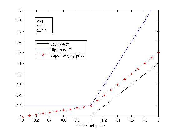
(I) If  $\Delta>0,\,\Delta<K$

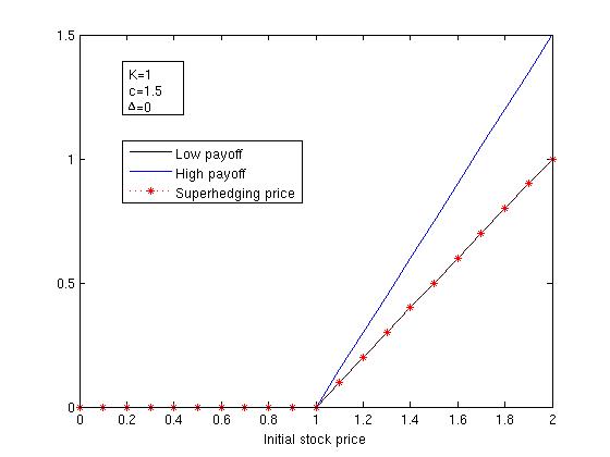
(II) If  $\Delta=0,\,c>1$

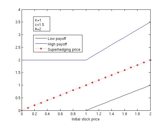
(III) If   $\Delta\geq K$

Figure 1. Call option

Example 4.8 (Put option).

Let $K>0$ be a constant. Consider a game put option

$$f_{1}(S_{t})=(K-S_{t})^{+},\quad f_{2}(S_{t})=c(K-S_{t})^{+}+\Delta.$$

We distinguish between two cases.

1. $\Delta<K$:  In this case $A=K$, $\beta=\frac{\Delta-K}{K}<m=0$ and $\rho=\infty$. Hence, see Figure 2I and Figure 2II, the super-replication price is

   $$g(S_{0})=\Big{(}K-\frac{K-\Delta}{K}S_{0}\Big{)}\,\mathbb{I}_{S_{0}<K}+\Delta\,\mathbb{I}_{S_{0}\geq K}.$$

   1. If $S_{0}<K$, then $(\hat{\pi},\hat{\sigma})=\big{(}(K-\frac{K-\Delta}{K}S_{0},-\frac{K-\Delta}{K}),\,\inf\{t:S_{t}=K\}\wedge T\big{)}.$

   2. If $S_{0}\geq K$, then $(\hat{\pi},\hat{\sigma})=\big{(}(\Delta,0),0\big{)}$.

2. $\Delta\geq K$  In this case,

   $$A=\left\{\begin{array}[]{ll}K&\mbox{if }\ \Delta=K\\ \infty&\mbox{if }\ \Delta>K,\end{array}\right.$$

   and

   $$\beta=\left\{\begin{array}[]{ll}0&\mbox{if }\ \Delta=K\\ \infty&\mbox{if }\ \Delta>K.\end{array}\right.$$

   Thus $\beta\geq m=0$. Hence, see Figure 2III, the super-replication price equals $g(S_{0})\equiv K$, and $(\hat{\pi},\hat{\sigma})=\big{(}(K,0),T\big{)}$.

In the Put-case, the super-replication price is independent of the scaling factor $c\geq 1$.

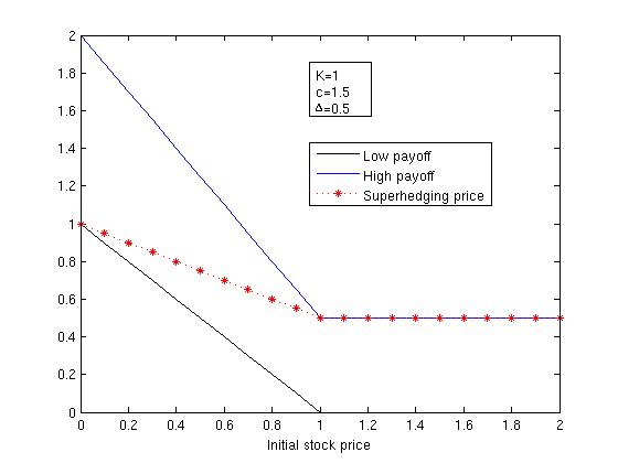
(I) If  $\Delta>0,\,\Delta<K$

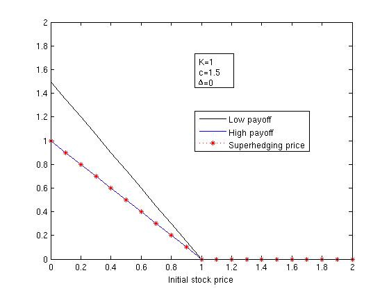
(II) If  $\Delta=0,\,c>1$

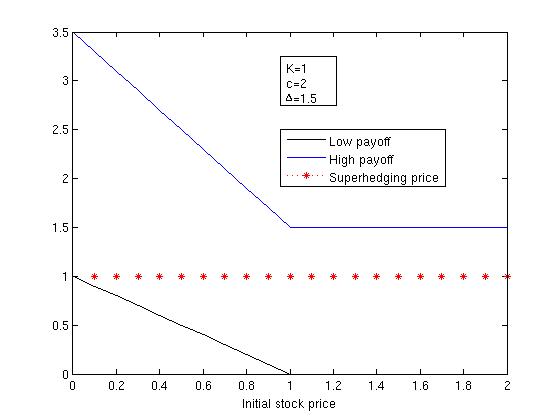
(III) If  $\Delta\geq K$

Figure 2. Put option

Example 4.9 (Power option).

Let $p>1$ and consider the game $p$-th power option

$$f_{1}(S_{t})=S_{t}^{p},\quad f_{2}(S_{t})=cS_{t}^{p}+\Delta.$$

We have $\rho=m=\infty$ and when $\Delta>0$, $A=\left(\frac{\Delta}{c(p-1)}\right)^{1/p}$, $\beta=cp\left(\frac{\Delta}{c(p-1)}\right)^{1-1/p}$. Thus, see Figure 3I and Figure 3II, the super–replication price equals

$$g(S_{0})=\beta S_{0}\,\mathbb{I}_{S_{0}<A}+(cS_{0}^{p}+\Delta)\,\mathbb{I}_{S_{0}\geq A}.$$

The cheapest super-replicating strategy is given by:

If $S_{0}<A$, then $(\hat{\pi},\hat{\sigma})=\big{(}(\beta S_{0},\beta),\,\inf\{t:S_{t}=A\}\wedge T\big{)}$.

If $S_{0}\geq A$, then $(\hat{\pi},\hat{\sigma})=\big{(}(cS_{0}^{p}+\Delta,0),0\big{)}$.

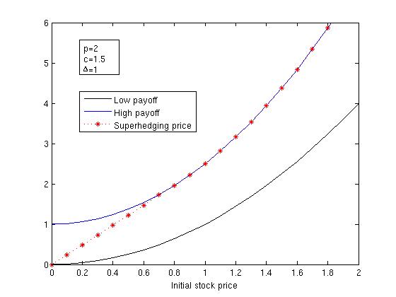
(I) If $\Delta>0$

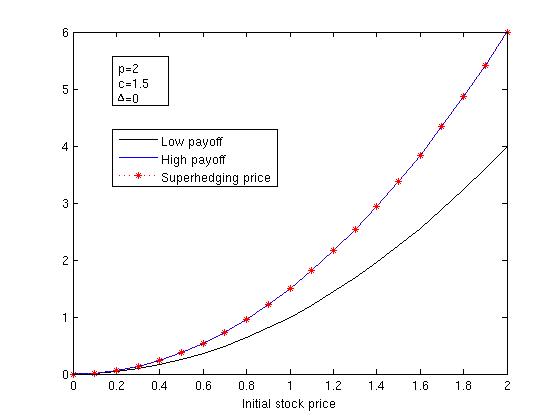
(II) If $\Delta=0,\,c>1$

Figure 3. Power option

5. Proof of Proposition 2.3

Proof.

Let $\alpha\in\mathcal{C}(\nu_{0})$ and $\epsilon>0$. We will show (for both set-ups I and II) that there exists a probability measure $\mathbb{Q}\ll\mathbb{P}$ such that the properties of Definition 2.1 hold true.
I. There is a constant $C>0$ such that $\frac{1}{C}\leq\alpha\leq C$. Without loss of generality we assume that $\epsilon<\frac{1}{2C}.$ Define the stopping time

$$\Theta=\inf\{t:|\alpha_{t}-\nu_{t}|\geq\epsilon\}\wedge T.$$

Clearly,

$$0<\frac{1}{2C}\leq\inf_{0\leq t\leq\Theta}\nu_{t}\leq\sup_{0\leq t\leq\Theta}\nu_{t}\leq C+\frac{1}{2C}.$$

From the assumptions on the functions $a,b,c$, we get that there exists a constant $\tilde{C}>0$ such that

(5.1) $$\sup_{0\leq t\leq\Theta}\left[|a(t,\nu_{t})|+|b(t,\nu_{t})|+|c(t,\nu_{t})|+\frac{1}{|b(t,\nu_{t})|}\right]\leq\tilde{C}.$$

Fix $n>\frac{2\tilde{C}}{T}$. For $k=1,...,n$, let

$$I_{k} =\int_{(k-1)T/n}^{kT/n}a(t,\nu_{t})\,dt+\int_{(k-1)T/n}^{kT/n}c(t,\nu_{t})\,dW_{t},$$

$$J_{k} =\alpha_{\frac{kT}{n}}-\alpha_{\frac{(k-1)T}{n}}.$$

Introduce the function $\Phi(x)=-n^{2}\vee(x\wedge n^{2})$, $x\in\mathbb{R}$. Let ${\{\gamma_{t}\}}_{t=0}^{T}$ and ${\{\tilde{W}_{t}\}}_{t=0}^{T}$ be the unique stochastic processes which satisfy the following (recursive) relations:

$$\hat{W}_{t}=\tilde{W}_{t}+\int_{0}^{t}\gamma_{u}\,du$$

where $\gamma_{t}=0$ for $t\leq\frac{T}{n}$, and for $k=1,...,n-1$

$$\gamma_{t}=\Phi\left(\frac{n}{b(t,\nu_{t})T}\Big{(}J_{k}-I_{k}-\int_{(k-1)T/n}^{kT/n}b(u,\nu_{u})\,d\tilde{W}_{u}\Big{)}\right),\ \frac{kT}{n}<t\leq\frac{(k+1)T}{n}.$$

The process $\{\gamma_{t}\}_{t=0}^{T}$ is uniformly bounded, thus we deduce from the Girsanov theorem and Novikov condition that there exists a probability measure $\mathbb{Q}\sim\mathbb{P}$ (which depends on $n$) such that $\{(\tilde{W}_{t},W_{t})\}_{t=0}^{T}$ is a two dimensional standard Brownian motion with respect to $\mathbb{Q}$ and the filtration ${\{\mathcal{F}_{t}\}}_{t=0}^{T}$.

For any $k=1,...,n$, denote $L_{k}=\int_{(k-1)T/n}^{kT/n}b(t,\nu_{t})\,d\tilde{W}_{t}$ and introduce the event

$$A_{k}=\{kT/n<\Theta\}\cap\left\{|I_{k}|+|L_{k}|>1\right\}.$$

Clearly, for any $k=1,...,n$

$$\mathbb{I}_{\frac{kT}{n}<\Theta}\,|I_{k}|\leq\Big{|}\int_{(k-1)T/n}^{kT/n}\mathbb{I}_{t<\Theta}\,a(t,\nu_{t})\,dt\Big{|}+\Big{|}\int_{(k-1)T/n}^{kT/n}\mathbb{I}_{t<\Theta}\,c(t,\nu_{t})\,dW_{t}\Big{|}.$$

This together with (5.1) and the Burkholder–Davis–Gundy inequality yield that for any $p>1$ there exists a constant $c_{p}>0$ such that

(5.2) $$\mathbb{E}_{\mathbb{Q}}\left[\mathbb{I}_{\frac{kT}{n}<\Theta}\,|I_{k}|^{p}\right]\leq 2^{p}\Big{(}(\tilde{C}T/n)^{p}+c_{p}(\tilde{C}^{2}T/n)^{p/2}\Big{)}.$$

Similarly,

(5.3) $$\mathbb{E}_{\mathbb{Q}}\left[\mathbb{I}_{\frac{kT}{n}<\Theta}|L_{k}|^{p}\right]\leq\mathbb{E}_{\mathbb{Q}}\left[\Big{|}\int_{(k-1)T/n}^{kT/n}\mathbb{I}_{t<\Theta}b(t,\nu_{t})\,d\tilde{W}_{t}\Big{|}^{p}\right]\leq c_{p}(\tilde{C}^{2}T/n)^{p/2}.$$

By applying the Markov inequality and (5.2)–(5.3) for $p=4$, we obtain

(5.4) $$\mathbb{Q}\big{(}\cup_{k=1}^{n}A_{k}\big{)}\leq\sum_{k=1}^{n}\mathbb{Q}(A_{k})\leq\frac{c}{n}$$

for some constant $c$ (independent of $n$).

Next, let $k<n$ and $kT/n\leq t<(k+1)T/n$. Consider the event

$$U:=\{t<\Theta\}\setminus\Big{(}\big{(}\cup_{j=1}^{n}A_{j}\big{)}\cup\big{(}\max_{|u-v|\leq\frac{T}{n}}|\alpha_{u}-\alpha_{v}|>1\big{)}\Big{)}.$$

Recall the constant $\tilde{C}$ from (5.1). As $n>\frac{2\tilde{C}}{T}$, we get on the event $U$ that for any $u\leq t$

$$\gamma_{u}b(u,\nu_{u})=\frac{n(J_{m}-I_{m}-L_{m})}{T},\quad\mbox{for }\ \frac{mT}{n}<u\leq\frac{(m+1)T}{n},$$

where we set $I_{0}=J_{0}=L_{0}=0$. Thus, on the event $U$ we have

$$\nu_{\frac{kT}{n}}-\alpha_{\frac{kT}{n}}=\sum_{m=1}^{k}[I_{m}+L_{m}-J_{m}]+\sum_{m=1}^{k-1}[J_{m}-I_{m}-L_{m}]=\mathbb{I}_{\frac{kT}{n}<\Theta}(I_{k}+L_{k}-J_{k})$$

as well as

$$|\nu_{t}-\nu_{\frac{kT}{n}}| \leq\Big{|}\int_{kT/n}^{t}\mathbb{I}_{u<\Theta}\,a(u,\nu_{u})\,du\Big{|}+\Big{|}\int_{kT/n}^{t}\mathbb{I}_{u<\Theta}\,b(u,\nu_{u})\,d\tilde{W}_{u}\Big{|}$$

$$\quad+\Big{|}\int_{kT/n}^{t}\mathbb{I}_{u<\Theta}\,c(u,\nu_{u})\,dW_{u}\Big{|}+\mathbb{I}_{\frac{kT}{n}<\Theta}\,(|J_{k}|+|I_{k}|+|L_{k}|).$$

We conclude that on the event $\hat{U}:=\Omega\setminus\Big{(}\big{(}\cup_{j=1}^{n}A_{j}\big{)}\cup\big{(}\max_{|u-v|\leq\frac{T}{n}}|\alpha_{u}-\alpha_{v}|>1\big{)}\Big{)}$

(5.5) $$\sup_{0\leq t<\Theta}|\alpha_{t}-\nu_{t}|$$

$$\leq \,\max_{|u-v|\leq\frac{T}{n}}|\alpha_{u}-\alpha_{v}|+2\max_{1\leq k\leq n}\Big{(}\mathbb{I}_{\frac{kT}{n}<\Theta}\,(|J_{k}|+|I_{k}|+|L_{k}|)\Big{)}+\max_{1\leq k\leq n}(\Gamma_{k}+\Upsilon_{k}+\Lambda_{k})$$

$$\leq \,3\max_{|u-v|\leq\frac{T}{n}}|\alpha_{u}-\alpha_{v}|+2\max_{1\leq k\leq n}\Big{(}\mathbb{I}_{\frac{kT}{n}<\Theta}\,(|I_{k}|+|L_{k}|)\Big{)}+\max_{1\leq k\leq n}(\Gamma_{k}+\Upsilon_{k}+\Lambda_{k}),$$

where

$$\Gamma_{k} =\max_{(k-1)T/n\leq t\leq kT/n}\Big{|}\int_{(k-1)T/n}^{t}\mathbb{I}_{u<\Theta}\,a(u,\nu_{u})\,du\Big{|},$$

$$\Upsilon_{k} =\max_{(k-1)T/n\leq t\leq kT/n}\Big{|}\int_{(k-1)T/n}^{t}\mathbb{I}_{u<\Theta}\,b(u,\nu_{u})\,d\tilde{W}_{u}\Big{|},$$

$$\Lambda_{k} =\max_{(k-1)T/n\leq t\leq kT/n}\Big{|}\int_{(k-1)T/n}^{t}\mathbb{I}_{u<\Theta}\,c(u,\nu_{u})\,dW_{u}\Big{|}.$$

Similarly to (5.2)–(5.3), we get that

$$\mathbb{E}_{\mathbb{Q}}\left[\max_{1\leq k\leq n}(\Gamma_{k}+\Upsilon_{k}+\Lambda_{k})^{4}\right]\leq 3^{4}\sum_{k=1}^{n}\mathbb{E}_{\mathbb{Q}}\big{[}\Gamma^{4}_{k}+\Upsilon^{4}_{k}+\Lambda^{4}_{k}\big{]}\leq\frac{\tilde{c}}{n}$$

for some constant $\tilde{c}$. Thus, from the Markov inequality we get that for sufficiently large $n$

(5.6) $$\mathbb{Q}\left(\max_{1\leq k\leq n}[\Gamma_{k}+\Upsilon_{k}+\Lambda_{k}]\geq\frac{\epsilon}{3}\right)<\frac{\epsilon}{5}.$$

Similarly, (5.2)–(5.3) give that for sufficiently large $n$

(5.7) $$\mathbb{Q}\left(2\max_{1\leq k\leq n}\left[\mathbb{I}_{\frac{kT}{n}<\Theta}(|I_{k}|+|L_{k}|)\right]\geq\frac{\epsilon}{3}\right)<\frac{\epsilon}{5}.$$

The stochastic process $\alpha$ is progressively measurable with respect to the filtration generated by $W$, thus the distribution of $\alpha$ under $\mathbb{Q}$ is the same as under $\mathbb{P}$ and so, for sufficiently large $n$

(5.8) $$\mathbb{Q}\Big{(}3\max_{|u-v|\leq\frac{T}{n}}|\alpha_{u}-\alpha_{v}|\geq\frac{\epsilon}{3}\Big{)}<\frac{\epsilon}{5}.$$

Finally, by combining (5.4)–(5.8), we obtain that for sufficiently large $n$,

$$\ \mathbb{Q}(\|\alpha-\nu\|_{\infty}>\epsilon)$$

$$\leq \ \mathbb{Q}\Big{(}\big{(}\cup_{j=1}^{n}A_{j}\big{)}\cup\big{(}\max_{|u-v|\leq\frac{T}{n}}|\alpha_{u}-\alpha_{v}|>1\big{)}\Big{)}+\mathbb{Q}\Big{(}\big{(}\sup_{0\leq t<\Theta}|\alpha_{t}-\nu_{t}|=\epsilon\big{)}\cap\hat{U}\Big{)}$$

$$\leq \ \frac{c}{n}+\frac{\epsilon}{5}+\frac{3\epsilon}{5}<\epsilon,$$

as required.∎
II. Consider the continuous stochastic process $\phi_{t}=\ln\alpha_{t}-\ln\nu^{(1)}_{t}$, $t\in[0,T]$. Fix $\delta>0$. Choose $n\in\mathbb{N}$ sufficiently large such that

(5.9) $$\mathbb{P}\Big{(}\max_{|u-v|\leq\frac{T}{n}}|\phi_{u}-\phi_{v}|\geq\delta\Big{)}\leq\delta.$$

For $k=0,...,n-1$, define the events

$$\hat{A}_{k}=\left\{\max_{kT/n\leq t\leq(k+1)T/n}|\ln\nu^{(2)}_{t}-\ln\nu^{(2)}_{\frac{kT}{n}}-(nt/T-k)(\phi_{\frac{kT}{n}}-\phi_{\frac{(k-1)T}{n}})|<\frac{\delta}{n}\right\}$$

where we set $\phi_{-\frac{T}{n}}\equiv\phi_{0}$. First, we argue that for any $k$

(5.10) $$\mathbb{P}(\hat{A}_{k}\,|\,\mathcal{F}_{\frac{kT}{n}})>0\ \mbox{a.s.}$$

Denote by $\{\mathbf{G}_{t}\}_{t=0}^{T}$ the usual augmentation of the filtration generated by $\nu^{(2)}$. By our assumptions, $\nu^{(2)}$ is independent of $W$ and $\phi$. This, together with the fact that $\{\mathcal{F}_{t}\}_{t=0}^{T}$ is the usual augmentation of the filtration generated by $W$ and $\nu^{(2)}$ yields

$$\mathbb{P}\left(\hat{A}_{k}|\mathcal{F}_{\frac{kT}{n}}\right)=\Psi\left(\phi_{\frac{(k-1)T}{n}},\phi_{\frac{kT}{n}},\nu^{(2)}\right)\ \mbox{ a.s.,}$$

where $\Psi:\mathbb{R}\times\mathbb{R}\times C_{+}[0,T]\rightarrow\mathbb{R}$ is a measurable function satisfying a.s.

$$\Psi(u,v,\nu^{(2)})=\mathbb{P}\left(\max_{kT/n\leq t\leq(k+1)T/n}|\ln\nu^{(2)}_{t}-\ln\nu^{(2)}_{\frac{kT}{n}}-\right.\\ \left.(nt/T-k)(v-u)|<\frac{\delta}{n}\,\big{|}\,\mathbf{G}_{\frac{kT}{n}}\right).$$

It is assumed $\ln\nu^{(2)}$ satisfies the CFS property with respect to its natural filtration. We deduce from Pakkanen (2010, Lemma 2.3) that $\ln\nu^{(2)}$ satisfies the CFS property with respect to the usual augmented filtration $\{\mathbf{G}_{t}\}_{t=0}^{T}$, as well. Therefore, we obtain that $\Psi(u,v,\nu^{(2)})>0\ \mathbb{P}$-a.s., for any $u,v\in\mathbb{R}$, hence we conclude that (5.10) holds true.

Next, define the continuous martingale $\mathbf{Z}=\{\mathbf{Z}_{t}\}_{t=0}^{T}$ by $\mathbf{Z}_{0}=1$ and

$$\mathbf{Z}_{t}=\frac{\mathbb{P}\big{(}\hat{A}_{k}\,|\,\mathcal{F}_{t}\big{)}}{\mathbb{P}\big{(}\hat{A}_{k}\,|\,\mathcal{F}_{\frac{kT}{n}}\big{)}}\sum_{i=0}^{k-1}\frac{\mathbb{I}_{\hat{A}_{i}}}{\mathbb{P}\big{(}\hat{A}_{i}\,|\,\mathcal{F}_{\frac{iT}{n}}\big{)}},\ \ t\in(kT/n,(k+1)T/n],\ \ 0\leq k\leq n-1.$$

There exists a probability measure $\mathbb{Q}\ll\mathbb{P}$ such that $\frac{d\mathbb{Q}}{d\mathbb{P}}{|}_{\mathcal{F}_{t}}=\mathbf{Z}_{t}$, $t\in[0,T]$. Let us prove that (for sufficiently small $\delta>0$), $\mathbb{Q}$ satisfies the required properties. Fix $k<n$ and $t\in[kT/n,(k+1)T/n]$. On the event $\mathbf{Z}_{t}\neq 0$, using that $W_{\frac{(k+1)T}{n}}-W_{t}$ is independent of $\mathcal{F}_{t}$ and $\hat{A}_{k}$, yields

$$\mathbb{E}_{\mathbb{Q}}\left(W_{\frac{(k+1)T}{n}}-W_{t}\,|\,\mathcal{F}_{t}\right) =\frac{1}{\mathbf{Z}_{t}}\mathbb{E}_{\mathbb{P}}\left(\mathbf{Z}_{\frac{(k+1)T}{n}}(W_{\frac{(k+1)T}{n}}-W_{t})\,|\,\mathcal{F}_{t}\right)$$

$$=\frac{1}{P(\hat{A}_{k}|\mathcal{F}_{t})}\mathbb{E}_{\mathbb{P}}\left(\mathbb{I}_{\hat{A}_{k}}(W_{\frac{(k+1)T}{n}}-W_{t})\,|\,\mathcal{F}_{t}\right)$$

$$=0.$$

Thus, for any $k<n$ the stochastic process $\{W_{t}\}_{t=kT/n}^{(k+1)T/n}$ is a $\mathbb{Q}$-martingale, and so $W=\{W_{t}\}_{t=0}^{T}$ is a $\mathbb{Q}$-martingale. As $\mathbb{Q}\ll\mathbb{P}$, we conclude that $\langle W\rangle_{t}\equiv t$, $\mathbb{Q}$-a.s. This together with Lévy’s characterization theorem yields that $W$ is a Brownian motion with respect to $\mathbb{Q}$ and $\{\mathcal{F}_{t}\}_{t=0}^{T}$.

We arrive to the final step of the proof. Consider the event

$$\hat{A}:=\Big{(}\bigcap_{i=0}^{n-1}\hat{A}_{i}\Big{)}\cap\Big{\{}\max_{|u-v|\leq\frac{T}{n}}|\phi_{u}-\phi_{v}|\leq\delta\Big{\}}.$$

The stochastic process $\phi$ is adapted to the filtration generated by $W$; in particular, $\phi$ is determined by $\{W_{t}\}_{t=0}^{T}$. Hence ($W$ is a Brownian motion under $\mathbb{P}$ and $\mathbb{Q}$), the distributions of $\phi$ under $\mathbb{P}$ and $\mathbb{Q}$ are the same. This, together with (5.9) and the fact that $\mathbb{Q}\big{(}\bigcap_{i=0}^{n-1}\hat{A}_{i}\big{)}=1$ yields

(5.11) $$\mathbb{Q}(\hat{A})=\mathbb{Q}\Big{(}\max_{|u-v|\leq\frac{T}{n}}|\phi_{u}-\phi_{v}|\leq\delta\Big{)}=\mathbb{P}\Big{(}\max_{|u-v|\leq\frac{T}{n}}|\phi_{u}-\phi_{v}|\leq\delta\Big{)}\geq 1-\delta.$$

Next, let $k<n$ and $t\in[kT/n,(k+1)T/n]$. Observe that $\phi_{0}=\ln\nu^{(2)}_{0}$. Thus, we have on the event $\hat{A}$

$$|\ln\nu_{t}-\ln\alpha_{t}| =|\ln\nu^{(2)}_{t}-\phi_{t}|$$

$$\leq\sum_{i=0}^{k-1}\left|\ln\nu^{(2)}_{\frac{(i+1)T}{n}}-\ln\nu^{(2)}_{\frac{iT}{n}}-\phi_{\frac{iT}{n}}+\phi_{\frac{(i-1)T}{n}}\right|$$

$$\quad+|\phi_{\frac{kT}{n}}-\phi_{\frac{(k-1)T}{n}}|+|\phi_{t}-\phi_{\frac{kT}{n}}|+|\ln\nu^{(2)}_{t}-\ln\nu^{(2)}_{\frac{kT}{n}}|$$

$$\leq\frac{\delta k}{n}+2\delta+\frac{\delta}{n}+\delta+(nt/T-k)\delta$$

$$\leq 6\delta.$$

From the inequality

$$|e^{x}-e^{y}|\leq e^{\max(x,y)}|x-y|\leq e^{x}e^{|x-y|}|x-y|\ \ x,y\in\mathbb{R}$$

we conclude that on the event $\hat{A}$, (take $x=\ln\alpha_{t}$, $y=\ln\nu_{t}$)

$$\sup_{0\leq t\leq T}|\alpha_{t}-\nu_{t}|\leq 6\delta e^{6\delta}||\alpha||_{\infty}.$$

This, together with applying (5.11) for sufficiently small $\delta>0$ (recall that $\alpha$ is uniformly bounded) we get $\mathbb{Q}\left(||\alpha-\nu||_{\infty}<\epsilon\right)>1-\epsilon,$ and the proof is completed. ∎

6. Proof of Theorem 4.2

In this section, we finish the proof of Theorem 4.2 by showing that the inequality (4.6) holds true. It suffices to show that for any super-replicating strategy $(\pi,\sigma)$ we have the inequality

(6.1) $$Z^{\pi}_{0}\geq g(S_{0}).$$

To this end, let $(\pi,\sigma)$ be a super-replicating strategy. Choose $\epsilon>0$. The stochastic process ${\{r_{t}\}}_{t=0}^{T}$ is uniformly bounded, thus there exists $\mathbf{T}<T$ such that

(6.2) $$\int_{0}^{\mathbf{T}}r_{t}\,dt<\epsilon.$$

Let ${\{\mathcal{G}_{t}\}}_{t=0}^{\mathbf{T}}$ be the filtration generated by $W$ and completed by the null sets. Denote by ${\mathcal{T}}_{\mathbf{T}}$ the set of all stopping times with respect to the filtration ${\{\mathcal{G}_{t}\}}_{t=0}^{\mathbf{T}}$ with values in $[0,\mathbf{T}]$. By Corollary 7.3, there exists a stochastic process $\alpha\in\mathcal{C}(\nu_{0})$ such that

(6.3) $$\inf_{\zeta\in{\mathcal{T}}_{\mathbf{T}}}\mathbb{E}_{\mathbb{P}}\Big{[}f_{2}(\mathbf{S}^{(\alpha)}_{\zeta})\mathbb{I}_{\zeta<\mathbf{T}}+f_{1}(\mathbf{S}^{(\alpha)}_{\mathbf{T}})\mathbb{I}_{\zeta=\mathbf{T}}\Big{]}>g(S_{0})-\epsilon,$$

where

$$\mathbf{S}^{(\alpha)}_{t}=S_{0}e^{\int_{0}^{t}\alpha_{u}dW_{u}-\frac{1}{2}\int_{0}^{t}\alpha^{2}_{u}du},\ \ t\in[0,T].$$

Choose $\delta>0$. The financial market is fully incomplete. Hence by definition, we obtain a probability measure $\mathbb{Q}\ll\mathbb{P}$ such that

(6.4) $$\mathbb{Q}\big{(}\|\alpha-\nu\|_{\infty}\geq\delta\big{)}<\delta$$

and that $W$ is a Brownian motion with respect to $\mathbb{Q}$ and $\{\mathcal{F}_{t}\}_{t=0}^{T}$.

Define the stopping time $\tau=\mathbf{\inf}\{t:|\alpha_{t}-\nu_{t}|\geq\delta\}\wedge\mathbf{T}$ and denote $\pi=(Z^{\pi}_{0},\gamma)$. From (4.3)–(4.4), it follows that the stochastic integral

$$\int_{0}^{t\wedge\sigma}\gamma_{u}\tilde{S}_{u}\nu_{u}\,dW_{u},\ \ t\in[0,T]$$

is uniformly bounded from below, and so it is a supermartingale with respect to the probability measure $\mathbb{Q}$. Thus, from (4.3)–(4.4)

$$\mathbb{E}_{\mathbb{Q}}\left[\frac{B_{0}}{B_{\sigma\wedge\tau}}\big{(}f_{2}(S_{\sigma})\mathbb{I}_{\sigma<\tau}+f_{1}(S_{\tau})\mathbb{I}_{\tau\leq\sigma}\big{)}\right]\leq\mathbb{E}_{\mathbb{Q}}\left[\frac{B_{0}}{B_{\sigma\wedge\tau}}Z^{\pi}_{\sigma\wedge\tau}\right]\leq Z^{\pi}_{0},$$

and so from (6.2), we conclude that

(6.5) $$e^{\epsilon}Z^{\pi}_{0}\geq\mathbb{E}_{\mathbb{Q}}\big{[}f_{2}(S_{\sigma})\mathbb{I}_{\sigma<\tau}+f_{1}(S_{\tau})\mathbb{I}_{\tau\leq\sigma}\big{]}.$$

Clearly,

$$\int_{0}^{\sigma\wedge\tau}|\alpha^{2}_{t}-\nu^{2}_{t}|dt\leq\delta(2||\alpha||_{\infty}+\delta)T,$$

and from Itô’s Isometry

$$\mathbb{E}_{\mathbb{Q}}\left[\Big{(}\int_{0}^{\sigma\wedge\tau}(\nu_{t}-\alpha_{t})\,dW_{t}\Big{)}^{2}\right]\leq\delta^{2}T.$$

Thus, from the Markov inequality we get for sufficiently small $\delta$

(6.6) $$\mathbb{Q}\left(\int_{0}^{\sigma\wedge\tau}|\alpha^{2}_{t}-\nu^{2}_{t}|\,dt+\Big{|}\int_{0}^{\sigma\wedge\tau}(\nu_{t}-\alpha_{t})\,dW_{t}\Big{|}>2\sqrt{\delta}\right)<c\sqrt{\delta}$$

for some constant $c>0$ (which may depend on the chosen $\epsilon>0$). The SDE (2.2) implies that

$$S_{\sigma\wedge\tau}=S_{0}e^{\int_{0}^{\sigma\wedge\tau}\nu_{t}dW_{t}+\int_{0}^{\sigma\wedge\tau}(r_{t}-\nu^{2}_{t}/2)dt}.$$

From (6.2) and (6.6) we get that for sufficiently small $\delta$

(6.7) $$\mathbb{Q}\left(|\ln S_{\sigma\wedge\tau}-\ln\mathbf{S}^{(\alpha)}_{\sigma\wedge\tau}|>2\epsilon\right)<c\sqrt{\delta}.$$

Now, we arrive at the final step of the proof. Set

$$\tilde{\sigma}=\sigma\wedge\mathbf{T},\ \quad X=\sup_{0\leq t\leq T}f_{2}(\mathbf{S}^{(\alpha)}_{t}),$$

and introduce the event $U=(\tau<\mathbf{T})\cup(|\ln S_{\sigma\wedge\tau}-\ln\mathbf{S}^{(\alpha)}_{\sigma\wedge\tau}|>2\epsilon).$ We deduce from (2.4) that

(6.8) $$|\ln x-\ln y|\leq 2\epsilon\Rightarrow f_{i}(y)\geq\frac{(1-L(e^{2\epsilon}-1))f_{i}(x)-Lx(e^{2\epsilon}-1)}{1+L(e^{2\epsilon}-1)},\ \ i=1,2.$$

From (6.5) and (6.8) we obtain

(6.9) $$e^{\epsilon}Z^{\pi}_{0} \geq\mathbb{E}_{\mathbb{Q}}\big{[}\mathbb{I}_{\Omega\setminus U}\left(f_{2}(S_{\tilde{\sigma}})\mathbb{I}_{\tilde{\sigma}<\mathbf{T}}+f_{1}(S_{\mathbf{T}})\mathbb{I}_{\tilde{\sigma}=\mathbf{T}}\right)\big{]}$$

$$\geq\frac{1-L(e^{2\epsilon}-1)}{1+L(e^{2\epsilon}-1)}\,\mathbb{E}_{\mathbb{Q}}\left[\mathbb{I}_{\Omega\setminus U}\left(f_{2}(\mathbf{S}^{(\alpha)}_{\tilde{\sigma}})\mathbb{I}_{\tilde{\sigma}<\mathbf{T}}+f_{1}(\mathbf{S}^{(\alpha)}_{\mathbf{T}})\mathbb{I}_{\tilde{\sigma}=\mathbf{T}}\right)\right]$$

$$\phantom{\geq}\ -\frac{L(e^{2\epsilon}-1)}{1+L(e^{2\epsilon}-1)}\,\mathbb{E}_{\mathbb{Q}}[\mathbf{S}^{(\alpha)}_{\tilde{\sigma}}]$$

$$\geq\frac{1-L(e^{2\epsilon}-1)}{1+L(e^{2\epsilon}-1)}\,\mathbb{E}_{\mathbb{Q}}\left[f_{2}(\mathbf{S}^{(\alpha)}_{\tilde{\sigma}})\mathbb{I}_{\tilde{\sigma}<\mathbf{T}}+f_{1}(\mathbf{S}^{(\alpha)}_{\mathbf{T}})\mathbb{I}_{\tilde{\sigma}=\mathbf{T}}\right]$$

$$\phantom{\geq}\ -\frac{1-L(e^{2\epsilon}-1)}{1+L(e^{2\epsilon}-1)}\,\mathbb{E}_{\mathbb{Q}}[\mathbb{I}_{U}X]-\frac{LS_{0}(e^{2\epsilon}-1)}{1+L(e^{2\epsilon}-1)}.$$

The growth condition (4.2) implies that $\mathbb{E}_{\mathbb{Q}}[X^{2}]<\infty$. Observe that $(\tau<\mathbf{T})\subset(\|\alpha-\nu\|_{\infty}\geq\delta)$. Thus, from the Cauchy-–Schwarz inequality, (6.4) and (6.7), we get that for sufficiently small $\delta>0$

(6.10) $$\mathbb{E}_{\mathbb{Q}}[\mathbb{I}_{U}X]\leq\left(\mathbb{E}_{\mathbb{Q}}[X^{2}]\right)^{1/2}\left(\delta+c\sqrt{\delta}\right)^{1/2}<\epsilon.$$

Finally, we estimate $\mathbb{E}_{\mathbb{Q}}\left[f_{2}(\mathbf{S}^{(\alpha)}_{\tilde{\sigma}})\mathbb{I}_{\tilde{\sigma}<\mathbf{T}}+f_{1}(\mathbf{S}^{(\alpha)}_{\mathbf{T}})\mathbb{I}_{\tilde{\sigma}=\mathbf{T}}\right]$. Denote by $\mathbb{T}$ the set of all stopping times with respect to the filtration $\{\mathcal{F}_{t}\}_{t=0}^{T}$ with values in $[0,\mathbf{T}]$. The stochastic process $W$ is a Brownian motion under the probability measure $\mathbb{Q}$ and the filtration ${\{\mathcal{F}_{t}\}}_{t=0}^{T}$. Thus, from the Markov property of Brownian motion, the fact that $\alpha$ is adapted to the filtration $\{\mathcal{G}_{t}\}_{t=0}^{T}$, $\tilde{\sigma}\in\mathbb{T}$ and (6.3), it follows that

$$\mathbb{E}_{\mathbb{Q}}\left[f_{2}(\mathbf{S}^{(\alpha)}_{\tilde{\sigma}})\mathbb{I}_{\tilde{\sigma}<\mathbf{T}}+f_{1}(\mathbf{S}^{(\alpha)}_{\mathbf{T}})\mathbb{I}_{\tilde{\sigma}=\mathbf{T}}\right]\geq \inf_{\zeta\in{\mathbb{T}}}\mathbb{E}_{\mathbb{Q}}\Big{[}f_{2}(\mathbf{S}^{(\alpha)}_{\zeta})\mathbb{I}_{\zeta<\mathbf{T}}+f_{1}(\mathbf{S}^{(\alpha)}_{\mathbf{T}})\mathbb{I}_{\zeta=\mathbf{T}}\Big{]}$$

$$= \inf_{\zeta\in\mathcal{T}_{\mathbf{T}}}\mathbb{E}_{\mathbb{Q}}\Big{[}f_{2}(\mathbf{S}^{(\alpha)}_{\zeta})\mathbb{I}_{\zeta<\mathbf{T}}+f_{1}(\mathbf{S}^{(\alpha)}_{\mathbf{T}})\mathbb{I}_{\zeta=\mathbf{T}}\Big{]}$$

$$= \inf_{\zeta\in{\mathcal{T}}_{\mathbf{T}}}\mathbb{E}_{\mathbb{P}}\Big{[}f_{2}(\mathbf{S}^{(\alpha)}_{\zeta})\mathbb{I}_{\zeta<\mathbf{T}}+f_{1}(\mathbf{S}^{(\alpha)}_{\mathbf{T}})\mathbb{I}_{\zeta=\mathbf{T}}\Big{]}$$

$$> \,g(S_{0})-\epsilon.$$

This together with (6.9)–(6.10) gives

$$e^{\epsilon}Z^{\pi}_{0}\geq\frac{1-L(e^{2\epsilon}-1)}{1+L(e^{2\epsilon}-1)}(g(S_{0})-\epsilon)-\frac{1-L(e^{2\epsilon}-1)}{1+L(e^{2\epsilon}-1)}\epsilon-\frac{LS_{0}(e^{2\epsilon}-1)}{1+L(e^{2\epsilon}-1)},$$

and by letting $\epsilon\downarrow 0$ we obtain (6.1). ∎

Remark 6.1.

A natural question is whether for game options with path dependent payoffs the model free super–replication price is equal to the price achieved in fully incomplete markets (see Remark 4.3). In order to answer this question we should develop a dual characterization for the super–replication price of path dependent game options in a model free setup. This was not done so far.

7. Auxiliary lemmas for the proof of Theorem 4.2

The goal of this section is to establish Corollary 7.3 which provides a connection between the function $g$ (which is the game variant of a concave envelope) and the left hand side of (7.6) which can be viewed as an optimal stopping problem under volatility uncertainty.

Consider the probability space $(\Omega,{\mathcal{F}},{\mathbb{P}})$ and the filtration $\{\mathcal{G}_{t}\}_{t=0}^{T}$ generated by the Brownian motion $\{W_{t}\}_{t=0}^{T}$, completed by the null sets. For any $u\in[0,T]$ we denote by $\mathcal{T}_{u}$ the set of all stopping times with respect to the filtration $\{\mathcal{G}_{t}\}_{t=0}^{T}$ with values in $[0,u]$. For any $x>0$ and any (sufficiently integrable) progressively measurable process $\alpha=\{\alpha_{t}\}_{t=0}^{T}$ (with respect to $\{\mathcal{G}_{t}\}_{t=0}^{T}$) define the process

$$\mathbf{S}^{\alpha,x}_{t}=xe^{\int_{0}^{t}\alpha_{v}dW_{v}-\frac{1}{2}\int_{0}^{t}\alpha^{2}_{v}dv},\ \ t\in[0,T].$$

Denote by $\mathcal{A}$ the set of all non–negative, progressively measurable processes $\alpha=\{\alpha_{t}\}_{t=0}^{T}$ with $\int_{0}^{T}\alpha^{2}_{t}\,dt<\infty$   a.s. which satisfy the following: there exists a constant $C=C(\alpha)$ such that $\frac{1}{C}\leq\mathbf{S}^{\alpha,1}\leq C$. Define the function $G:(0,\infty)\times(0,T]\rightarrow\mathbb{R}$

(7.1) $$G(x,u):=\sup_{\alpha\in\mathcal{A}}\inf_{\zeta\in\mathcal{T}_{u}}\mathbb{E}_{\mathbb{P}}\left[f_{2}(\mathbf{S}^{\alpha,x}_{\zeta})\mathbb{I}_{\zeta<u}+f_{1}(\mathbf{S}^{\alpha,x}_{u})\mathbb{I}_{\zeta=u}\right].$$

The following lemma is similar to Dolinsky (2013, Lemmas 4.1–4.2). As the present setup is a bit different, we provide for reader’s convenience a self contained proof.

Lemma 7.1.

i.The function $G(x,u)$ does not depend on $u$, i.e. for all $u<T$

$$G(x,u)=G(x,T).$$

ii. The function $G(x):=G(x,T)$ is continuous and satisfies $f_{1}\leq G\leq f_{2}$.
iii. The function $G(x)$ is concave in every interval in which $G<f_{2}$.

Proof.

i. The proof will be done by a standard time scaling argument. Let $x>0$ and $u\in(0,T]$. Consider the Brownian motion defined by $\hat{\mathbf{W}}_{t}:=\sqrt{\frac{u}{T}}W_{\frac{tT}{u}}$, $t\in[0,u]$. Let $\{\hat{\mathcal{G}}_{t}\}_{t=0}^{u}$ be the filtration which is generated by $\{\hat{\mathbf{W}}_{t}\}_{t=0}^{u}$ (completed by the null sets) and let $\hat{\mathcal{T}}_{u}$ be the set of all $\{\hat{\mathcal{G}}_{t}\}_{t=0}^{u}$–stopping times with values in $[0,u]$. For any $x>0$ and any $\{\hat{\mathcal{G}}_{t}\}_{t=0}^{u}$–progressively measurable (sufficiently integrable) process $\hat{\alpha}=\{\hat{\alpha}_{t}\}_{t=0}^{u}$ define the process

$$\hat{\mathbf{S}}^{\hat{\alpha},x}_{t}=xe^{\int_{0}^{t}\hat{\alpha}_{v}d\hat{\mathbf{W}}_{v}-\frac{1}{2}\int_{0}^{t}\hat{\alpha}^{2}_{v}dv},\ \ t\in[0,u].$$

Denote by $\hat{\mathcal{A}}$ the set of all non–negative, $\{\hat{\mathcal{G}}_{t}\}_{t=0}^{u}$-progressively measurable processes $\hat{\alpha}=\{\hat{\alpha}_{t}\}_{t=0}^{u}$ with $\int_{0}^{u}\hat{\alpha}^{2}_{t}\,dt<\infty$ a.s. for which there exists a constant $C=C(\hat{\alpha})$ such that $\frac{1}{C}\leq\mathbf{\hat{S}}^{\hat{\alpha},1}\leq C$. Observe that the maps $\phi:\mathcal{T}_{T}\rightarrow\hat{\mathcal{T}}_{u}$ and $\psi:\mathcal{A}\rightarrow\hat{\mathcal{A}}$ given by $\phi(\zeta):=\frac{\zeta u}{T}$ and $[\psi(\alpha)]_{t}:=\sqrt{\frac{T}{u}}\alpha_{\frac{tT}{u}}$, $t\in[0,u]$, are bijections. Moreover, $\mathbf{S}^{\alpha,x}_{t}=\hat{\mathbf{S}}^{\psi(\alpha),x}_{\phi(t)}$, $t\in[0,T]$. Thus, we obtain

$$G(x,T) =\sup_{\hat{\alpha}\in\hat{\mathcal{A}}}\inf_{\hat{\zeta}\in\hat{\mathcal{T}}_{u}}\mathbb{E}_{\mathbb{P}}\left[f_{2}(\hat{\mathbf{S}}^{\hat{\alpha},x}_{\hat{\zeta}})\mathbb{I}_{\hat{\zeta}<u}+f_{1}(\hat{\mathbf{S}}^{\hat{\alpha},x}_{u})\mathbb{I}_{\hat{\zeta}=u}\right]$$

$$=\sup_{\alpha\in\mathcal{A}}\inf_{\zeta\in\mathcal{T}_{u}}\mathbb{E}_{\mathbb{P}}\left[f_{2}({\mathbf{S}}^{\alpha,x}_{\zeta})\mathbb{I}_{\zeta<u}+f_{1}({\mathbf{S}}^{\alpha,x}_{u})\mathbb{I}_{\zeta=u}\right]=G(x,u),$$

as required. ∎
ii. In (7.1), if we put $\zeta\equiv 0$ we obtain $G\leq f_{2}$ and for $\alpha\equiv 0$ we obtain $G\geq f_{1}$. Thus, $f_{1}\leq G\leq f_{2}$. Next, we prove the continuity of $G$. Let $x,y>0$. Denote $z=\max\big{(}\frac{x}{y},\frac{y}{x}\big{)}.$ Similarly to (6.8), we obtain that for any $\alpha\in\mathcal{A}$ and $t\in[0,T]$

$$f_{i}(\mathbf{S}^{\alpha,y}_{t})\geq\frac{(1-L(z-1))f_{i}(\mathbf{S}^{\alpha,x}_{t})-L\mathbf{S}^{\alpha,x}_{t}(z-1)}{1+L(z-1)},\ \ i=1,2.$$

This together with the fact that $\{\mathbf{S}^{\alpha,x}_{t}\}_{t=0}^{T}$ is a supermartingale gives

$$G(y)\geq\frac{(1-L(z-1))G(x)-Lx(z-1)}{1+L(z-1)}.$$

As $x,y$ are arbitrary we conclude that $G(y)\geq\limsup_{n\rightarrow\infty}G(x_{n})$ for any sequence $x_{n}\rightarrow y$, which yields the upper semi–continuity. Similarly, for any sequence $y_{n}\rightarrow x$ we have $G(x)\leq\liminf_{n\rightarrow\infty}G(y_{n})$, which yields the lower semi–continuity and completes the proof.∎
iii. Let $D\subseteq(0,\infty)$ be an open interval such that $G<f_{2}$ in $D$. Fix $x_{1},x_{2},x_{3}\in D$ and assume that $0<x_{2}<x_{3}<x_{1}$. Let $0<\lambda<1$ such that $x_{3}=\lambda x_{1}+(1-\lambda)x_{2}$. We need to show that

(7.2) $$G(x_{3})\geq\lambda G(x_{1})+(1-\lambda)G(x_{2}).$$

Let $a\in\mathbb{R}$ be a constant such that $\mathbb{P}(W_{\frac{T}{2}}>a)=\lambda.$ Define the martingale

$$M_{t}=\mathbb{E}_{\mathbb{P}}\Big{[}x_{1}\mathbb{I}_{W_{\frac{T}{2}}>a}+x_{2}\mathbb{I}_{W_{\frac{T}{2}}<a}\,\Big{|}\,\mathcal{G}_{t}\Big{]},\ \ t\in[0,T/2].$$

Observe that $M_{0}=x_{3}$. We deduce from Itô’s formula that

$$M_{t}=x_{3}e^{\int_{0}^{t}\alpha_{v}\,dW_{v}-\frac{1}{2}\int_{0}^{t}\alpha^{2}_{v}\,dv},$$

where for $t<\frac{T}{2}$

$$\alpha_{t} =\frac{1}{M_{t}}\frac{\partial}{\partial W_{t}}\left(x_{1}\int_{a-W_{t}}^{\infty}\frac{\exp\left(-\frac{v^{2}}{2(\frac{T}{2}-t)}\right)}{\sqrt{2\pi(\frac{T}{2}-t)}}dv+x_{2}\int_{-\infty}^{a-W_{t}}\frac{\exp\left(-\frac{v^{2}}{2(\frac{T}{2}-t)}\right)}{\sqrt{2\pi(\frac{T}{2}-t)}}dv\right)$$

$$=\frac{x_{1}-x_{2}}{M_{t}}\frac{\exp\left(-\frac{(a-W_{t})^{2}}{2(\frac{T}{2}-t)}\right)}{\sqrt{2\pi(\frac{T}{2}-t)}}>0,$$

and for $t=\frac{T}{2}$ define $\alpha_{\frac{T}{2}}\equiv 0$.

Next, choose $\epsilon>0$. There exist $\alpha^{(1)},\alpha^{(2)}\in\mathcal{A}$ such that

(7.3) $$G(x_{i})<\epsilon+\inf_{\zeta\in\mathcal{T}_{\frac{T}{2}}}\mathbb{E}_{\mathbb{P}}\left[f_{2}(\mathbf{S}^{\alpha^{(i)},x_{i}}_{\zeta})\mathbb{I}_{\zeta<\frac{T}{2}}+f_{1}(\mathbf{S}^{\alpha^{(i)},x_{i}}_{\frac{T}{2}})\mathbb{I}_{\zeta=\frac{T}{2}}\right],\ \ i=1,2.$$

The processes $\alpha^{(i)}$ are progressively measurable with respect to the filtration $\{\mathcal{G}_{t}\}_{t=0}^{T}$ and so there exist progressively measurable maps $\varphi_{i}:C[0,T]\rightarrow C_{+}[0,T]$ (i.e. $[\varphi_{i}(y)]_{[0,t]}$ depends only on $y_{[0,t]}$) such that $\alpha^{(i)}=\varphi_{i}(W)$ a.s.. Consider the Brownian motion $\mathbf{W}_{t}=W^{(2)}_{t+\frac{T}{2}}-W^{(2)}_{\frac{T}{2}}$, $0\leq t\leq\frac{T}{2}$. We extend the process $\alpha$ to the interval $(T/2,T]$ by setting

$$\alpha_{t+\frac{T}{2}}=\mathbb{I}_{W_{\frac{T}{2}}>a}[\varphi_{1}(\mathbf{W})]_{t}+\mathbb{I}_{W_{\frac{T}{2}}\leq a}[\varphi_{2}(\mathbf{W})]_{t},\ \ 0<t\leq\frac{T}{2}.$$

Clearly, the process ${\{\alpha_{t}\}}_{t=0}^{T}$ is non–negative and progressively measurable with respect to the filtration $\{\mathcal{G}_{t}\}_{t=0}^{T}$. The martingale $\{M_{t}\}_{t=0}^{T/2}$ satisfies $0<x_{2}\leq M\leq x_{1}$. This together with the fact that $\alpha^{(1)},\alpha^{(2)}\in\mathcal{A}$ yields that $\alpha\in\mathcal{A}$. Thus,

(7.4) $$G(x_{3})\geq\inf_{\zeta\in\mathcal{T}_{T}}\mathbb{E}_{\mathbb{P}}\left[f_{2}(\mathbf{S}^{\alpha,x_{3}}_{\zeta})\mathbb{I}_{\zeta<T}+f_{1}(\mathbf{S}^{\alpha,x_{3}}_{T})\mathbb{I}_{\zeta=T}\right].$$

Now, we use that $G<f_{2}$ in $D$. Define the process

$$Z_{t}=\operatorname*{ess\,inf}_{\zeta\in\mathcal{T}_{[0,T]},\zeta\geq t}\mathbb{E}_{\mathbb{P}}\left[f_{2}(\mathbf{S}^{\alpha,x_{3}}_{\zeta})\mathbb{I}_{\zeta<T}+f_{1}(\mathbf{S}^{\alpha,x_{3}}_{T})\mathbb{I}_{\zeta=T}\,\Big{|}\,\mathcal{G}_{t}\right],\ \ t\in[0,T],$$

and the stopping time $\eta\in\mathcal{T}_{[0,T]}$ by,

$$\eta=\inf\{t:Z_{t}=f_{2}(\mathbf{S}^{\alpha,x_{3}}_{t})\}\wedge T.$$

From the general theory of optimal stopping (see Peskir and Shiryaev 2006, chapter I), it follows that

$$Z_{0}=\mathbb{E}_{\mathbb{P}}\Big{[}f_{2}(\mathbf{S}^{\alpha,x_{3}}_{\eta})\mathbb{I}_{\eta<T}+f_{1}(\mathbf{S}^{\alpha,x_{3}}_{T})\mathbb{I}_{\eta=T}\Big{]}.$$

The strong Markov property of Brownian motion implies that for $t<\frac{T}{2}$

$$Z_{t}\leq G(\mathbf{S}^{\alpha,x_{3}}_{t},T-t)=G(M_{t})<f_{2}(M_{t}),$$

where the last inequality follows from the fact that $M_{t}\in D$. We conclude that $\eta\geq\frac{T}{2}$ a.s., and so from the independence of $\{\mathbf{W}_{t}\}_{t=0}^{T/2}$ and $\{W^{(2)}_{t}\}_{t=0}^{T/2}$

$$Z_{0}=\mathbb{E}_{\mathbb{P}}Z_{\frac{T}{2}}= \ \lambda\inf_{\zeta\in\mathcal{T}_{\frac{T}{2}}}\mathbb{E}_{\mathbb{P}}\left[f_{2}(\mathbf{S}^{\alpha^{(1)},x_{1}}_{\zeta})\mathbb{I}_{\zeta<\frac{T}{2}}+f_{1}(\mathbf{S}^{\alpha^{(1)},x_{1}}_{\frac{T}{2}})\mathbb{I}_{\zeta=\frac{T}{2}}\right]$$

$$\ +(1-\lambda)\inf_{\zeta\in\mathcal{T}_{\frac{T}{2}}}\mathbb{E}_{\mathbb{P}}\left[f_{2}(\mathbf{S}^{\alpha^{(2)},x_{2}}_{\zeta})\mathbb{I}_{\zeta<\frac{T}{2}}+f_{1}(\mathbf{S}^{\alpha^{(2)},x_{2}}_{\frac{T}{2}})\mathbb{I}_{\zeta=\frac{T}{2}}\right].$$

This together with (7.3)–(7.4) yields

$$G(x_{3})\geq Z_{0}\geq\lambda G(x_{1})+(1-\lambda)G(x_{2})-\epsilon,$$

and by letting $\epsilon\downarrow 0$ we get $(\ref{4.concave})$, which completes the proof. ∎

Recall the set $\mathcal{C}(\nu_{0})$, which was introduced in the beginning of Section 2, namely the set of all continuous, strictly positive stochastic processes $\alpha={\{\alpha_{t}\}}_{t=0}^{T}$ which are adapted with respect to the filtration generated by $W$ completed by the null sets, and satisfy: i. $\alpha_{0}=\nu_{0}$. ii. $\alpha$ and $\frac{1}{\alpha}$ are uniformly bounded. Define the function $F:(0,\infty)\times(0,T]\rightarrow\mathbb{R}$ by

$$F(x,u)=\sup_{\alpha\in\mathcal{C}(\nu_{0})}\inf_{\zeta\in\mathcal{T}_{u}}\mathbb{E}_{\mathbb{P}}\left[f_{2}(\mathbf{S}^{\alpha,x}_{\zeta})\mathbb{I}_{\zeta<u}+f_{1}(\mathbf{S}^{\alpha,x}_{u})\mathbb{I}_{\zeta=u}\right].$$

Lemma 7.2.

For any $x>0$ and $u\in(0,T]$, $F(x,u)\geq G(x)$.

Proof.

Fix $x>0$, $u\in(0,T]$ and choose $\epsilon>0$. Let $\alpha\in\mathcal{A}$ such that

(7.5) $$G(x)<\epsilon+\inf_{\zeta\in\mathcal{T}_{u}}\mathbb{E}_{\mathbb{P}}\left[f_{2}({\mathbf{S}}^{\alpha,x}_{\zeta})\mathbb{I}_{\zeta<u}+f_{1}({\mathbf{S}}^{\alpha,x}_{u})\mathbb{I}_{\zeta=u}\right].$$

Notice that $d\mathbf{S}^{\alpha,x}_{t}=\alpha_{t}\mathbf{S}^{\alpha,x}_{t}dW_{t}$, and so from the fact that $\frac{1}{C}\leq\mathbf{S}^{\alpha,x}\leq C$ for some constant $C$, we deduce that $\mathbb{E}_{\mathbb{P}}\big{[}\int_{0}^{u}\alpha^{2}_{t}\,dt\big{]}<\infty$. Thus, by applying standard density arguments, it follows that we can find a sequence of stochastic processes $(\alpha^{(n)})\subseteq\mathcal{C}(\nu_{0})$ such that

$$\lim_{n\rightarrow\infty}\mathbb{E}_{\mathbb{P}}\left[\int_{0}^{u}\big{(}(\alpha^{(n)}_{t}-\alpha_{t})^{2}+|(\alpha^{(n)}_{t})^{2}-(\alpha_{t})^{2}|\big{)}\,dt\right]=0.$$

We deduce from the Burkholder–Davis–Gundy inequality that

$$\lim_{n\rightarrow\infty}\mathbb{E}_{\mathbb{P}}\left[\sup_{0\leq v\leq u}\left(\int_{0}^{v}(\alpha^{(n)}_{t}-\alpha_{t})\,dW_{t}\right)^{2}\right]=0.$$

Therefore, we conclude the following convergence

$$\sup_{0\leq t\leq u}|\ln{\mathbf{S}}^{\alpha_{n},x}_{t}-\ln\mathbf{S}^{\alpha,x}_{t}|\rightarrow 0\ \mbox{in}\ \mbox{probability}.$$

Next, choose $\delta>0$. There exists $n\in\mathbb{N}$ such that

$$\mathbb{P}\left(\sup_{0\leq t\leq u}|\ln{\mathbf{S}}^{\alpha_{n},x}_{t}-\ln\mathbf{S}^{\alpha,x}_{t}|>\delta\right)<\delta.$$

Set $X=\sup_{0\leq t\leq u}f_{2}(\mathbf{S}^{\alpha,x}_{t})$ and the event $U=\big{(}\sup_{0\leq t\leq u}|\ln{\mathbf{S}}^{\alpha_{n},x}_{t}-\ln\mathbf{S}^{\alpha,x}_{t}|>\delta\big{)}$. The growth condition (4.2) implies that $\mathbb{E}_{\mathbb{P}}[X^{2}]<\infty$. Similarly to (6.8)–(6.9), we get

$$F(x,u) \geq\inf_{\zeta\in\mathcal{T}_{u}}\mathbb{E}_{\mathbb{P}}\left[\mathbb{I}_{\Omega\setminus U}\left(f_{2}({\mathbf{S}}^{\alpha^{(n)},x}_{\zeta})\mathbb{I}_{\zeta<u}+f_{1}({\mathbf{S}}^{\alpha^{(n)},x}_{u})\mathbb{I}_{\zeta=u}\right)\right]$$

$$\geq\frac{1-L(e^{2\delta}-1)}{1+L(e^{2\delta}-1)}\inf_{\zeta\in\mathcal{T}_{u}}\mathbb{E}_{\mathbb{P}}\left[f_{2}({\mathbf{S}}^{\alpha,x}_{\zeta})\mathbb{I}_{\zeta<u}+f_{1}({\mathbf{S}}^{\alpha,x}_{u})\mathbb{I}_{\zeta=u}\right]$$

$$\phantom{\geq}-\frac{1-L(e^{2\delta}-1)}{1+L(e^{2\delta}-1)}\mathbb{E}_{\mathbb{P}}[X\mathbb{I}_{U}]-\frac{L(e^{2\delta}-1)}{1+L(e^{2\delta}-1)}\sup_{\zeta\in\mathcal{T}_{u}}\mathbb{E}_{\mathbb{P}}[{\mathbf{S}}^{\alpha,x}_{\zeta}]$$

$$\geq\frac{1-L(e^{2\delta}-1)}{1+L(e^{2\delta}-1)}\left(G(x)-\epsilon-\sqrt{\delta\mathbb{E}_{\mathbb{P}}[X^{2}]}\right)-\frac{L(e^{2\delta}-1)}{1+L(e^{2\delta}-1)}x$$

where the last inequality follows from (7.5), the Cauchy–Schwarz inequality and the fact that ${\mathbf{S}}^{\alpha,x}$ is a supermartingale. By letting $\delta\downarrow 0$ we obtain $F(x)\geq G(x)-\epsilon$, and by letting $\epsilon\downarrow 0$ we complete the proof. ∎

Next, recall the terms $\mathbb{H}$ and $g$ which were defined before Assumption 4.1. From Lemma 7.1, we conclude that $G\in\mathbb{H}$, in particular $G\geq g$. This together with Lemma 7.2 gives the following immediate corollary.

Corollary 7.3.

For any $x>0$ and $u\in(0,T]$,

(7.6) $$\sup_{\alpha\in\mathcal{C}(\nu_{0})}\inf_{\zeta\in\mathcal{T}_{u}}\mathbb{E}_{\mathbb{P}}\left[f_{2}(\mathbf{S}^{\alpha,x}_{\zeta})\mathbb{I}_{\zeta<u}+f_{1}(\mathbf{S}^{\alpha,x}_{u})\mathbb{I}_{\zeta=u}\right]\geq g(x).$$

We end with the following remark.

Remark 7.4.

Let us take $r\equiv 0$. Then by following the proof of (4.6) and applying Lemmas 7.1–7.2, we get that for any $u\in[0,T]$

$$V\geq F(S_{0},u)\geq G(S_{0})\geq g(S_{0}).$$

This together with the inequality $V\leq\mathbf{V}\leq g(S_{0})$ (Assumption 4.1 holds true) gives $F(S_{0},u)=G(S_{0})=g(S_{0})$, i.e., we conclude that $F(x,u)=G(x)=g$ and $G$ is the minimal element in $\mathbb{H}$. Observe that the functions $F,G$ are independent of the interest rates, and so this result can be viewed as a general conclusion which provides a link between the game variant of concave envelope $g$ and the value $G$ of the optimal stopping problem under volatility uncertainty.

8. Density Results for martingale measures

Recall the filtered probability space $(\Omega,\mathcal{F},\{\mathcal{F}_{t}\}_{t=0}^{T},\mathbb{P})$ and the price process $S=\{S_{t}\}_{t=0}^{T}$ introduced in (2.2). For any probability measure $\mathbb{Q}\ll\mathbb{P}$, we denote by $\mathbb{Q}^{S}$ the distribution of the discounted stock price process $\tilde{S}_{t}=\frac{S_{t}}{B_{t}}$, $t\in[0,T]$ on the canonical space $C[0,T]$. Namely, $\mathbb{Q}^{S}(\mathbb{A})=\mathbb{Q}(\tilde{S}\in\mathbb{A})$ for any Borel set $\mathbb{A}\in C[0,T]$.

Define $\mathcal{M}^{S}=\{\mathbb{Q}^{S}:\mathbb{Q}\in\mathcal{Q}\}$, where $\mathcal{Q}$ is the set of all probability measures $\mathbb{Q}\ll\mathbb{P}$ such that $\{W_{t}\}_{t=0}^{T}$ is a Brownian motion with respect to $\mathbb{Q}$ and the filtration $\{\mathcal{F}_{t}\}_{t=0}^{T}$, as defined in Section 3. Clearly, $\mathcal{M}^{S}\subset\mathcal{M}$, where $\mathcal{M}$ denotes the set of all strictly positive local martingale measures as in Section 3.

Lemma 8.1.

If the financial market given by (2.1)–(2.2) is fully incomplete, then $\mathcal{M}^{S}$ is a weakly dense subset of $\mathcal{M}$.

Proof.

First Step: Denote by $\mathcal{M}^{b}$ the set of all probability measures $\hat{Q}\in\mathcal{M}$ such that the canonical process $\mathbb{S}$ is a $\hat{Q}$-martingale which satisfies $\frac{1}{C}\leq\mathbb{S}\leq C$ $\hat{Q}$-a.s. for some constant $C>0$ (which depends on $\hat{Q}$). Let us show that $\mathcal{M}^{b}$ is a weakly dense subset of $\mathcal{M}$. Let $Q\in\mathcal{M}$. For any $C>0$ define the stopping time $\tau_{C}=T\wedge\min\{t:\mathbb{S}_{t}\leq\frac{1}{C}\ \mbox{or}\ \mathbb{S}_{t}\geq C\}.$ Observe that the continuity of $\mathbb{S}$ implies that $\tau_{C}$ is a stopping time with respect to the canonical filtration $\mathbb{F}_{t}=\sigma\{\mathbb{S}_{u}:u\leq t\}$. Consider the truncated stochastic process $\mathbb{S}^{C}$ given by $\mathbb{S}^{C}_{t}=\mathbb{S}_{t\wedge\tau_{C}}$ , $t\in[0,T]$. Let $Q^{C}$ be a probability measure on $C[0,T]$ defined by $Q^{C}(\mathbb{A})=Q(\mathbb{S}^{C}\in\mathbb{A})$, for any Borel set $\mathbb{A}\in C[0,T]$. Observe that $Q^{C}$ is the distribution of the process $\mathbb{S}^{C}$ under the probability measure $Q$. Clearly, $\lim_{C\rightarrow\infty}\max_{0\leq t\leq T}|\mathbb{S}^{C}_{t}-\mathbb{S}_{t}|=0$ $Q$-a.s. Hence, as $C\rightarrow\infty$, $Q^{C}$ converges weakly to $Q$.

From the Doob optional stopping theorem, see, e.g., Liptser and Shiryaev (2001, Theorem 3.6), it follows that under the probability measure $Q$ the stochastic process $\mathbb{S}^{C}$ is a continuous martingale which satisfies $\frac{1}{C}\leq\mathbb{S}^{C}\leq C$ $Q$-a.s. Thus, for any $C>0$, we have $Q^{C}\in\mathcal{M}^{b}$, so we conclude that $Q$ is a cluster point of $\mathcal{M}^{b}$, as required.
Second Step: Choose $Q\in\mathcal{M}^{b}$ and fix $\epsilon>0$. There exists $n\in\mathbb{N}$ such that

(8.1) $$\mathbb{E}_{Q}\Big{(}\sup_{|u-v|\leq T/n}|{\mathbb{S}}_{u}-{\mathbb{S}}_{v}|\Big{)}<\epsilon.$$

From the existence of the regular distribution function (see e.g. Shiryaev (1984, page 227)), there exists for any $1\leq k<n$ a function $\rho_{k}:\mathbb{R}\times\mathbb{R}^{k-1}\rightarrow[0,1]$ such that for any $y_{1},...,y_{k-1}\in\mathbb{R}^{k-1}$, $\rho_{k}(\cdot,y_{1},...,y_{k-1})$, is a distribution function on $\mathbb{R}$, and for any $y$, $\rho_{k}(y,\cdot):\mathbb{R}^{k-1}\rightarrow[0,1]$ is measurable satisfying

$$Q\left({\mathbb{S}}_{\frac{kT}{n}}\leq y\,\big{|}\,{\mathbb{S}}_{\frac{1}{n}},...,{\mathbb{S}}_{\frac{(k-1)T}{n}}\right)=\rho_{k}\left(y,{\mathbb{S}}_{\frac{1}{n}},...,{\mathbb{S}}_{\frac{(k-1)T}{n}}\right),\ \ Q\mbox{-a.s.}$$

Recall the probability space $(\Omega,\mathcal{F},\{\mathcal{F}_{t}\}_{t=0}^{T},\mathbb{P})$ and the filtration $\{\mathcal{G}_{t}\}_{t=0}^{T}$ generated by $W$, completed by the $\mathbb{P}$-null sets. Set $\tilde{Z}_{i}=W_{\frac{iT}{n}}-W_{\frac{(i-1)T}{n}}$, $i=1,...,n$. Define recursively the random variables

(8.2) $$M_{0}=s\ \ \mbox{and}\ \mbox{for}\ 1\leq k\leq n\ \ M_{k}=\sup\{y\,|\,\rho_{k}(y,M_{1},...,M_{k-1})<\Phi(\tilde{Z}_{k})\}$$

where $\Phi$ is the cumulative distribution function of $\sqrt{\frac{T}{n}}W_{1}$. As $\rho_{k}$ is a right-continuous non-decreasing function in the first variable, we obtain that $\{M_{k}\leq x\}=\{\rho_{k}(x,M_{1},...,M_{k-1})\geq\Phi(\tilde{Z}_{k})\}$. Thus (by induction), we conclude that $M_{0},...,M_{n}$ are measurable. Moreover, as $\Phi(\tilde{Z}_{k})$ is a random variable uniformly distributed on $[0,1]$, we get

$$\mathbb{P}(M_{k}\leq y\,|\,M_{1},...,M_{k-1})=\rho_{k}(y,M_{1},...,M_{k-1}).$$

Therefore, the joint distribution of $M_{0},...,M_{n}$ under $\mathbb{P}$ equals the joint distribution of ${\mathbb{S}}_{0},{\mathbb{S}}_{\frac{T}{n}},...,{\mathbb{S}}_{T}$ under $Q$. In particular, we have

(8.3) $$\frac{1}{C}\leq M_{n}\leq C\quad\mathbb{P}\mbox{-a.s.}$$

for some constant $C$. Furthermore, there is for any $k$ a measurable function $g_{k}:\mathbb{R}^{k}\rightarrow\mathbb{R}$ such that $M_{k}=g_{k}(\tilde{Z}_{1},...,\tilde{Z}_{k})\ \mathbb{P}$-a.s.
Third step: Define the Brownian martingale $\hat{M}_{t}=\mathbb{E}_{\mathbb{P}}(M_{n}\,|\,\mathcal{G}_{t})$, $t\in[0,T].$ Due to the independent increments of Brownian motion, $\hat{M}_{\frac{kT}{n}}=M_{k}$ for any $k$. Define the random variable $\mathbf{X}=\max_{0\leq k<n}|M_{k+1}-M_{k}|$. Now, let $k<n$ and $t\in[kT/n,(k+1)T/n]$. From Jensen’s inequality $|\hat{M}_{t}-\hat{M}_{kT/n}|\leq\mathbb{E}_{\mathbb{P}}(\mathbf{X}\,|\,\mathcal{G}_{t})$. Thus, applying Doob’s martingale inequality and (8.1) yield

(8.4) $$\ \mathbb{P}(\max_{0\leq k<n}\max_{kT/n\leq t\leq(k+1)T/n}|\hat{M}_{t}-\hat{M}_{kT/n}|>\sqrt{\epsilon})$$

$$\leq \ \mathbb{P}\left(\max_{0\leq t\leq T}\mathbb{E}_{\mathbb{P}}(\mathbf{X}|\mathcal{G}_{t})>\sqrt{\epsilon}\right)$$

$$\leq \ \frac{1}{\sqrt{\epsilon}}\mathbb{E}_{\mathbb{P}}\mathbf{X}$$

$$= \ \frac{1}{\sqrt{\epsilon}}\mathbb{E}_{Q}\left(\max_{0\leq k<n}|{\mathbb{S}}_{(k+1)T/n}-{\mathbb{S}}_{kT/n}|\right)$$

$$\leq \ \sqrt{\epsilon}.$$

For $k<n$ and $\frac{kT}{n}\leq t\leq\frac{(k+1)T}{n}$, we obtain from the Markov property of Brownian motion that $\hat{M}_{t}=\psi_{k}(\tilde{Z}_{1},...,\tilde{Z}_{k},t,W_{t}-W_{kT/n})$, where

$$\psi_{k}(\tilde{Z}_{1},...,\tilde{Z}_{k},t,y)=\int_{-\infty}^{\infty}g_{k+1}(\tilde{Z}_{1},...,\tilde{Z}_{k},v+y)\frac{e^{-\frac{v^{2}}{(2k+2)T/n-2t}}}{\sqrt{2\pi((k+1)T/n-t)}}dv.$$

From (8.2), we see that the function $g_{k+1}(y_{1},...,y_{k+1})$ is non-decreasing in $y_{k+1}$. Hence the function $\psi_{k}(\tilde{Z}_{1},...,\tilde{Z}_{k},t,y)$ is non-decreasing in $y$. By Itô’s formula, $\hat{M}_{t}=S_{0}+\int_{0}^{t}\beta_{u}dW_{u}$, $t\in[0,T]$, with $\beta_{t}=\frac{\partial\psi_{[nt/T]}(\tilde{Z}_{1},...,\tilde{Z}_{[nt/T]},t,y)}{\partial y}|{\{y=W_{t}-W_{[nt/T]T/n}\}}$, $t\in[0,T]$, being a non–negative process. Finally, set $\alpha_{t}=\frac{\beta_{t}}{\hat{M}_{t}}$. Then, by construction, $\alpha\in\mathcal{A}$, where $\mathcal{A}$ is the set defined in Section 7, which means $\alpha$ is a non-negative $\{\mathcal{G}_{t}\}_{t=0}^{T}$-progressive process such that

$$\hat{M}_{t}=S_{0}\,e^{\int_{0}^{t}\alpha_{v}\,dW_{v}-\frac{1}{2}\int_{0}^{t}\alpha^{2}_{v}\,dv},\quad t\in[0,T],$$

satisfies $\frac{1}{C}\leq\hat{M}\leq C$, where the last inequality follows from (8.3).
Fourth Step: Consider the space of all probability measures on $C[0,T]$. Recall the Lévy–-Prokhorov metric

$$d(P_{1},P_{2})=\inf\{\delta>0:P_{1}(\mathbb{A})\leq\delta+P_{2}(\mathbb{A}^{\delta})\ \mbox{and}\ P_{2}(\mathbb{A})\leq\delta+P_{1}(\mathbb{A}^{\delta})\ \forall\mathbb{A}\},$$

where $\mathbb{A}^{\delta}$ is the set of all function that their distance (in the uniform metric) to the set $A$ is smaller than $\delta$. As $C[0,T]$ is a Polish space, the Lévy–-Prokhorov metric induces the topology of weak convergence. Define the linear extrapolations

$$\tilde{\mathbb{S}}_{t} :=\left(\left[{nt/T}\right]+1-{nt/T}\right){\mathbb{S}}_{[nt/T]T/n}+\left(nt/T-\left[nt/T\right]\right){\mathbb{S}}_{([nt/T]+1)T/n},\quad t\leq T,$$

$$\tilde{M}_{t} :=\left(\left[{nt/T}\right]+1-{nt/T}\right)M_{[nt/T]}+\left(nt/T-\left[nt/T\right]\right)M_{[nt/T]+1},\quad t\leq T.$$

As a consequence of the second step, we obtain that the distribution of $\tilde{\mathbb{S}}$ (under $Q$) equals the distribution of $\tilde{M}$ (under $\mathbb{P})$. Denote it by $Q_{1}$. From (8.1) and the Markov inequality we obtain that $d(Q,Q_{1})\leq\sqrt{\epsilon}.$ The inequality (8.4) implies that $d(Q_{1},Q_{2})\leq 2\sqrt{\epsilon}$ where $Q_{2}$ is the distribution of $\hat{M}$ (under $\mathbb{P}$). Thus, we get $d(Q,Q_{2})\leq 3\sqrt{\epsilon}$. As $\epsilon>0$ was arbitrary, we obtain that the set of distributions of $\mathbf{S}^{(\alpha)}$ (recall the definition after formula (6.3)), $\alpha\in\mathcal{A}$, is dense in $\mathcal{M}^{b}$, and in view of the first step we obtain that the set of distributions of $\mathbf{S}^{(\alpha)}$, $\alpha\in\mathcal{A}$, is dense in $\mathcal{M}$. Moreover, using similar arguments as in Lemma 7.2, we conclude that the set of distributions of $\mathbf{S}^{(\alpha)}$, $\alpha\in\mathcal{C}(\nu_{0})$, is dense in $\mathcal{M}$. We arrive to the final step.
Fifth step: From the last step, it follows that it is sufficient to prove that, for any $\alpha\in\mathcal{C}(\nu_{0})$, the distribution of $\mathbf{S}^{(\alpha)}$ lies in the weak closure of $\mathcal{M}^{S}$. Thus, choose $\alpha\in\mathcal{C}(\nu_{0})$. We use the property of fully incomplete market. By Definition 2.1, there exists a sequence of probability measures $\mathbb{Q}_{n}\ll\mathbb{P}$, $n\in\mathbb{N}$, such that (2.3) holds for $\epsilon=\frac{1}{n}$ and $W$ is a $\mathbb{Q}_{n}$ Brownian motion. As $\alpha$ is adapted to $\{\mathcal{G}_{t}\}_{t=0}^{T}$ then the distribution of $(\alpha,W)$ under $\mathbb{Q}_{n}$ is the same as under $\mathbb{P}$. Hence, the distribution of $(\nu,W)$ under $\mathbb{Q}_{n}$ converges weakly as $n\rightarrow\infty$ (on the space $C[0,T]\times C[0,T]$) to the distribution of $(\alpha,W)$ under $\mathbb{P}$. Recall that

$$d\tilde{S}_{t} =S_{0}+\int_{0}^{t}\nu_{t}\tilde{S}_{t}\,dW_{t},\ \ t\in[0,T],\ \ \mathbb{Q}_{n}\mbox{-a.s.,}$$

$$d\mathbf{S}^{(\alpha)}_{t} =S_{0}+\int_{0}^{t}\alpha_{t}\mathbf{S}^{(\alpha)}_{t}dW_{t},\ \ t\in[0,T]\ \ \mathbb{P}\mbox{-a.s}.$$

Thus, from Duffie and Protter (1992, Proposition 4.1 and Theorem 4.3–4.4), we obtain that the distribution of $\tilde{S}$ under $\mathbb{Q}_{n}$ converges weakly to the distribution of $\mathbf{S}^{(\alpha)}$, as required. ∎

Remark 8.2.

It is possible to define a fully incomplete market as a market which satisfies that the set of distributions

$$\{\mathbb{Q}(S\in\cdot):\mathbb{Q}\ \mbox{is}\ \mbox{an}\ \mbox{equivalent}\ \mbox{martingale}\ \mbox{measure}\}$$

is a weakly dense subset of $\mathcal{M}$. This is the only property that we used in the proof of Theorem 3.1. However, when dealing with game options (or any options which involve stopping times) such as Theorem 4.2, we need an additional structure related to the filtration $\{\mathcal{F}_{t}\}_{t=0}^{T}$. This additional structure is given by (2.2) and Definition 2.1.

References

• [1] ACCIAIO, B., M. BEIGLBOECK, F. PENKNER, and W. SCHACHERMAYER (2015): A Model-free Version of the Fundamental Theorem of Asset Pricing and the Super-Replication Theorem. Math. Finance, to appear.
• [2] BAYRAKTAR, E., Y.-J. HUANG, and Z. ZHOU (2015): On hedging American options under model uncertainty. SIAM Journal on Financial Mathematics 6(1), 425–447.
• [3] BAYRAKTAR, E., and Z. ZHOU (2015): Arbitrage, hedging and utility maximization using semi-static trading strategies with American options. Annals of Applied Probability, to appear.
• [4] BAYRAKTAR, E., and Z. ZHOU (2016): Arbitrage and hedging with liquid American options. preprint. arxiv: 1605.01327.
• [5] BEIGLBOECK, M., A.M.G. COX, M. HUESMANN, N. PERKOWSKI, and D.J. PROEMEL (2015): Pathwise Super-replication vial Vovk’s Outer Measure. preprint. arxiv: 1504.03644.
• [6] BOUCHARD, B., and M. NUTZ (2015): Arbitrage and Duality in Nondominated Discrete-Time Models. Annals of Applied Probability 25(2), 823–859.
• [7] CVITANIC, J., H. PHAM, and N. TOUZI (1999): Super-replication in stochastic volatility models under portfolio constraints. J. Appl. Probab. 36(2), 523–545.
• [8] DELBAEN, F., and W. SCHACHERMAYER (1994): A general version of the fundamental theorem of asset pricing. Math. Annalen. 300, 463–520.
• [9] DELBAEN, F, and W. SCHACHERMAYER (2006): The Mathematics of Arbitrage. Springer, Berlin.
• [10] DENG, S., and X. TAN (2016): Duality in nondominated discrete-time models for Americain options. preprint. arxiv: 1604.05517.
• [11] DOLINSKY, Y. (2013): Hedging of game options with the presence of transaction costs. Ann. Appl. Probab. 23(6), 2212–2237.
• [12] DOLINSKY, Y., and H. M. SONER (2014): Martingale Optimal Transport and Robust Hedging in Continuous Time. Probability Theory and Related Fields 160, 391–427.
• [13] DOLINSKY, Y., and H. M. SONER (2015)(a): Martingale Optimal Transport in the Skorokhod Space. Stochastic Processes and their Applications 125, 3657–4020.
• [14] DOLINSKY, Y., and H. M. SONER (2015)(b): Convex duality with transaction costs. preprint. arxiv: 1502.01735.
• [15] DUFFIE, D., and P. PROTTER (1992): From Discrete- to Continuous-Time Finance: Weak Convergence of the Financial Gain Process. Mathematical Finance. 2 (1), 1–15.
• [16] EKSTRÖM, E., and S. VILLENEUVE (2006): On the value of optimal stopping games. Ann. Appl. Probab. 16(3), 1576–1596.
• [17] GALICHON, A., P. HENRY–LABORDERE, and N. TOUZI (2014): A stochastic control approach to no-arbitrage bounds given marginals, with an application to Lookback options. Annals of Applied Probability 24, 312–336.
• [18] GATHERAL, J., T. JAISSON, and M. ROSENBAUM (2014): Volatility is rough. preprint. arxiv: 1410.3394.
• [19] GUASONI. P., M. RASONYI, and W. SCHACHERMAYER (2008): Consistent Price Systems and Face-Lifting Pricing under Transaction Costs. Annals of Applied Probability 18, 491–520.
• [20] GUO, G., X. TAN, and N. TOUZI (2015): Tightness and duality of martingale transport on the Skorokhod space, preprint. arxiv: 1507.01125.
• [21] HESTON, S. L. (1993): A Closed-Form Solution for Options with Stochastic Volatility with Applications to Bond and Currency Options. Review of Financial Studies 6(2), 327–343.
• [22] HOBSON, D. (1998): Robust hedging of the lookback option. Finance and Stochastics 2(4), 329–347.
• [23] HOBSON, D., and A. NEUBERGER (2016): On the value of being American. preprint. arxiv: 1604.02269.
• [24] HOU, Z., and J. OBLOJ (2015): On robust pricing–hedging duality in continuous time. preprint. arxiv: 1503.02822.
• [25] HULL, J., and A. WHITE (1987): The Pricing of Options on Assets with Stochastic Volatilities. Journal of Finance 42(2), 281–300.
• [26] LIPTSER, R. S., and A. N. SHIRYAEV (2001): Statistics of Random Processes I. General Theory. Springer, 2nd edition.
• [27] HENRY–LABORDERE, P., J. OBLOJ, P. SPOIDA, and N. TOUZI (2016): Maximum Maximum of Martingales given Marginals. Annals of Applied Probability 26(1), 1–44.
• [28] KIFER, Y. (2000): Game options. Finance Stoch. 4, 443–463.
• [29] KUSUOKA, S. (1992): Consistent Price Sytem when Transaction Costs Exist. Working Paper, Research Institute for Mathematical Sciences, Kyoto University.
• [30] PAKKANEN, M.S. (2010): Stochastic integrals and conditional full support. J. Appl. Probab. 47, 650–667.
• [31] KYPRIANOU, A. (2004): Some calculations for Israeli options. Finance Stoch. 8, 73–86.
• [32] PESKIR, G., and A.N. SHIRYAEV (2006): Optimal Stopping and Free-Boundary Problems. Lectures in Mathematics, ETH Zurich, Birkhauser.
• [33] SCOTT, L. O. (1987): Option Pricing when the Variance Changes Randomly: Theory, Estimation, and an Application. Journal of Financial and Quantitative Analysis 22(4), 419–438.
• [34] SHIRYAEV, A.N. (1984): Probability, Springer-Verlag, New York.