Localized modulated wave solutions in diffusive glucose-insulin systems

Abstract

We investigate intercellular insulin dynamics in an array of diffusively coupled pancreatic islet $\beta$-cells. The cells are connected via gap junction coupling, where nearest neighbor interactions are included. Through the multiple scale expansion in the semi-discrete approximation, we show that the insulin dynamics can be governed by the complex Ginzburg-Landau equation. The localized solutions of this equation are reported. The results suggest from the biophysical point of view that the insulin propagates in pancreatic islet $\beta$-cells using both temporal and spatial dimensions in the form of localized modulated waves.

Keywords: insulin, islet $\beta$-cells, complex Ginzburg-Landau equation, modulated waves.

1 Introduction

Blood glucose levels are controlled by a complex interaction of multiple chemicals and hormones in the body. The metabolism of glucose into the $\beta$-cells leads to increase in the adenosine triphosphate concentration, closure of ATP-sensitive $K^{+}$ channels, depolarization of the $\beta$-cell membrane and opening of the voltage-dependant $C_{a}^{2+}$ channels, thereby allowing $C_{a}^{2+}$ influx [3]. The resultant rise in intracellular $C_{a}^{2+}$ concentration in the $\beta$-cell triggers insulin secretion. Insulin, which is secreted from pancreatic $\beta$-cells is the key hormone regulating glucose levels.

Physiological responses generated within a cell can propagate to neighboring cells through intercellular communication involving the passage of a molecular signal to a bordering cell through a gap junction [4, 5], through extracellular communication involving the secretion of molecular signals [4] such as hormones, neurotransmitters, etc., and also trough extracellular calcium signaling [6, 7]. Oscillations of $C_{a}^{2+}$ rather than metabolism in the $\beta$-cell are thought to be the direct cause of these oscillations in insulin secretion [8]. Sneyd et al. [9] proposed a dynamical model of such oscillations, which assume gap junction diffusion of inositol-1,4,5-triphosphate between adjacent cells. The diffusion of inositol-1,4,5-triphosphate between cells then initiate not only $C_{a}^{2+}$ oscillations but also insulin oscillations in adjacent cells.

It is well known that the dynamics of the insulin is very relevant because it is related to the onset of the pathologies such as diabetes caused by elevated blood glucose. Careful diabetes mellitus self-management is essential in avoiding chronic complications that compromise health, and is characterized by many and often not readily observable clinical effects [10]. Along the same line, attention has been paid with the increased emphasis on derangements of the sensitivity of tissues to insulin in diverse pathological conditions like diabetes, obesity and cardiovascular diseases [11, 12, 13]. Therefore, there is an urgent need for improved diagnostic methods that provide more precise clinical assessments and sensitive detection of symptoms at earlier stage of the disease. This may be facilitated by improved mathematical models and tools related to interrelationship dynamics among physiological variables implicated in the glucose-insulin system. This assumption motivates the present work, where a diffusive model of coupled pancreatic islet $\beta$-cells is investigated. The cells are connected via the gap junction coupling which consists of a mechanism used by cells to coordinate and synchronize their information [9]. We then investigate a clear analytical solution describing the dynamics of insulin in the system. By means of the multiple scale expansion in the semi-discrete approximation, we use the Liénard form of a diffusive system to obtain the complex Ginzburg-Landau (CGL) equation, which describes the evolution of modulated waves in this system. We obtain an expression of the hormonal wave by using of the envelope soliton solution of the CGL by Pereira and Stenflo [14], and Nozaki and Bekki [15]. The solution reveal that the hormonal wave is a localized nonlinear solution which propagates in the form of a breather-like coherent structure.

The rest of the paper is organized as follows: in Section 2, we present the mathematical model. In Section 3, we find an envelope soliton in the model by applying the multiple scale expansion in the semi-discrete approximation. Our work is summarized in Section 4.

2 Mathematical model

We propose in this paper a diffusive model of coupled pancreatic islet $\beta$-cells, in which the cells are connected via the gap junction coupling. Diffusive cell models with gap junction coupling are quite interesting in describing and characterizing quasi-perfect intercellular communication [9]. For the mathematical modeling, let us consider $x_{n}$ and $y_{n}$ as the intracellular concentrations of glucose and insulin in the $n$th cell, respectively. The equations of $N$ coupled cells in the system through the gap junction are given by

$$\dot{x}_{n}=-a_{1}x_{n}-a_{2}x_{n}y_{n}+a_{3},$$ (1)

$$\dot{y}_{n}=D(y_{n+1}-2y_{n}+y_{n-1})+b_{1}x_{n}-b_{2}y_{n},$$ (2)

where $n=1,...,N$. The parameter $a_{1}$ is the rate constant which represents insulin-independent glucose disappearance, $a_{2}$ is the rate constant which represents insulin-dependent glucose disappearance. In other terms, $a_{2}$ describes the modulation of the effective kinetic constant of the glucose utilization by insulin action. The parameter $a_{3}$ is the glucose infusion rate, $b_{1}$ is the rate constant which represents insulin production due to glucose stimulation and $b_{2}$ is the rate constant which represents insulin degradation. The parameter $D$ is the coupling strength of the gap junction. We have considered two nearest neighbors coupling in a weak coupling regime. A weak coupling between neighboring cells is a situation that arises in the study of bursting activity in the $\beta$-cell islets of the pancreas, which secrete insulin in response to glucose level [16, 17]. The model also predicts that oscillations occur if there is sufficient diffusion ($D>0.1$) to create adequate concentrations mixing in the reacting layers of the cells [18].

Note that the model is nonlinear, due to the presence of the bilinear term between the internal variable $y(t)$ representing the insulin action and the variable $x(t)$ representing in the first equation the glucose concentration. The parameter values chosen are those from the literature of healthy volunteer undergoing the intra venous glucose tolerance test. In a clinical experiment conducted and reported in Ref. [19], ten healthy volunteers (5 males and 5 females) participated in the study. As indicated by Gaetano and Arino [19], all subjects had negative family and personal histories for diabetes mellitus and other endocrine diseases, were on no medications, had no current illness and had maintained a constant body weight for the six months preceding the study. In the present paper, we have taken the data of the two first subjects as listed in the Table 1.

Subjects	$a_{1}$	$a_{2}$	$a_{3}$	$b_{1}$	$b_{2}$
1	$0.0226$	$3.8\times 10^{-8}$	$1.56$	0.0022	$0.0437$
2	$0.0509$	$1.29\times 10^{-7}$	$4.02$	0.0096	$0.2062$

Table 1: Parameter values [19].

Many papers have been published detailing the occurrence mode oscillations of pancreatic islet $\beta$-cells. In the present paper, the system being nonlinear, we are mainly interested by nonlinear solutions that can describe the nonlinear dynamics of insulin. It is convenient to transform the system into the wave form. This is achieved by differentiating the second equation and substituting $x_{n}$ into the obtained second-order ordinary differential equation. The above transformations did not fundamentally affect the structure of the system, but allow us to conveniently write Eqs. (1) and (2) in a Liénard form that is a second-order differential equation with a small damping term. The governing equation for the insulin concentration then reads

$$\begin{split}\ddot{y}_{n}+\Omega_{0}^{2}y_{n}&+(\nu_{0}+\nu_{1}y_{n})\dot{y}_{n}+\lambda_{1}y_{n}^{2}+K=D_{0}(y_{n+1}-2y_{n}+y_{n-1})\\ &+D_{1}(\dot{y}_{n+1}-2\dot{y}_{n}+\dot{y}_{n-1})+D_{2}(y_{n+1}-2y_{n}+y_{n-1})\dot{y}_{n},\end{split}$$ (3)

where $\Omega_{0}^{2}=a_{1}b_{2}$, $\nu_{0}=a_{1}+b_{2}$, $\nu_{1}=a_{2}$, $\lambda_{1}=a_{2}b_{2}$, $D_{0}=a_{1}D$, $D_{1}=D$, $D_{2}=a_{2}D$ and $K=-b_{1}a_{3}$.

For such equations, perturbation approaches are used to obtain nearly exact solutions. Accordingly, we introduce a new variable $\psi_{n}$ such that

$$y_{n}=\epsilon\psi_{n}.$$ (4)

As we are interested for solution in a weakly dissipative medium, we assume the parameters $\nu_{0}$ and $D_{1}$ perturbed at the order $\epsilon^{2}$. Keeping the first nonlinear term of the development, Eq. (3) reads

$$\begin{split}\ddot{\psi}_{n}+\Omega_{0}^{2}\psi_{n}&+(\epsilon^{2}\nu_{0}+\epsilon\nu_{1}\psi_{n})\dot{\psi}_{n}+\epsilon\lambda_{1}\psi_{n}^{2}=D_{0}(\psi_{n+1}-2\psi_{n}+\psi_{n-1})\\ &+\epsilon^{2}D_{1}(\dot{\psi}_{n+1}-2\dot{\psi}_{n}+\dot{\psi}_{n-1})+\epsilon D_{2}(\psi_{n+1}-2\psi_{n}+\psi_{n-1})\dot{\psi}_{n}.\end{split}$$ (5)

The solutions of this equation are regarded up of carrier waves modulated by envelope signal, called envelope solitons which appears naturally for most weakly dispersive and nonlinear systems in the small amplitude limit [20]. In the next section, the multiple scale expansion in the semi-discrete approximation is used to find the envelope soliton solution of Eq. (3). The method has been found a powerful tool in solving similar equation [20].

3 Multiple scale expansion in the semi-discrete approximation

Referring to the multiple scale expansion [21, 22], we proceed by making a change of variables according to the space and new time scales $Z_{n}=\epsilon^{n}z$ and $T_{n}=\epsilon^{n}t$, respectively. That is we are looking for solution $y(z,t)$ depending on these new set of variables as a perturbation series of functions

$$y(z,t)=\sum\limits_{n=1}^{\infty}{{\epsilon^{n}}{\psi_{n}}\left({{Z_{0}},{Z_{1}},{Z_{2}},...,{T_{0}},{T_{1}},{T_{2}},...}\right)},$$ (6)

where $Z_{n}$ and $T_{n}$ are treated as independent variables.

3.1 Equation of motion of the amplitude

The semi-discrete approximation is a perturbation technique in which the carrier waves are kept discrete while the amplitude is treated in the continuum limit. For this, we look for modulated wave solution of the form

$$\begin{split}\psi_{n}=&F_{1n}e^{i\theta_{n}}+F_{1n}^{*}e^{-i\theta_{n}}+\epsilon[F_{0n}+(F_{2n}e^{2i\theta_{n}}+F_{2n}^{*}e^{-2i\theta_{n}})]+O(\epsilon^{2}),\end{split}$$ (7)

where $\theta_{n}=qn-\omega t$, $q$ is the wave vector and $\omega$ is the frequency. The procedure will consist of replacing the form of the solution Eq. (7) and its derivatives in the different terms of Eq. (5). We then group terms in the same power of $\epsilon$, which leads us to a system of equations. Each of those equations will correspond to each approximation for specific harmonics.

Substituting Eq. (7) in Eq. (5) gives

$$\begin{split}&(\ddot{F}_{1,n}-2i\omega\dot{F}_{1,n}-\omega^{2}F_{1,n})e^{i\theta_{n}}+\epsilon(\ddot{F}_{0,n})+\epsilon(\ddot{F}_{2,n}-4i\omega\dot{F}_{2,n}-4\omega^{2}F_{2,n})e^{2i\theta_{n}}\\ &+\Omega_{0}^{2}[F_{1,n}e^{i\theta_{n}}+\epsilon F_{0,n}+\epsilon F_{2,n}e^{2i\theta_{n}}]+\epsilon^{2}\nu_{0}(\dot{F}_{1,n}-i\omega F_{1,n})e^{i\theta_{n}}+\epsilon\nu_{1}[F_{1,n}(\dot{F}_{1,n}-i\omega F_{1,n})e^{2i\theta_{n}}\\ &+\epsilon F_{1,n}\dot{F}_{0,n}e^{i\theta_{n}}+\epsilon F_{0,n}(\dot{F}_{1,n}-i\omega F_{1,n})e^{i\theta_{n}}]+\epsilon\lambda_{1}[(F_{1,n}^{2}e^{2i\theta_{n}}+2F_{1,n}F_{1,n}^{*})\\ &=+2\epsilon^{2}\lambda_{1}(F_{1,n}F_{0,n}+F_{1,n}^{*}F_{2,n})e^{i\theta_{n}}]+D_{0}(F_{1,n+1}e^{iqa}+F_{1,n-1}e^{-iqa}-2F_{1,n})e^{i\theta_{n}}\\ &+\epsilon D_{0}(F_{0,n+1}+F_{0,n-1}-2F_{0,n})+\epsilon D_{0}(F_{2,n+1}e^{2iqa}+F_{2,n-1}e^{-2iqa}-2F_{2,n})e^{2i\theta_{n}}\\ &+\epsilon^{2}D_{1}[\dot{F}_{1,n+1}e^{iqa}+\dot{F}_{1,n-1}e^{-iqa}-2\dot{F}_{1,n}-i\omega(F_{1,n+1}e^{iqa}+F_{1,n-1}e^{-iqa}-2F_{1,n})]e^{i\theta_{n}}\\ &+\epsilon D_{2}F_{1,n}(F_{1,n+1}e^{iqa}+F_{1,n-1}e^{-iqa}-2F_{1,n})e^{2i\theta_{n}}+\epsilon^{2}D_{2}F_{1,n}(F_{0,n+1}+F_{0,n-l}-2F_{0,n})e^{i\theta_{n}}\\ &+\epsilon^{2}D_{2}F_{0,n}(F_{1,n+1}e^{iqa}+F_{1,n-1}e^{-iqa}-2F_{1,n})e^{i\theta_{n}}.\end{split}$$ (8)

Since the envelope function varies slowly in space and time, we use the continuum approximation for $F$ in a multiple scale expansion such that

$$F_{n\pm 1}=F\pm\epsilon\frac{\partial F}{{\partial{Z_{1}}}}\pm\epsilon^{2}\frac{\partial F}{{\partial{Z_{2}}}}+{\frac{\epsilon^{2}}{2}}\frac{\partial^{2}F}{{\partial{Z_{1}^{2}}}}+O(\epsilon^{3}),$$ (9)

and

$$\frac{\partial F_{n}}{\partial t}=\epsilon\frac{\partial F}{\partial{T_{1}}}+\epsilon^{2}\frac{\partial^{2}F}{\partial{T_{2}}}+O(\epsilon^{3}).$$ (10)

Equating dc, first-, and second-harmonic terms, we get respectively

$$F_{0}=-\frac{2\lambda_{1}}{\Omega_{0}^{2}}|F_{1}|^{2},$$ (11)

$$F_{2}=\frac{\lambda_{1}-i\omega\nu_{1}-4D_{2}\sin^{2}(\frac{q}{2})}{3\Omega_{0}^{2}+16D_{0}\sin^{4}(\frac{q}{2})}F_{1}^{2},$$ (12)

$$\begin{split}\frac{\partial^{2}F_{1}}{\partial T_{1}^{2}}&-2i\omega\frac{\partial F_{1}}{\partial T_{2}}=i\omega\nu_{0}F_{1}+(i\omega\nu_{1}-2\lambda_{1})\Big{[}\frac{-2\lambda_{1}}{\Omega_{0}^{2}}+\frac{\lambda_{1}-i\omega\nu_{1}-4D_{2}\sin^{2}(\frac{q}{2})}{3\Omega_{0}^{2}+16D_{0}\sin^{4}(\frac{q}{2})}\Big{]}|F_{1}|^{2}F_{1}\\ &+2iD_{0}\sin(q)\frac{\partial F_{1}}{\partial Z_{2}}+D_{0}\cos(q)\frac{\partial^{2}F_{1}}{\partial Z_{1}^{2}}+4i\omega D_{1}\sin^{2}(\frac{q}{2})F_{1}+\frac{8\lambda_{1}D_{2}}{\Omega_{0}^{2}}|F_{1}|^{2}F_{1}.\end{split}$$ (13)

In the above calculation, we have used the dispersion relation for the carrier wave

$$\omega^{2}=\Omega_{0}^{2}+4D_{0}\sin^{2}(\frac{q}{2}),$$ (14)

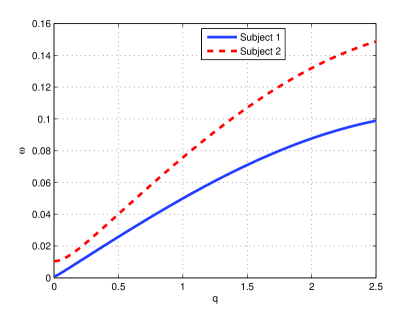
Figure 1: (Color online) The dispersion relation of the hormonal wave. Parameter values are: $D=0.12$ and $\Omega_{0}^{2}=a_{1}b_{2}$. Subject 1: $a_{1}=0.0226$, $b_{2}=0.0437$. Subject 2: $a_{1}=0.0509$, $b_{2}=0.2062$.

obtained by linearizing Eq.(8). As we observe in Fig. (1), the corresponding linear spectrum for the first two subjects of Ref. [19] is related to the system parameters. However for the parameter values related to the subject 2, the spectrum is increasing compared to the linear spectrum given by the parameter values related to subject 1.

Using the new scales $\xi_{n}=Z_{n}-V_{g}T_{n}$ and $\tau_{n}=T_{n}$, with velocity

$$V_{g}=\frac{D_{0}\sin(q)}{\omega},$$ (15)

we finally obtain the complex Ginzburg-Landau equation

$$i\frac{{\partial F_{1}}}{{\partial{\tau_{2}}}}+P\frac{{{\partial^{2}}F_{1}}}{{\partial\xi_{1}^{2}}}+(Q_{1}+iQ_{2}){\left|F_{1}\right|^{2}}F_{1}+i\gamma F_{1}=0,$$ (16)

where

$$\begin{split}&P=\frac{\omega^{2}D_{0}\cos(q)-D_{0}^{2}\sin^{2}(q)}{4\omega^{3}},\\ &Q_{1}=\frac{1}{\omega}\Big{[}\frac{2\lambda_{1}D_{2}\sin^{2}(\frac{q}{2})+\lambda_{1}^{2}}{\Omega_{0}^{2}}+\frac{\omega^{2}\nu_{1}^{2}-3\lambda_{1}^{2}+8\lambda_{1}^{2}\sin^{2}(\frac{q}{2})}{12\Omega_{0}^{2}+64D_{0}\sin^{4}(\frac{q}{2})}\Big{]},\\ &Q_{2}=\frac{-\lambda_{1}\nu_{1}}{2\Omega_{0}^{2}}+\frac{3\lambda_{1}\nu_{1}-4D_{2}\nu_{1}\sin^{2}(\frac{q}{2})}{12\Omega_{0}^{2}+64D_{0}\sin^{4}(\frac{q}{2})},\\ &\gamma=\frac{\nu_{0}}{4}+D_{1}\sin^{2}(\frac{q}{2}).\end{split}$$ (17)

During the last three decades, the CGL equation and its modified versions have drawn tremendous attention. These equations describe a variety of physical phenomena in optical waveguides and fibers, plasmas, Boose Einstein condensation, phase transitions, open flow motions, bimolecular dynamics, spatially extended non equilibrium systems, etc [23]. In the present research work, the CGL equation is an equation describing the evolution of modulated hormonal waves in a diffusive coupled pancreatic islet $\beta$-cells model. This result suggests that, the insulin propagates within the islet $\beta$-cells using both time and space domains in order to regulate glucose level. In another regard, oscillations of insulin secretion which are likely caused by intrinsic $\beta$-cell mechanisms generate a spatiotemporal dynamics of insulin between cells as modified by exogenous signals such as hormonal and neuronal input.

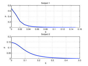
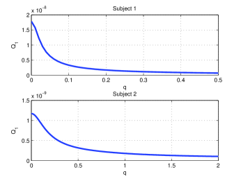
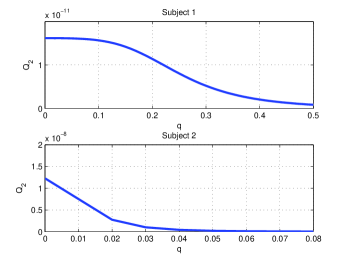
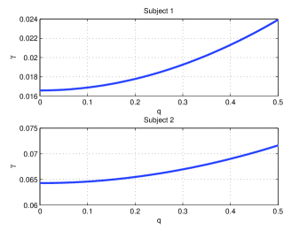
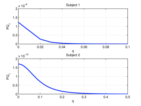
(a) (b) (c) (d) (e)

Figure 2: (Color online) Variations of coefficients (a) $P$, (b) $Q_{1}$, (c) $Q_{2}$, (d) the product $PQ_{1}$ as a function of the wave vector $q$ of the carrier wave. The parameter values are given in Table 1. Subject 1: $a_{1}=0.0226$, $a_{2}=3.8\times 10^{-8}$, $b_{1}=0.0022$, $b_{2}=0.0437$. Subject 2: $a_{1}=0.0509$, $a_{2}=1.29\times 10^{-7}$, $b_{1}=0.0096$, $b_{2}=0.2062$. With $D=0.12$.

We have represented in Fig. 2. the variations of constants $P$, $Q_{1}$, $Q_{2}$, $\gamma$ and of the product $PQ_{1}$ with respect to the wave vector $q$. The parameter values are those in the Table 1. It is observed for both subjects that the coefficients are positive for small values of the wave vector $q$. The nonlinearity coefficients have very small values. It is observed also that except the dissipative coefficient $\gamma$, all the other coefficients decrease with the increasing of the wave vector. It is well known that the complex Ginzburg-Landau equation has as the modulational instability criterion for the plane waves $P_{1}Q_{1}+P_{2}Q_{2}>0$ ($P_{1}$ and $P_{2}$ are the real and the imaginary parts of the dispersion coefficient, respectively) for which the plane waves in the system are unstable. This relation is known as the Lange and Newell’s criterion [24]. However, in this work the imaginary part of the dispersion coefficient is equal to zero, then the Lange and Newell’s criterion reduces to $P_{1}Q_{1}>0$ known as the Benjamin-Feir instability criterion [25]. According to this instability criterion, for $PQ_{1}>0$ wave planes in the system are unstable while for $PQ_{1}<0$, they are stable. Since the manner with which hormonal waves propagate in the system does not depend of the stability criterion, one can expect to find in the system spatiotemporal modulated wave solutions for any wave carrier whose wave vector is in the positive range of $PQ_{1}$.

3.2 Nonlinear solution of the equation of motion

The solutions of nonlinear partial differential equations constitute a crucial factor in the progress of nonlinear dynamics and are a key access for the understanding of various biological phenomena. Many analytical investigations have been carried out to find the envelope soliton solutions of these equations which are localized waves with particle like behavior i.e., preserving their forms in space or in time or both in space and time resulting in spatial, temporal or spatiotemporal solitons, respectively [26]. We assume that the form of the envelope soliton solution of Eq. (16) has the form of the one proposed by Pereira and Stenflo [14], and Nozaki and Bekki [15]

$$F_{1}(\xi_{1},\tau_{2})=\frac{Ae^{\phi}}{1+e^{(\phi+\phi^{*})^{(1+i\mu)}}}.$$ (18)

The real part $F_{1r}$ and the imaginary part $F_{1i}$ of $F_{1}(\xi_{1},\tau_{2})$ are given respectively by

$$F_{1r}(\xi_{1},\tau_{2})=A\Big{[}\frac{e^{-\phi}+\cos(2\mu\phi)e^{\phi}}{2(\cosh(2\phi)+\cos(2\mu\phi))}\Big{]}\,\,\,\,\,\mathrm{and}\,\,\,\,\ F_{1i}(\xi_{1},\tau_{2})=-A\Big{[}\frac{\sin(2\mu\phi)e^{\phi}}{2(\cosh(2\phi)+\cos(2\mu\phi))}\Big{]},$$ (19)

where $\phi=q\xi_{1}-\omega\tau_{2}$, $\mu=-\beta\pm\sqrt{2+\beta^{2}}$ and $\beta=-\frac{3Q_{1}}{2Q_{2}}$.

Using the solution of $F_{1}$ given by Eq. (19) and from Eq. (4), we have

$$y=2\epsilon(F_{1r}\cos\theta-F_{1i}\sin\theta)+\epsilon^{2}[F_{0}+2(F_{2r}\cos 2\theta-F_{2i}\sin 2\theta)]+O(\epsilon^{3}),$$ (20)

where $F_{2r}$ and $F_{2i}$ are the real and imaginary parts of $F_{2}$, respectively such that

$$F_{2r}=c_{1}(F_{1r}^{2}-F_{1i}^{2})+2c_{2}F_{1r}F_{1i}\,\,\,\,\,\mathrm{and}\,\,\,\,\,F_{2i}=c_{2}(F_{1i}^{2}-F_{1r}^{2})+2c_{1}F_{1r}F_{1i},$$ (21)

with

$$c_{1}=\frac{\lambda_{1}-4D_{2}\sin^{2}(\frac{q}{2})}{3\Omega_{0}^{2}+16D_{0}\sin^{4}(\frac{q}{2})}\,\,\,\,\,\mathrm{and}\,\,\,\,\,c_{2}=\frac{\omega\nu_{1}}{3\Omega_{0}^{2}+16D_{0}\sin^{4}(\frac{q}{2})}.$$ (22)

Inserting Eqs. (19) and (21) into Eq. (20), we obtain for the insulin dynamics the following solution

$$\begin{split}y_{n}(t)=&\epsilon A\Big{[}\frac{\cos(\theta_{n}-2\alpha\phi_{n})e^{\phi_{n}}+\cos\theta_{n}e^{-\phi_{n}}}{(\cosh 2\phi_{n}+\cos 2\alpha\phi_{n})}\Big{]}+\epsilon A^{2}\Big{[}-\frac{\lambda_{1}}{\Omega_{0}^{2}(\cosh 2\phi_{n}+\cos 2\alpha\phi_{n})}\Big{]}\\ &+\epsilon^{2}A^{2}\Big{[}(c_{1}\cos 2\theta_{n}+c_{2}\sin 2\theta_{n})\times\Big{(}\frac{2\cos 2\alpha\phi_{n}+\cos 4\alpha\phi_{n}e^{2\phi_{n}}+e^{-2\phi_{n}}}{(\cosh 2\phi_{n}+\cos 2\alpha\phi_{n})}\Big{)}\Big{]}\\ &+\epsilon A^{2}\Big{[}(c_{1}\sin 2\theta_{n}-c_{2}\cos 2\theta_{n})\times\Big{(}\frac{2\sin 2\alpha\phi_{n}+\sin 4\alpha\phi_{n}e^{2\phi_{n}}}{(\cosh 2\phi_{n}+\cos 2\alpha\phi_{n})}\Big{)}\Big{]},\end{split}$$ (23)

where $\phi_{n}=\epsilon q(n-V_{g}t)-\omega\epsilon^{2}t$.

In Fig. 3, we have represented the evolution of the solution at different times according to the parameter values related to the two first healthy subjects of Ref. [19]. As we observe in this figure, the solution is well a localized modulated solution, and its propagates structurally stable. As interestingly remarked in the present work, the modulated solution involving in the system appears in the form of a breather-like coherent structure and it propagates with the same dynamics for the different parameter values related to the two healthy subjects. This assumption can lead to the conclusion that the insulin propagates in pancreatic islet $\beta$-cells using localized modulated solitonic waves.

Let us recall that the localized modulated oscillations obtained in this work are involved in many other biophysical systems. Under certain conditions, they can move and transport energy along the system [27, 28, 29]. As recently demonstrated in [27], breathing modes are also responsible of energy sharing between $\alpha$-polypeptide coupled chains. Also, localized oscillations can be precursors of the bubbles that appear in thermal denaturation of DNA and they have been shown to describe the breaking of the hydrogen bonds linking two bases [28]. It has been also shown that these localized oscillations can move along microtubule systems [29]. Then, breathers should be understood as triggering signal for the motor proteins to start moving as interestingly find also in this work.

In Fig. 4, we have increased the value of $\epsilon$ from $\epsilon=0.077$ to $\epsilon=0.099$, with the same parameter values used in Fig. 3. It clearly reveals in this figure the influence of small perturbation in the dynamics of the hormonal wave. One can easily see that for both subjects the solutions still remain the breather excitations. However these breathers are now represented by modulated solitons so that the envelopes cover less oscillations of the carrier wave as those observed in Fig. 3. It is also observed that the amplitude of the wave has increased.

4 Conclusion

We have studied the intercellular insulin dynamics in an array of diffusively coupled pancreatic islet $\beta$-cells. The model was formulated by a system of discrete ordinary differential equations where the cells are connected via gap junction coupling. Motivated with often non-observance clinical effects due to some pathological diseases [10], the work was devoted to derive a clear analytical solution describing the insulin dynamics in pancreatic islet $\beta$-cells. Applying a powerful perturbation technique, we have found that the complex Ginzburg-Landau equation is the equation which describes the insulin dynamics. It has been revealed that the solution of the hormonal wave is well a localized modulated solitonic wave called breather. In another regard, the breather has been revealed as mechanically important in other biophysical systems such as collagen [27], DNA [28], microtubule [29] systems. The correlation with the present work may indicate an important role of breathers and other nonlinear excitations in the dynamics of pancreatic islet $\beta$-cells. In a forthcoming work, we intend to investigate long-range effect, since intercellular waves travel also with non contacting cells [31, 32] indicating the long-range interaction in the system.

References

F.M. Ashcroft, J. Clin. Invest. 115, 2047 (2005).

B.E. Isackson, W.H. Evans, S. Boitano, Am. J. Physiol. 280, L221 (2001).

Y. Osipchuk, M. Cahulan, Nature 359, 241 (1992).

A.M. Hofer, S. Curci, M.A. Doble, E. M. Brown, D.I. Soybel, Nat. Cell Bio. 2, 392 (2000).

M.E. Gracheva, J.D. Gunton, J. Theor. Biol. 221, 513 (2003).

P. Gilon, M. A. Ravier, J.C. Jonas, J. C. Henquin, Diabetes 51, S144 (2002).

J. Sneyd, M. Wilkins, A. Stahonja, M. Sanderson, Biophys. Chem. 72, 101 (1998).

The diabetes Control and Complications Trial Research, New England J. Med. 329, 977 (1993).

A. De Gaetano, G. Mingrone, M. Castagneto, P.A. Tataranni, A.V. Greco, Am. J. Physiol. 271, E93 (1996)

R.A. Defronzo, E. Ferrannini, Diabetes Care 14, 173 (1991)

S. Frontoni, L. Ohman, J.R. Haywood, R.A. Defronzo, L. Rossetti, Am. J. Physiol. 262, E191 (1992).

N.R. Pereira, L. Stenflo, Phys. Fluids 20, 1733 (1977).

K. Nozaki, N. Bekki, J. Phys. Soc. Jpn. 53, 1581 (1984).

S. Raghavachari, J.A. Glazier, Phys. Rev. Lett. 82, 2991 (1999).

M. Perez-Armandriz, M.C. Roy, D.C. Spray, M.V.L. Bennet, Biophys. J. 59, 76 (1991).

J.P. Keener, Bull. Math. Bio. 63, 625 (2001).

A. De Gaetano, O. Arimo, J. Math. Biol. 40, 136 (2000).

M. Remoissenet, Phys. Rev. B. 33, 2386 (1986).

D.J. Kaup, A.C. Newell, Phys. Rev. B 1S, 5162 (1978).

A.C. Newell, J. Math. Phys. 19, 1126 (1978).

A. Hasegawa, Plasma Instabilities and Nonlinear Effects (Springer Verlag, Berlin, 1975).

C.G. Lange and A.C. Newell: SIAM J. Appl. Math. 27, 441 (1974).

T.B. Benjamin and J.E. Feir: J. Fluid Mech. 27, 417 (1967).

S. Shwetanshumala, Progress In Electromagnetics Research Letters 3, 17 (2008).

A. Mvogo, G.H. Ben-Bolie, T.C. Kofane, Chaos 25, 063115 (2015).

T. Dauxois, M. Peyrard, A.R. Bishop, Phys. Rev. E 47, R44 (1993).

S. Zdravkovi, A.N. Bugay, G.F. Aru, A. Maluckov, Chaos 24, 023139 (2014).

G.D. Mitsis, M.G. Markakis, V.Z. Marmarelis, IEEE, Trans. Biomed. Eng. 56, 2347 (2009).

A. Mvogo, A. Tambue, G. H. Ben-Bolie, T.C. Kofane, Commun Nonlinear Sci Numer Simulat 39, 396 (2016).

W.D. Kepseu, P. Woafo, Phys. Rev. E 78, 011922 (2008).

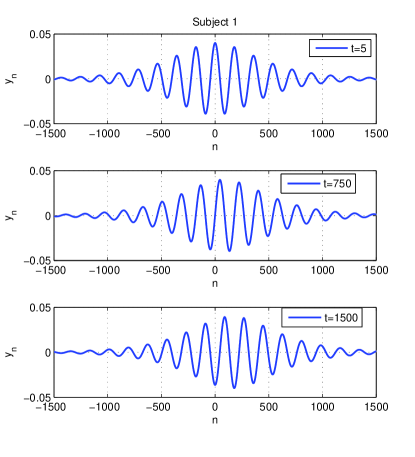
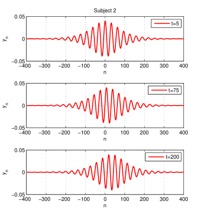
(a) (b)

Figure 3: (Color online) The solution $y_{n}$ as a function of the position at different times. The parameter values are: Subject 1: $D=0.12$, $q=0.035$, $\epsilon=0.077$, $a_{1}=0.0226$, $b_{1}=0.0022$, $a_{2}=3.8\times 10^{-8}$, $b_{2}=0.0437$. Subject 2: $D=0.12$, $q=0.2$, $\epsilon=0.077$, $a_{1}=0.0509$, $a_{2}=1.29\times 10^{-7}$, $b_{1}=0.0096$, $b_{2}=0.2062$.

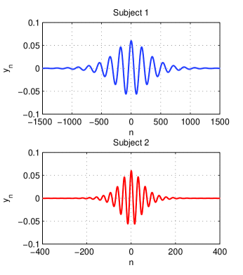
Figure 4: (Color online) Effects of small perturbation on the hormonal modulated wave. $\epsilon=0.099$ and $t=5$. The parameter values are the same as in Fig.3.