Direct determination of oxygen abundances in line emitting star-forming galaxies at intermediate redshift.

Abstract

We present a sample of 22 blue ($(B-V)_{AB}<0.45$), luminous ($M_{B,AB}<-18.9$), metal-poor galaxies in the $0.69<z<0.88$ redshift range, selected from the DEEP2 galaxy redshift survey. Their spectra contain the [OIII] $\lambda 4363$ auroral line, the [OII]$\lambda\lambda 3726,3729$ doublet and the strong nebular [OIII]$\lambda\lambda 4959,5007$ emission lines. The ionised gas-phase oxygen abundances of these galaxies lie between $7.62<12+\log O/H<8.19$, i.e. between $1/10Z_{\odot}$ and $1/3Z_{\odot}$. We find that galaxies in our sample have comparable metallicities to other intermediate-redshift samples, but are more metal poor than local systems of similar B-band luminosities and star formation activity. The galaxies here show similar properties to the “green peas” discovered at $z\simeq 0.2-0.3$ though our galaxies tend to be slightly less luminous.

1 Introduction

The study of metal poor, compact star forming galaxies was initiated by Searle & Sargent (1972). Their importance was rapidly recognized because they were considered to be ideal benchmarks in the study of the earliest stages of galaxy evolution, and were studied in many works (Campbell (1988); Pagel et al. (1992); French (1980), among many others). While these nearby systems were originally thought to be genuinely young systems, experiencing their very first star forming episodes, even the most metal poor objects in the local universe have been found to posses significant underlying evolved stellar populations, e.g., (Papaderos et al., 1996; Taylor et al., 1995). In fact, very deep Hubble Space Telescope images of the most metal-poor object known, I Zw 18, indicate that it has formed the bulk of its present stellar population 0.5–1.0 Gyr ago (Aloisi, Tosi, & Greggio, 1999). Other works on the stellar populations of this and similar galaxies yield similar results (Papaderos et al., 2002; Aloisi et al., 2007). A motivation to examine samples at higher redshifts is to locate truly young systems that could be experiencing their first major star formation episodes. Some exploratory steps in this direction were taken by Hoyos et al. (2005), who found that distant ($z\sim 0.7$), compact star forming galaxies showing the [OIII]$\lambda$4363 line deviated from the usual Luminosity-Metallicity relationships, implying that these distant, metal poor systems might turn out to be truly young systems. One of the aims of this paper is to further explore this hypothesis.

Knowledge of the metallicity of external galaxies is crucial for galaxy evolution theories because it is a direct result of the integral history of the star formation and mass assembly of galaxies. The metallicity of galaxies has been traditionally used in conjunction with the luminosity to build the luminosity-metallicity relation (LZR) see, e.g., Lequeux et al. (1979); Richer & McCall (1995). This relationship is thought to arise from depth of the gravitational well of massive galaxies which does not allow newly created metals being cast into the ISM amidst hot supernovae ejecta, where it is assumed that the more luminous galaxies are also the most massive, and have a higher star formation efficiency. In this model, lower mass systems will not be able to keep their heavy elements and will probably be of lower metallicity. Galaxies in cluster environments undergo other processes, which greatly complicate the picture. All these phenomena will naturally create a complex metallicity distribution for galaxies at various redshifts, of which only a few data points at intermediate redshifts are precisely known.

This paper addresses the star formation history of galaxies by examining the properties of a sample of star forming galaxies showing the [OIII]$\lambda 4363$ line.

The [OIII]$\lambda$4363 auroral line is generated by the collisionally excited transition (2p²¹D to 2p²¹S) of doubly ionised oxygen atoms. This line is key in the study of the metallicity of the ionised phase of the interstellar medium (ISM) since it allows determining the electron temperature of ionised regions without any previous assumption on the metal content of the observed nebula (Osterbrock & Ferland, 2006). Unfortunately, the [OIII]$\lambda$4363 line is difficult to detect for several reasons: (i) This line is stronger in low metallicity clouds. In higher metallicity environments, it is exponentially depressed because the increased cooling leaves no energy to excite oxygen atoms to the upper level of this transition. (ii) This line is also stronger in young and strong starbursts. Older starbursts (older than 5–6 Myr) are unable to maintain a large fraction of oxygen atoms doubly ionised. (iii) This line is also stronger in systems in which the contribution to the continuum from the underlying stellar population is less important relative to the contribution from the newly created ionising stars. The latter case is the one where this weak line is less likely to be obliterated by the continuum noise. In Hoyos & Díaz (2006), it was shown that all these issues affect the detection of the [OIII]$\lambda$4363 Å line for the case of local HII galaxies.

The discussion above explains why the majority of the most accurate metallicity determinations for intermediate redshift sources have been obtained using measurements of the auroral oxygen lines in galaxies with strong starbursts. At the same time, it also explains why these measurements may not be fully tracing the complete metallicity distribution at each redshift, since the upper end of this distribution is increasingly difficult to trace accurately through the use of the oxygen lines. Furthermore, even in the $12+\log O/H\sim 8.10-8.35$ regime, the oxygen-based strong line calibrators such as $\mathrm{R}_{23}$ allow two solutions, a problem difficult to overcome. An alternative is to use [SIII]$\lambda\lambda 9096,9532$, suggested for instance by Pérez-Montero et al. (2006), which does not exhibit the degeneracies that $\mathrm{R}_{23}$ has at intermediate metallicities. Finally, it is also possible to determine electron temperatures through the detection of [SIII]$\lambda 6312$ line up to at least solar metallicities and then derive good abundances for high-metallicity, vigorously star forming systems. This has been shown in Kinkel & Rosa (1994), Bresolin et al. (2005), Díaz et al. (2000), and Castellanos, Díaz, & Terlevich (2002). One disadvantage in the use of sulfur lines is that they shift into the NIR for objects at even moderate redshifts. However, the work of An et al. (2013) shows that this is being addressed with new IR instrumentation. The latter work presents a study on the nature of the [SIII]$\lambda\lambda 9096,9532$ emitters, showing that these objects are usually star forming systems where a Compton-thick AGN has little or no effect in exciting the sulfur lines.

The work presented in Hoyos et al. (2005) also investigated the differences between star forming systems with and without the [OIII]$\lambda$4363 Å line using intermediate redshift ($z\simeq 0.7$) galaxies observed by the DEEP2 survey. Compact, star forming galaxies showing the [OIII]$\lambda 4363$ auroral line have lower metallicities and higher emission line equivalent widths than objects without this feature, in spite of their H$\beta$ line luminosities not being lower. This was also found by Hoyos & Díaz (2006). The underlying stellar populations of galaxies presenting the [OIII]$\lambda$4363 are less luminous relative to their newly created ionising populations, when compared to other star forming galaxies (Hoyos & Díaz, 2006).

In this paper, §2 describes the observations and sample selection, §3 shows our metallicity calculations based on electron temperatures.We compare our results to other recent works dealing with both local and intermediate redshift sources in §4. This section also summarizes the paper. We use $(\Omega_{M},\Omega_{\Lambda},h_{70})=(0.3,0.7,1)$. Magnitudes are given in the $AB$ system.

2 Observations and Sample Selection.

The data used in this work were taken for the second phase of the Deep Extragalactic Evolutionary Probe survey (DEEP2, Newman et al. (2013)). This survey uses the DEIMOS (Faber et al., 2003) spectrograph on the W.M. Keck telescope. DEEP2 is a densely sampled, high precision redshift survey which, thanks to a $BRI$ colour pre-selection criterion, preferentially targets galaxies in the $0.7<z<1.4$ redshift range in three of the four areas of the sky it covers. It has collected a grand total of 53000 spectra, measuring 38000 reliable redshifts. The DEIMOS instrument was used with a 1200$\mathrm{mm}^{-1}$ grating centered at 7800Å, thus covering on average the 6500Å-9100Å wavelength range. The wavelength range shows slight changes that depend on the slit position on the mask. The resolving power ($R\simeq 5000$) allows separating the [OII]$\lambda\lambda 3726,3729$ doublet. Because of the relatively high resolution, the DEEP2 spectra also yield accurate velocity dispersions for emission line objects.

We select galaxies showing the strong oxygen emission lines [OII]$\lambda 3727$, [OIII]$\lambda 4959$ and that have a reliable detection of the weak auroral line [OIII]$\lambda 4363$ in their spectra. There is no need to include the [OIII]$\lambda 5007$ in the selection criteria since its intrinsic emission is linked to that of the [OIII]$\lambda 4959$ line and its reddening-corrected flux can be found as $I_{5007}=2.98\times I_{4959}$ for normal star forming systems. The combination of these requirements limit the redshift range to $0.69<z<0.88$, which includes $\sim 11000$ potential candidates. This initial culling was made possible by the Weiner, B. J. priv. comm. redshifts and equivalent width measurements. The remaining spectra were visually inspected for reliable detections of the auroral [OIII]$\lambda 4363$ line, and to ensure the [OII]$\lambda 3727$ doublet is cleanly separated. This allows measuring the electron density accurately, without any previous assumptions. We measured the emission line parameters measured using the IRAF tasks ngaussfit and splot. Our final sample consists of 22 sources, or about 0.2% of the potential candidates in the relevant redshift window. Figure 1 shows two example spectra of the final sample.

Figure 1: Rest frame spectra of two metal-poor galaxies - DEEP2_130016475 at $z=0.747$ (left panel) and DEEP2_31046514 at $z=0.789$ (right panel). Both show the temperature sensitive [OIII]$\lambda 4363$ line used to select the sample and the other oxygen emission lines used to measure the ionic and total abundances. Because of the slit location on the mask, the spectrum in the left panel is cutoff at a rest-wavelength blueward of [OIII]$\lambda 5007$.

The number count $S/N$ ratio of the $H{\gamma}$ line is in the $15<S/N_{\gamma}<100$ interval with a typical value of $S/N_{\gamma}=50-60$. In the case of the [OIII]$\lambda 4363$, we have $4.1<S/N_{4363}\leq 11.5$ with an average value of $S/N_{4363}=10.0$. We thus have a worst-case uncertainty in the [OIII]$\lambda 4363/\mathrm{H}\gamma$ of 25%, with a typical value of 10%. The relative error in the [OIII]$\lambda 4363/\mathrm{H}\gamma$ ratio is a major contributor to the error in the electron temperatures and therefore oxygen abundances in the direct method we use to derive metallicities. However, in this analysis, the determination of the electron temperatures are robust relative to these uncertainties.

We stress here that, because of our visual sample selection, the galaxies used here do not define a complete set in statistical terms. However, they are representative of the intermediate redshift population of emission line galaxies with good metallicity determinations that show [OIII]$\lambda 4363$.

The DEEP2 parent sample was selected from photometry obtained at the Canada-France-Hawaii Telescope (CFHT) in the $B$, $R$ and $I$ bands using the CFHT 12k$\times$8k camera (Coil et al., 2004). The catalogues were generated using the imcat software (Kaiser, Squires, & Broadhurst, 1995) and the object magnitudes in $R$ are measured within a circular aperture with a radius of 3 $r_{g}$ where $r_{g}$ is the optimal Gaussian profile unless 3 $r_{g}$ were less than 1$"$ , in which case the flux is measured inside a 1^′′ aperture. The $B-R$ and $R-I$ colours are measured with apertures of 1^′′ in order to minimise the noise (Coil et al., 2004). The rest-frame magnitudes were obtained following Willmer et al. (2006) and use as templates a set of 34 local galaxies observed by Kinney et al. (1996). For each galaxy a parabolic fit between the synthetic $B-R$ and $R-I$ colours and $U-B$ measured at the galaxy redshift is used to estimate the rest-frame B magnitude and $U-B$ colour. The rms errors for the K-corrections are usually smaller than 0.15 magnitudes measured at the high redshift edge of DEEP2 ($z\sim 1.5$). The rms errors for the $U-B$ colours range from 0.12 mag at $z=1.2$ (worst value) to 0.03 mag at redshifts where the observed filters best overlap $U-B$ (Willmer et al., 2006). For more detailed descriptions of both procedures we refer the reader to Coil et al. (2004) and Willmer et al. (2006).

Table 1 summarises the selected sample, where we present the object identification from the DEEP2 catalogue, coordinates on the sky, observed and rest-frame magnitudes, the rest-frame equivalent width of H$\beta$ and the velocity dispersions. The rest-frame colours are consistent with these sources containing vigorous star forming clusters. The measured velocity dispersions indicate that none of the sources hosts Active Galactic Nucleus (AGN) activity, as defined by the criterion presented in Osterbrock & Ferland (2006), which sets the limit between AGNs and normal star forming systems at around $180\mathrm{km}\mathrm{s}^{-1}$.

Table 1: Full DEEP2 IDs, redshifts, J2000 coordinates, AB apparent and absolute B-band magnitudes, AB $UBV$ colours, $H\beta$ rest frame equivalent width and velocity dispersion. Uncertainties in EW(H$\beta$) are a few Å.

ID	$z$	RA	DEC	$m_{B}$	$M_{B}$	$U-B$	$B-V$	EW(H$\beta$)	$\sigma$
		$(hh:mm:ss)$	$(dd:mm:ss)$	$(mag_{ob})$	$(mag)$	$(mag)$	$(mag)$	${(\AA)}$	(km/s)
21007232	0.71659	16:47:26.19	02:19:00.81	23.40	-20.04	0.47	0.35	36	37$\pm$2
41022570	0.72138	02:27:30.46	00:02:04.43	23.43	-19.47	0.39	0.31	310	29$\pm$2
42009827	0.72939	02:29:33.65	00:01:44.53	23.97	-19.32	0.36	0.25	80	30$\pm$2
42025672	0.73143	02:29:02.03	00:02:00.54	22.87	-20.07	0.36	0.28	122	48$\pm$3
31047738	0.73232	23:26:41.18	00:01:13.06	22.60	-20.53	0.33	0.23	93	38$\pm$3
22006008	0.73280	16:51:08.82	02:19:04.23	24.52	-18.92	0.44	0.32	13	25$\pm$5
22032374	0.73839	16:53:06.12	02:19:57.79	23.60	-19.94	0.51	0.38	38	35$\pm$2
32018903	0.73961	23:30:55.46	00:00:47.86	23.73	-19.65	0.48	0.36	89	46$\pm$7
13016475	0.74684	14:20:57.85	52:56:41.81	22.97	-20.16	0.49	0.38	162	47$\pm$6
22032252	0.74872	16:53:03.49	34:58:48.95	24.21	-19.30	0.49	0.36	78	37$\pm$3
31019555	0.75523	23:27:20.37	00:05:54.76	23.56	-19.27	0.53	0.43	165	52$\pm$2
14018918	0.77091	14:21:45.41	53:23:52.70	23.14	-20.23	0.44	0.32	124	42$\pm$2
12012181	0.77166	14:17:54.62	52:30:58.42	23.37	-19.77	0.37	0.27	42	41$\pm$3
41059446	0.77439	02:26:21.48	00:48:06.81	22.68	-20.92	0.35	0.24	35	45$\pm$3
41006773	0.78384	02:27:48.87	00:24:40.08	23.97	-19.27	0.33	0.23	36	30$\pm$2
31046514	0.78856	23:27:07.50	00:17:41.50	23.84	-20.11	0.46	0.33	47	48$\pm$2
22020856	0.79448	16:51:31.47	34:53:15.96	23.50	-20.13	0.45	0.32	68	42$\pm$4
22020749	0.79679	16:51:35.22	34:53:39.48	23.53	-20.16	0.42	0.30	102	49$\pm$4
22021909	0.79799	16:50:55.34	34:53:29.88	24.06	-19.35	0.24	0.16	25	32$\pm$7
21027858	0.84107	16:46:29.01	02:19:41.33	23.56	-20.14	0.29	0.20	93	56$\pm$1
22022835	0.84223	16:50:34.61	02:19:31.49	23.47	-19.85	0.32	0.23	250	50$\pm$4
31047144	0.85623	23:26:55.43	00:01:11.53	23.33	-20.27	0.25	0.18	87	55$\pm$2

In Figure 2, we compare our selected sample against other DEEP2 sources in the same redshift interval. The comparison galaxies were selected according to their $\mathrm{H}\beta$ line equivalent widths. The purpose of this comparison is to highlight the nature of the [OIII]$\lambda 4363$ galaxies, showing that their star formation episodes are both very intense and young. The first comparison sample contains 4550 galaxies with $\mathrm{EW}_{\beta}>10\mathrm{\AA}$, which represents the general population of DEEP2 emission-line galaxies at these redshifts. The second one contains 218 galaxies with $\mathrm{EW}_{\beta}>50\mathrm{\AA}$, which represents either galaxies with an AGN or systems with very young and vigorous star forming episodes. It is seen that the [OIII]$\lambda 4363$ galaxies are very blue and luminous. Some of the galaxies selected for this work are actually amongst the bluest DEEP2 targets, even in the $U-B$ colour, hinting that our spectroscopically selected sample must be comprised of galaxies with very intense starbursts.

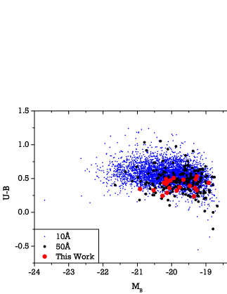
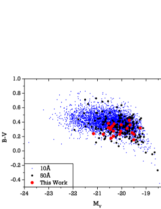
Figure 2: $U-B$ vs. $B$ and $B-V$ vs. $V$ CMDs. The blue dots depict 4550 objects with $\mathrm{EW}(H\beta)\geq 10\mbox{\AA}$. The black dots show the 218 galaxies with $\mathrm{EW}H\beta)\geq 50\mbox{\AA}$. Our sample is presented as large red solid circles.

3 Results

3.1 Relative flux calibration. Special case for the [OII]$\lambda 3727$ doublet.

The DEEP2 spectra are not flux calibrated so that it is necessary to make a relative flux calibration for each spectrum in order to obtain the physical line ratios. Here, we use the results provided by Konidaris (2008), who fits a smooth fourth order polynomial to model the relative throughput with wavelength. This allows measuring meaningful observational line ratios, without the need to perform a full flux-calibration of the spectra. In our procedure, we first normalize the observed number counts of any given oxygen line to the number counts of its nearest hydrogen Balmer line, obtaining an instrumental line ratio. Therefore, we first compute $F(\mathrm{[OIII]}\lambda,\lambda 4959,5007)/F(\mathrm{H}\beta)$ and $F(\mathrm{[OIII]}\lambda 4363)/F(\mathrm{H}\gamma)$ in instrumental units and then apply the relative calibration explained in Konidaris (2008), for which a brief summary is presented as an appendix. In cases where two lines are close in wavelength space, there is no need to apply the throughput correction, since the latter is almost identical for both the numerator and denominator in the two expressions. However, for the [OII]$\lambda 3727$ doublet the Konidaris (2008) calibration is used as there are no H series lines close enough in wavelength, as the case of the [OIII] lines. In this case the relative flux calibration uses the $F(\mathrm{[OII]}\lambda 3727)/F(\mathrm{H}\gamma)$ ratio. The typical uncertainty in the empirical Konidaris (2008) calibration is of the order of 10%, which must be propagated into the aforementioned ratio. This is a major contributor to the error budget in this specific line ratio, together with the uncertainty in fixing the [OII]$\lambda 3727$ continuum level for vigorously star forming objects. An additional source of error is related to the possible presence of an underlying stellar population contributing to the continuum, although most of the objects studied here do not show strong absorption wings in the Balmer lines. Typical values of the absorption $H\beta$ equivalent width found for line-emiting star forming galaxies are in the range 0–3.5 Å for a spectral resolution of about 7 Å (Izotov et al., 1994) . For the higher spectral resolution of the data analysed here ($R\sim 5000$, at 7800Å ) these contributions are considerably reduced, involving only the core of the line (Diaz, 1988). If we adopt a rest frame $\mathrm{H}\beta$ absorption equivalent width of the order of 1Å , the underlying absorption correction is typically small, about 2% in H$\beta$ and 3% in H$\gamma$ due to the large Balmer emission equivalent widths. However, given that we are measuring electron temperatures via equation 1 below, the impact of this uncertainty in our determination of the electron temperature affects the $R_{O3}$ ratio defined below at the 1% level at most.

3.2 Temperatures, densities, and oxygen content calculations.

Given the expected physical conditions of the line emitting regions in the galaxies of this sample, it is safe to assume that all oxygen is either singly or doubly ionised. The $O^{+}/O^{0}$ ratio is fixed to the $H^{+}/H^{0}$ ratio via a charge exchange reaction, and is almost surely negligible in this case. It would also require exceptionally hard radiation in order to produce a significant amount of $O^{3+}$. Therefore, we use a two phase model with a low ionisation zone which depends on the emission of the [OII]$\lambda 3727$ doublet, and a high ionisation zone in which the OIII lines are formed.

Table 2 summarises the required line ratios to solve the two-phase scenario, assuming the electron density of the higher ionization zone to be equal to the electron density in the lower ionization zone. At any rate, the electron densities found are well below the critical value for de-excitation. From our observations, we can obtain $R_{O3}$ and $R_{ne}$. It is, however, not possible to calculate $R_{O2}$ as we cannot measure the auroral [OII] lines as their observed wavelengths for this sample of galaxies fall beyond the coverage of DEIMOS.

Table 2: Line ratios used to derive electron densities and temperatures. $I(nnnn)$ is the reddening-corrected intensity of each emission line.

Quantity.	Diagnostic.
$t_{e}$[OIII]	$R_{O3}=(I(4959)+I(5007))/I(4363)$
$t_{e}$[OII]	$R_{O2}=I(3727)/(I(7319)+I(7330))$
$n_{e}$[OII]	$R_{ne}=I(3726)/I(3729)$

We measure the physical ratio via the closest H line using the normalised flux measurements defined in §3.1 and simultaneously account for internal extinction, assuming the theoretical case B recombination value for Balmer decrements I(H$\gamma$)/I(H$\beta$)=0.471, which is the mean between the values corresponding to $T_{e}=10000K$ and $T_{e}=20000K$ for $n_{e}=100\mathrm{cm}^{-3}$, as is seen in Osterbrock & Ferland (2006).

$$R_{O3}=\frac{[f(4959)+f(5007)]/f(H\beta)}{f(4363)/f(H\gamma)}\frac{I(H\beta)}{I(H\gamma)}$$ (1)

where, in this case, $f(nnnn)$ represents the observed number counts of each emission line.

This expression is used because the $R_{O3}$ ratio involves lines with different wavelengths and therefore we need to minimise errors arising from the relative flux calibration. This is accomplished by measuring the line number counts in units of the nearest Balmer line.

On the other hand, the ratio between the two lines in the [OII]$\lambda 3727$ doublet $R_{ne}$ bears the lowest uncertainty, as it is not affected by flux calibration or reddening issues. The error in our electron density determinations is thus dominated by the uncertainty in the electron temperature of the O⁺ zone.

We have derived the physical conditions of the $O^{++}$ dominated region using the expressions given by Hägele et al. (2008) for the oxygen emission lines of HII galaxies. This formula is an approximation for the statistical equilibrium model in a five level atom. We present below the adequate fitting function they used from the temden task of iraf, which is based on the program fivel (De Robertis, Dufour, & Hunt (1987) and Shaw & Dufour (1995)):

$$t_{e}\mbox{[OIII]}=0.8254-0.0002415\times R_{O3}+\frac{47.77}{R_{O3}}.$$ (2)

The expected deviations in electron temperatures that could arise from the use of this expression are 5% or lower. In our case, the electron temperatures in the $O^{+}$ ionisation zone needs to be estimated from $t_{e}\mathrm{[\textsc{OIII}]}$ because the [OII] auroral lines are not included in the spectral range covered by the DEIMOS spectra. Thus, the empirical expression given in Pagel et al. (1992), which is based on a fit to the theoretical models first presented in Stasińska (1990) is used:

$$t_{e}^{-1}\mbox{[{OII}]}=0.5(t_{e}^{-1}\mbox{[{OIII}]}+0.8)$$ (3)

The uncertainties in $t_{e}\mathrm{[\textsc{OII}]}$ are therefore a convolution between the $t_{e}\mathrm{[\textsc{OIII}]}$ errors and the variety of models used to derive the above expression for the electron temperature in the $O^{+}$ zone. These errors are bound to be higher than the errors for $t_{e}\mathrm{[\textsc{OIII}]}$, and are estimated to be about 40%. The errors quoted in Table 3 only reflect the standard error propagation from the Stasińska (1990) expressions and our $t_{e}\mathrm{[\textsc{OIII}]}$ uncertainties. Once the 40% intrinsic scatter of the $t_{e}\mathrm{[\textsc{OII}]}$ calibration is taken into account, this translates into a 50% error in the $O^{+}/H^{+}$ ionic abundance, or 0.3 dex. Because most of the oxygen in the ionised gas-phase will probably be in the form of $O^{2+}$, the large uncertainties for the $O^{+}$ content will not affect significantly the error budget for the final oxygen abundance. Table 3 shows the resulting electron temperatures and densities. It is seen that the electron density is close to the expected value of $100\mathrm{cm}^{-3}$. This is much lower than the critical density $n_{\mathrm{crit}}$ where the higher energy level of the observed lines are as likely to be de-excited by collisions as by radiative decay. This indicates that our $t_{e}\mathrm{[\textsc{OII}]}$ calculations are valid. For some galaxies, the resulting electron densities we obtain are smaller than $50\mathrm{cm}^{-3}$, and for these only upper limits are quoted. Using the results above and the expressions of Hägele et al. (2008) we calculate the partial ionic abundances $12+\log(O^{+}/H^{+})$ and $12+\log(O^{++}/H^{+})$. These are then combined to obtain the final oxygen abundance, where we assume the fractions of O⁰ and O³⁺ are negligible:

$$\frac{O}{H}=\left(\frac{O^{+}}{H^{+}}\right)+\left(\frac{O^{2+}}{H^{+}}\right)$$ (4)

Table 3 presents the resulting ionic and total abundances and the ratio between the two ionisation states $\log(O^{2+}/O^{+})$ in the gas. The errors are smaller than 0.1 dex for the oxygen ionic and total abundances and between 0.1 and 0.15 dex for the O²⁺/O⁺ ratio. The low oxygen abundances, corresponding to metallicities from 1/3 to 1/10 of the solar value, combined with the extreme colour-magnitude properties of the sample show that these galaxies are metal-poor.

Table 3: Results from nebular analysis. Abundances, electron densities and electron temperatures for the O2+ zone.

ID	$z$	$n_{e}$	$T_{e}(O^{2+})$	$12+\log(O^{+}/H^{+})$	$12+\log(O^{2+}/H^{+}$)	$12+\log(O/H)$	$\log(O^{2+}/O^{+})$
		$(cm^{-3})$	$(10^{4}K)$
21007232	0.71659	100	1.16$\pm$0.09	7.72$\pm$0.11	7.98$\pm$0.10	8.17$\pm$0.11	0.26$\pm$0.21
41022570	0.72138	230	1.34$\pm$0.03	7.35$\pm$0.06	7.84$\pm$0.03	7.96$\pm$0.04	0.50$\pm$0.09
42009827	0.72946	70	1.47$\pm$0.07	7.42$\pm$0.08	7.80$\pm$0.05	7.95$\pm$0.06	0.38$\pm$0.13
42025672	0.73152	$<50$	1.17$\pm$0.03	7.42$\pm$0.07	8.03$\pm$0.04	8.13$\pm$0.04	0.61$\pm$0.10
31047738	0.73239	110	1.13$\pm$0.04	7.73$\pm$0.07	8.00$\pm$0.04	8.19$\pm$0.05	0.27$\pm$0.12
22006008	0.73282	100	1.78$\pm$0.13	7.45$\pm$0.09	7.49$\pm$0.07	7.77$\pm$0.08	0.04$\pm$0.16
22032374	0.73839	$<50$	1.53$\pm$0.09	7.29$\pm$0.08	7.69$\pm$0.07	7.83$\pm$0.07	0.40$\pm$0.15
32018903	0.73956	65	1.38$\pm$0.06	7.42$\pm$0.08	7.89$\pm$0.05	8.02$\pm$0.06	0.47$\pm$0.13
13016475	0.74684	200	1.29$\pm$0.02	7.08$\pm$0.06	7.97$\pm$0.02	8.03$\pm$0.02	0.89$\pm$0.08
22032252	0.74872	$<50$	1.61$\pm$0.08	7.14$\pm$0.08	7.60$\pm$0.06	7.73$\pm$0.06	0.46$\pm$0.13
31019555	0.75523	230	1.48$\pm$0.04	6.92$\pm$0.06	7.74$\pm$0.03	7.80$\pm$0.04	0.82$\pm$0.09
14018918	0.77091	180	1.18$\pm$0.04	7.51$\pm$0.07	8.04$\pm$0.05	8.15$\pm$0.05	0.53$\pm$0.12
12012181	0.77166	70	1.63$\pm$0.07	7.27$\pm$0.07	7.71$\pm$0.04	7.84$\pm$0.05	0.44$\pm$0.11
41059446	0.77439	110	1.44$\pm$0.09	7.28$\pm$0.08	7.74$\pm$0.07	7.87$\pm$0.07	0.46$\pm$0.15
41006773	0.78384	140	1.69$\pm$0.10	7.22$\pm$0.08	7.58$\pm$0.06	7.74$\pm$0.07	0.36$\pm$0.14
31046514	0.78856	80	1.24$\pm$0.05	7.48$\pm$0.08	7.93$\pm$0.06	8.06$\pm$0.06	0.45$\pm$0.14
22020856	0.79449	140	1.44$\pm$0.08	7.39$\pm$0.08	7.73$\pm$0.06	7.89$\pm$0.07	0.34$\pm$0.14
22020749	0.79679	80	1.69$\pm$0.12	7.32$\pm$0.08	7.45$\pm$0.07	7.69$\pm$0.08	0.13$\pm$0.16
22021909	0.79800	$<50$	1.61$\pm$0.05	7.14$\pm$0.06	7.70$\pm$0.03	7.81$\pm$0.04	0.56$\pm$0.10
21027858	0.84107	115	1.14$\pm$0.03	7.59$\pm$0.07	8.03$\pm$0.05	8.16$\pm$0.05	0.44$\pm$0.12
22022835	0.84220	370	1.60$\pm$0.20	7.19$\pm$0.12	7.62$\pm$0.13	7.76$\pm$0.13	0.43$\pm$0.25
31047144	0.85630	280	1.92$\pm$0.10	6.96$\pm$0.07	7.51$\pm$0.05	7.62$\pm$0.05	0.55$\pm$0.12

4 Discussion and Conclusions

Metallicity is one of the most important parameters to understand galaxy evolution and the total oxygen abundance is a common way to trace the metallicities of line-emitting galaxies. The main result of this work is the direct metallicity determination using [OIII] electron temperatures, for a sample of 22 galaxies at intermediate redshifts ($0.69<z<0.88$). This is summarized in the LZR diagram presented in Figure 3. We measure total oxygen abundances between $1/10$ and $1/3$ of the solar value: 12+$\log$[O/H]_⊙ =8.69 (Asplund et al., 2009) for approximately $-21<\mathrm{M}_{B}<-19$. These results can be compared to Hoyos et al. (2005) hereafter H05, Kakazu, Cowie, & Hu (2007) hereafter K07, Salzer, Williams, & Gronwall (2009) hereafter S09, Amorín et al. (2014) hereafter A14 and Ly et al. (2014) hereafter L14.

The sample from K07 was collected from spectroscopic observations of 161 Ultra Strong Emission Line galaxies (USELs) using the DEIMOS spectrograph on the Keck II telescope. The galaxies are spread in a wide range of redshifts ($0.38<z<0.83$) and its selection criteria are geared towards the detection of extremely low metallicities. The majority of the objects in this sample have low luminosities and metallicities. While no diagnostic diagrams could be used to flag objects hosting AGN or with the presence of shock heating, the high electron temperatures measured for some galaxies ($20000<T(K)<30000$) suggest that some objects have some contribution from these latter phenomena.

The sample from S09 presents some of the most luminous objects of this type (-22 $<M_{B}<$ -20) at intermediate redshifts (0.35$<$z$<$0.41). The star-forming galaxies of this sample are selected from a wide-field Schmidt survey that picks emission line objects by the presence of H$\alpha$ emission in their objective-prism spectra. This naturally forces this sample to exclude low-luminosity objects.

The sample from A14 is composed by Extreme Emission Line Galaxies (EELGs) selected from the 20k zCOSMOS Bright Survey by their unusually large $\mathrm{[\textsc{OIII}]}\lambda 5007$ equivalent widths. They are seven purely star-forming galaxies with redshifts from 0.43 to 0.63 and intermediate luminosities.

The sample from L14 encompasses a wide luminosity range (from $M_{B}$=-21.1 to -17.5) with abundances going from extreme metal poor galaxies (12+$\log$(O/H)$<$7.65) to galaxies with about half solar abundances and a redshift range similar to that of K07. The data were obtained using optical spectroscopy with DEIMOS and the MMT Hectospec spectrographs.

The sample from H05 and this work have many features in common since both of them have been taken from the DEEP2 redshift survey with the DEIMOS spectrograph. It covers the central region of the LZR diagram, though the presence of the [OII]$\lambda\lambda 3726,3729$ doublet within the wavalength range was not an explicit selection requirement for H05. The redshift range of the H05 sample is $0.51<z<0.85$.

It is also possible to compare the sample presented here to the “green pea” population, first described by Cardamone et al. (2009). These systems were identified by the Galaxy Zoo project because of their peculiar bright green colour and small sizes, being unresolved in the Sloan Digital Sky Survey imaging. These galaxies show very strong [OIII]$\lambda 5007$ emission lines and very large H$\alpha$ equivalent widths up to 1000Å. Here, we have chosen for comparison the 66 $0.112<z<0.360$ “green pea” sub-sample studied by Izotov, Guseva, & Thuan (2011) (hereafter I11), who collected a sample of 803 $0.02<z<0.63$ star-forming luminous compact galaxies. The global properties of these star-forming luminous compact galaxies very closely resemble the properties of the “green pea” population, but have been selected by both their spectroscopic and photometric signatures. These 66 “green peas” selected by Izotov, Guseva, & Thuan (2011) were also studied by Cardamone et al. (2009), but the former metallicities were obtained using direct ($T_{e}$) methods, which allows comparing them to our sample in an optimal way. The oxygen abundances of the Izotov, Guseva, & Thuan (2011) “green peas” do not differ from those of nearby low-metallicity blue compact dwarf galaxies. We here note that, at the resolution of SDSS, the objects in the sample presented here would be almost point-like.

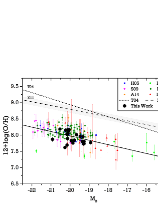
Figure 3: Luminosity-Metallicity Diagram for intermediate star-forming galaxies for objects of this study and comparable samples from the literature. H05 includes 15 luminous star-forming galaxies from DEEP2. K07 includes 7 EELGs, 4 of them are extremely low metallicity galaxies. S09 includes 13 metal-poor galaxies. A14 includes 7 EELGs. L14 includes 16 metal-poor objects. I11 represents a sample of “green peas” with good metallicity determinations. This work presents 22 new metal-poor galaxies. The dashed line represents the luminosity binned LZR by Zahid, Kewley, & Bresolin (2011) (Z11 in the diagram) with a $1-\sigma$ error area. The dotted line on the upper zone of the diagram represents the Tremonti luminosity-metallicity relation for local SDSS galaxies (Tremonti et al. (2004), T04 in the diagram) while the solid line represents the best fit to the combined samples.

We find that our values for luminosities and metallicities are in good agreement with previous determinations, with our error estimates being smaller. Our sample shares the same L-Z locus as the 66 “green peas” from I11, though our galaxies tend to be less luminous and more metal-poor than the “green peas”.

Taken together, all these studies define a locus in the LZR diagram, that is offset from the local LZR of the SDSS sample of Tremonti et al. (2004) towards lower metallicities. These two loci can be represented by linear fits to the data, which are shown in Figure 3; the local fit is represented a dotted line, and the intermediate redshift LZR as a solid line. The linear regressions are:

$$12+\log(O/H) = -0.185(\pm 0.001)M_{B}+5.238(\pm 0.018)$$

$$12+\log(O/H) = -0.135(\pm 0.019)M_{B}+5.272(\pm 0.38)$$

for the local SDSS and intermediate redshift samples respectively.

Both lines have similar slopes, but are offset by a factor of 10 to lower oxygen content for the high luminosity end considered in this work. In principle, this could be due to (i) the different nature of the objects involved, (ii) selection effects regarding both luminosity and chemical abundances, or (iii) a genuine evolutionary effect. However, we should note that the abundances have been derived by two different methods for the local and for the distant samples. The local sample uses empirical calibrations while our work uses direct abundance determinations. The comparison of our $T_{e}$ abundances with those of the intermediate $z$ sample of Zahid, Kewley, & Bresolin (2011), who used empirical calibrations of the oxygen line equivalent widths, is a means of exploring the differences between both methods. Here, it is critical that the parent samples in both works are essentially the same. The luminosity binned LZR, taking the median abundance value as metallicity, by Zahid, Kewley, & Bresolin (2011) is plotted in our Figure 3. It shows that, at the same luminosity, there is an $8-\sigma$ deviation between both abundance distributions. Given the numbers involved in the two samples (about 1700 vs 22), this large deviation implies totally incompatible distributions. This huge discrepancy cannot be solved by taking into account the inherent uncertainties in both methods which amount to 0.2$dex$ at most. This could, in the best scenario, reduce the discrepancy to $4-\sigma$, which is still not plausible.

Our sample also shows similar luminosities, metallicities and optical appearances with the “green peas” population of luminous star forming systems found at lower redshift, although it tends to be fainter and less metal rich than the “green peas”. The full description of the metallicity distribution of star forming systems at intermediate redshift will require the use of IR spectroscopy that allows detecting the [SIII] lines. After carefully considering the systematics of the various metallicity determination methods, we conclude that the metallicity distributions provided by other works like Zahid, Kewley, & Bresolin (2011) and Maier et al. (2014) and the one found in this work are not compatible.

Appendix A DEEP2 Relative flux calibration methods

DEEP2 spectra need to be flux calibrated in order to measure meaningful observational line ratios. Here, we use the results provided by Konidaris (2008) to perform a relative flux calibration of our sample’s spectra. The aim of the relative flux calibration in our paper is to obtain the physical line ratios between oxygen and hydrogen lines by modelling the relative throughput of DEIMOS with wavelength.

Three methods were used to measure relative DEIMOS throughput, which is defined as the number of photons detected at the CCD over the total number of photons that leave the reference object. The basic algorithm to compute the throughput is the same in all the methods and it is the result of dividing a measured stellar spectrum by a standard spectrum associated with it. The three methods used to compute a standard spectrum are: 1) Use a standard-star with well known SED. 2) Use the CFHT photometry to determine the corresponding stellar type in the Gunn-Stryker (G-S) catalog. 3)Use a least-square minimization to determine stellar type in the (G-S) catalog.

After carrying out an analysis of these methods, the throughput can be approximated by a fourth order polynomial:

$y({\lambda})=-77.9026+0.0395916\lambda-7.49911\times 10^{-6}{\lambda}^{-2}$
$+6.29692\times 10^{-10}{\lambda}^{3}-1.97967{\times}10^{-14}{\lambda}^{4}$

where $\lambda$ is wavelength in Å and y($\lambda$) is in units of throughput/Å. The use of the previous calibration yields 10% error in the emission line flux measurements.

References

- Aloisi, Tosi, & Greggio (1999) Aloisi A., Tosi M., Greggio L., 1999, AJ, 118, 302
- Aloisi et al. (2007) Aloisi A., et al., 2007, ApJ, 667, L151
- Amorín et al. (2014) Amorín R., et al., 2014, arXiv, arXiv:1403.3441
- An et al. (2013) An F., Zheng X., Meng Y., Chen Y., Wen Z., Lü G., 2013, SCPMA, 56, 2226
- Asplund et al. (2009) Asplund M., Grevesse N., Sauval A. J., Scott P., 2009, ARA&A, 47, 481
- Bresolin et al. (2005) Bresolin F., Schaerer D., González Delgado R. M., Stasińska G., 2005, A&A, 441, 981
- Campbell (1988) Campbell A., 1988, ApJ, 335, 644
- Cardamone et al. (2009) Cardamone C., et al., 2009, MNRAS, 399, 1191
- Castellanos, Díaz, & Terlevich (2002) Castellanos M., Díaz A. I., Terlevich E., 2002, MNRAS, 329, 315
- Coil et al. (2004) Coil A. L., Newman J. A., Kaiser N., Davis M., Ma C.-P., Kocevski D. D., Koo D. C., 2004, ApJ, 617, 765
- De Robertis, Dufour, & Hunt (1987) De Robertis M. M., Dufour R. J., Hunt R. W., 1987, JRASC, 81, 195
- Diaz (1988) Diaz A. I., 1988, MNRAS, 231, 57
- Díaz et al. (2000) Díaz A. I., Castellanos M., Terlevich E., Luisa García-Vargas M., 2000, MNRAS, 318, 462
- Faber et al. (2003) Faber S. M., et al., 2003, SPIE, 4841, 1657
- French (1980) French H. B., 1980, ApJ, 240, 41
- Hägele et al. (2008) Hägele G. F., Díaz Á. I., Terlevich E., Terlevich R., Pérez-Montero E., Cardaci M. V., 2008, MNRAS, 383, 209
- Hoyos et al. (2005) Hoyos C., Koo D. C., Phillips A. C., Willmer C. N. A., Guhathakurta P., 2005, ApJ, 635, L21
- Hoyos & Díaz (2006) Hoyos C., Díaz A. I., 2006, MNRAS, 365, 454
- Izotov et al. (1994) Izotov, Y. I., Thuan, T. X., & Lipovetsky, V. A. 1994, ApJ, 435, 647
- Izotov, Guseva, & Thuan (2011) Izotov Y. I., Guseva N. G., Thuan T. X., 2011, ApJ, 728, 161
- Kaiser, Squires, & Broadhurst (1995) Kaiser N., Squires G., Broadhurst T., 1995, ApJ, 449, 460
- Kakazu, Cowie, & Hu (2007) Kakazu Y., Cowie L. L., Hu E. M., 2007, ApJ, 668, 853
- Kinkel & Rosa (1994) Kinkel U., Rosa M. R., 1994, A&A, 282, L37
- Kinney et al. (1996) Kinney A. L., Calzetti D., Bohlin R. C., McQuade K., Storchi-Bergmann T., Schmitt H. R., 1996, ApJ, 467, 38
- Konidaris (2008) Konidaris N. P., II, 2008, PhDT, United States - - California: University of California, Santa Cruz; 2008. Publication Number: AAT 3338590. Source: DAI-B 69/12, Jun 2009.
- Lequeux et al. (1979) Lequeux J., Peimbert M., Rayo J. F., Serrano A., Torres-Peimbert S., 1979, A&A, 80, 155
- Ly et al. (2014) Ly C., Malkan M. A., Nagao T., Kashikawa N., Shimasaku K., Hayashi M., 2014, ApJ, 780, 122
- Maier et al. (2014) Maier C., Ziegler B. L., Lilly S. J., Contini T., Pérez-Montero E., Lamareille F., Bolzonella M., Le Floc’h E., 2014, arXiv, arXiv:1410.7389
- Newman et al. (2013) Newman J. A., et al., 2013, ApJS, 208, 5
- Osterbrock & Ferland (2006) Osterbrock, D. E. & Ferland, G. F., 2006, Astrophysics of Gaseous Nebulae and Active Galactic Nuclei Second Edition. University Science Books. ISBN 978-1-891389-34-4.
- Pagel et al. (1992) Pagel B. E. J., Simonson E. A., Terlevich R. J., Edmunds M. G., 1992, MNRAS, 255, 325
- Papaderos et al. (1996) Papaderos P., Loose H.-H., Thuan T. X., Fricke K. J., 1996, A&AS, 120, 207
- Papaderos et al. (2002) Papaderos P., Izotov Y. I., Thuan T. X., Noeske K. G., Fricke K. J., Guseva N. G., Green R. F., 2002, A&A, 393, 461
- Pérez-Montero et al. (2006) Pérez-Montero, E., Díaz, A. I., Vílchez, J. M., & Kehrig, C. 2006, A&A, 449, 193
- Richer & McCall (1995) Richer, M. G., & McCall, M. L. 1995, ApJ, 445, 642
- Searle & Sargent (1972) Searle L., Sargent W. L. W., 1972, ApJ, 173, 25
- Shaw & Dufour (1995) Shaw R. A., Dufour R. J., 1995, PASP, 107, 896
- Salzer, Williams, & Gronwall (2009) Salzer J. J., Williams A. L., Gronwall C., 2009, ApJ, 695, L67
- Stasińska (1990) Stasińska G., 1990, A&AS, 83, 501
- Taylor et al. (1995) Taylor C. L., Brinks E., Grashuis R. M., Skillman E. D., 1995, ApJS, 99, 427
- Tremonti et al. (2004) Tremonti C. A., et al., 2004, ApJ, 613, 898
- Willmer et al. (2006) Willmer C. N. A., et al., 2006, ApJ, 647, 853
- Wirth et al. (2004) Wirth, G. D., et al. 2004, AJ, 127, 3121
- Zahid, Kewley, & Bresolin (2011) Zahid H. J., Kewley L. J., Bresolin F., 2011, ApJ, 730, 137