Spontaneous instabilities and stick-slip motion
in a generalized Hébraud-Lequeux model

Abstract

We revisit the Hébraud-Lequeux (HL) model for the rheology of jammed materials and argue that a possibly important time scale is missing from HL’s initial specification. We show that our generalization of the HL model undergoes interesting oscillating instabilities for a wide range of parameters, which lead to intermittent, stick-slip flows under constant shear rate. The instability we find is akin to the synchronization transition of coupled elements that arises in many different contexts (neurons, fireflies, financial bankruptcies, etc.). We hope that our scenario could shed light on the commonly observed intermittent, serrated flows of glassy materials under shear.

I Introduction

Jammed materials are like Tolstoy’s happy families: they all behave much in the same way. The (non-linear) rheological properties of very different materials such as metallic glasses, foams, dense emulsions or granular packings are remarkably similar. Typically, these materials creep very slowly below a certain yield stress, and exhibit interesting dynamical features such as “avalanches” Baret et al. (2002); Otsuki and Hayakawa (2014) (perhaps similar, at a different scale, to real earthquakes Chen and Bak (1991)) and intermittent, stick-slip like motion, which are still poorly understood – as is the transition from “liquid” flows to “jammed” flows Lerner et al. (2012). At the microscopic scale all of these materials have very different properties and can barely be described by one single model. However on a more coarse grained level, when for example considering rheological or plasticity features, these materials show very similar properties. Such universality has motivated researchers to propose simple phenomenological models to account for them. It is now well accepted that the elementary physical process at play is the yielding of small regions of the material Argon (1979); Princen (1983); Fank and Langer (1998); Langer (2008); Schall and Weitz (2007); Manneville et al. (2004); Amon et al. (2004); Maloney and Lemaire (2006); Tanguy et al. (2006) (the so-called shear transformation zones, STZ), when the local shear stress exceeds some (possibly random) threshold. These STZ are localized but display long-range elastic interactions Picard et al. (2004) that can trigger plastic instabilities. Among the most popular approaches to describe the stochastic collective evolution of these STZ is the Hébraud-Lequeux (HL) model Hébraud and Lequeux (1998), which is a very simple, mean-field description of the elastic interaction between such STZ, in particular how the instability of one of them can trigger the instability of many others (see also Refs. Sollich et al. (1997); Sollich (2006); Jagla et al. (2014); Lieou et al. (2015); Coussot and Overlez (2010) for alternative descriptions and Rodney et al. (2011) for a recent review on this topic). The HL model, in spite of its simplicity, leads to highly non-trivial results, in particular a phase transition between a jammed, arrested phase and a liquid, flowing phase, with a non-linear Herschel-Bulkley law Herschel and Bulkley (1926) for small shear rate in the jammed phase. This model has attracted a renewed interest in the recent years, focusing, inter-alia, on a detailed comparison with the competing Soft-Glassy-Rheology (SGR) models Agoritsas et al. (2015), on avalanche-like dynamics Jagla (2015), and on a generalization of HL that appropriately accounts for the power-law decay of elastic interactions between STZ Lin and Wyart (2015); Lemaitre and Caroli (2007), which deeply modifies the mathematical structure of the exact solution of the model.

In this paper, we revisit the original HL model and argue that some important physical time-scales are missing from its original formulation. Although many of the predictions of HL are unaffected by these modifications, we find that an oscillating instability can appear in some regions of parameter space. We find in particular that the “liquid” phase at zero shear rate is unstable and becomes, close enough the the jammed phase, spontaneously oscillating between a self-sustained liquid and a glass. This instability persists when the shear rate is weak enough, and leads, in physical terms, to an intermittent stick-slip flow (possibly related to so-called serrated flow). Interestingly, oscillatory instabilities also arise in some variants of the SGR models Head, Ajdari and Cates (2001), or within simple phenomenological constitutive equations for shear-thickening materials Aradian and Cates (2006). However, the underlying physical mechanisms leading to instabilities are quite different from the one discussed in the present paper.

The intuition behind our instability in fact comes from a very similar model that we recently studied in the context of economic crisis “waves” and collective bank defaults Gualdi et al. (2015a, b). In all these cases, the common phenomenon is that the instability/default/bankruptcy of a single element can trigger the instabilities of others through interactions. The somewhat surprising feature, however, in that such a coupling can lead to the synchronization of randomly evolving entities, and genuine oscillations – see Strogatz (2003); Gualdi et al. (2015b) and references therein.

The outline of the paper is as follows: we first generalize the HL model such as to describe more accurately what happens when a single entity fails. We then show that the zero shear stationary state computed by HL is linearly unstable to some oscillatory mode in a region of parameters, in particular close to the jamming transition. We then extend our calculation to non-zero shear rates and find the “phase diagram” of the model, in particular we highlight the region where stick-slip motion is expected. We finally conclude and discuss possible extensions of our calculations.

II The model

Let us recall the basic tenets of the HL model Hébraud and Lequeux (1998) and introduce the physical items that we believe are missing from the original framework. Following HL, the material is divided in $N$ regions (or “elements”) labeled by an index $i=1,\cdots,N$, each characterized by a local stress $\sigma_{i}$. The stress $\sigma_{i}$ of each element performs a random walk with:

• a drift $G_{0}\dot{\gamma}$ due to the external shear $\dot{\gamma}$ that loads elastic energy ($G_{0}$ is the elastic shear modulus),

• a time-dependent diffusion $D_{t}$ due to intrinsic noise and elastic interactions between elements.

Whenever $|\sigma_{i}|\geq\sigma_{c}$, the $i$-th element may become unstable, and becomes so at a “plastic” rate $1/\tau_{\rm pl}$. As soon as the element becomes unstable (it is then in a “fluid” state), HL postulates that it re-jams (with $\sigma=0$) immediately in a state of zero stress. We rather assume that it remains in its fluid state during a typical time scale $\tau_{\rm fl}$; in such a state, the element cannot contribute to the shear stress (see also Fig. 1 in Ref. Martens et al. (2012), where $\tau_{\rm fl}$ has been called $\tau_{\rm el}$). With rate $1/\tau_{\rm fl}$, the element re-jams with $\sigma=0$, as in HL. This is a very important ingredient for a correct physical interpretation of the model Martens et al. (2012); Jagla et al. (2014): note that once an element becomes unstable, its dynamics cannot be described by the same drift-diffusion mechanism. On the contrary, when an element becomes unstable, it contributes to the total plastic activity at time $t$, called $\Gamma_{t}$, and increases the diffusion of all other elements identically, in a mean-field way, exactly as in the HL model (see Lin and Wyart (2015) for an improved description). However, we will assume that the plastic activity at time $t$ affects the diffusion coefficient $D_{t}$ with some delay, instead of instantaneously as HL assumed. This reflects, at the mean-field level, the finite propagation speed of information through the sample.

II.1 Mathematical definition of the model

Our modified model can be described by the same Fokker-Planck setting as used by HL Hébraud and Lequeux (1998). The evolution of the (unnormalized) probability $P(\sigma,t)$ to find an element with stress $\sigma$ at time $t$ is given by:

$$\begin{split}\dot{P}(\sigma,t)&=D_{t}P^{\prime\prime}(\sigma,t)-G_{0}\dot{\gamma}P^{\prime}(\sigma,t)\\ &+J_{t}\delta(\sigma)-\frac{1}{\tau_{\rm pl}}P(\sigma,t)H(|\sigma|-\sigma_{c})\ ,\end{split}$$ (1)

where $H(x)$ is the Heaviside step function, and with:

$$\begin{split}J_{t}&=\frac{1}{\tau_{\rm fl}}(1-\phi_{t})\ ,\\ \phi_{t}&=\int_{-\infty}^{\infty}d\sigma\,P(\sigma,t)\ ,\\ \Gamma_{t}&=\frac{1}{\tau_{\rm pl}}\int_{|\sigma|\geq\sigma_{c}}d\sigma\,|\sigma|P(\sigma,t)\ ,\\ D_{t}&=D_{\rm int}+\alpha\omega\int_{-\infty}^{t}ds\,\,e^{-\omega(t-s)}\Gamma_{s}\ .\end{split}$$ (2)

Here, $\phi_{t}$ is the fraction of jammed elements that contribute to the elastic stress and $J_{t}$ is the flux of elements that re-jam between $t$ and $t+{\rm d}t$, initially at zero stress. One can assume for simplicity that the fraction of fluidized elements, $(1-\phi_{t})$, contributes a viscous stress proportional to $\dot{\gamma}$. Hence, the total stress is

$$\Sigma_{t}=\int_{-\infty}^{\infty}d\sigma\,\sigma\,P(\sigma,t)+(1-\phi_{t})\eta\dot{\gamma}\ ,$$ (3)

where $\eta$ is the microscopic viscosity of the fluid elements. Note that $\phi_{t}$ satisfies the equation:

$$\dot{\phi}_{t}=\frac{1}{\tau_{\rm fl}}(1-\phi_{t})-\frac{1}{\tau_{\rm pl}}\int_{|\sigma|\geq\sigma_{c}}d\sigma P(\sigma,t)\ .$$ (4)

The equation for $D_{t}$ means that yielding events, when they happen, impose an extra random stress onto other elements but with some time lag that we model as an exponential kernel, with a coupling constant $\alpha$. $D_{\rm int}$ is an intrinsic noise term (for example temperature) that we will choose to be very small in the following. Furthermore we choose $G_{0}=1$ without loss of generality. The control parameters for this model are $\sigma_{c},\dot{\gamma},\tau_{\rm fl},\tau_{\rm pl},D_{\rm int},\alpha,\omega$. Because one can fix arbitrarily the units of $\sigma$ and of $t$, there are in fact four plus one independent adimensional control parameters: for example $\widehat{\gamma}:=\dot{\gamma}\tau_{\rm fl}/\sigma_{c}$, $\alpha$, $\tau_{\rm pl}/\tau_{\rm fl}$, $\widehat{\omega}:=\omega\tau_{\rm fl}$, and finally $\text{Pe}:=\dot{\gamma}\sigma_{c}/D_{\rm int}\rightarrow\infty$ throughout this paper.

II.2 Connection with the Hébraud-Lequeux model

The standard HL model is recovered if we set $D_{\rm int}=0$, $\tau_{\rm fl}=0$ and $\omega=\infty$, i.e: no intrinsic noise, fluid regions re-jam instantaneously, and yielding elements affect the stress of other regions instantaneously as well. In the HL limit $\tau_{\rm fl}=0$, we therefore have $\dot{\phi}_{t}=0$ and $\phi_{t}\equiv 1$, and from Eq. (4) we have $J_{t}=\frac{1}{\tau_{\rm pl}}\int_{|\sigma|\geq\sigma_{c}}d\sigma P(\sigma,t)$. For $D_{\rm int}=0$ and $\omega\rightarrow\infty$, we indeed recover HL’s prescription $D_{t}=\alpha\Gamma_{t}$. Summarizing, we obtain Eq. (1) with

$$\begin{split}J_{t}&=\frac{1}{\tau_{\rm pl}}\int_{|\sigma|\geq\sigma_{c}}d\sigma P(\sigma,t)\ ,\\ D_{t}&=\alpha\Gamma_{t}=\frac{\alpha}{\tau_{\rm pl}}\int_{|\sigma|\geq\sigma_{c}}d\sigma|\sigma|P(\sigma,t)\ .\end{split}$$ (5)

This coincides with the HL model, with the only difference that $\Gamma_{t}$ is defined without the $|\sigma|$. Although this does not make any important difference in the properties of the model, in particular the instability described below, we argue that our definition has a more precise physical interpretation, since the plastic activity should be the average of $|\sigma|$. In conclusion, the presence of the additional time scales $\tau_{\rm fl}$ and $1/\omega$ is the main difference between our model and HL, and we will see that they play a crucial role in the physics of the model.

II.3 The limit $\tau_{\rm pl}\rightarrow 0$

For the ease of analytical calculations, we will set in the following $\tau_{\rm pl}=0$, which means that an element becomes unstable immediately when $|\sigma|>\sigma_{c}$, while keeping a finite fluid lifetime $\tau_{\rm fl}$. The HL model corresponds to the opposite limit $\tau_{\rm pl}/\tau_{\rm fl}\rightarrow\infty$, but it is reasonable to expect that in many applications the ratio $\tau_{\rm pl}/\tau_{\rm fl}$ can take very different values, from quite small to quite large. In this paper we examine analytically the limit $\tau_{\rm pl}/\tau_{\rm fl}\ll 1$, and numerically the regime where $\tau_{\rm pl}/\tau_{\rm fl}\sim 1$. For small $\tau_{\rm pl}/\tau_{\rm fl}$ we find an oscillating instability, which disappears when $\tau_{\rm pl}/\tau_{\rm fl}$ exceeds a (parameter dependent) threshold value, simply because the synchronisation effect reported below cannot set in. So strictly speaking, the instability reported here is absent in the original HL setting.

When $\tau_{\rm pl}=0$, Eq. (1) is simply complemented by an absorbing boundary condition at $|\sigma|=\sigma_{c}$, implying $P(|\sigma|=\sigma_{c})=0$. Furthermore, the plastic activity is given by the number of regions that become unstable per unit time, hence in Eq. (2) $\Gamma_{t}$ is given by the outgoing flux at $\pm\sigma_{c}$, i.e.:

$$\Gamma_{t}=\sigma_{c}D_{t}[P^{\prime}(-\sigma_{c},t)-P^{\prime}(\sigma_{c},t)]\ .$$ (6)

Note that in this limit the difference in our definition of $\Gamma_{t}$ with respect to HL becomes irrelevant, because $|\sigma|=\sigma_{c}$ is the only contribution to $\Gamma_{t}$. For simplicity, we also set $\sigma_{c}=1$ in the following.

III Vanishing shear rate

We will consider first the situation with no external shear, i.e. $\dot{\gamma}=0$. It turns out that the interesting limit corresponds to the case when the intrinsic activity tends to zero, i.e. $D_{\rm int}\rightarrow 0$, as in the HL model. The only two adimensional control parameters left are thus $\alpha$ and $\widehat{\omega}:=\omega\tau_{\rm fl}$.

Note that, as we will show in the following (Sect. IV.1), for $\alpha<1/2$ and $D_{\rm int}=0$ there is a history-dependent jammed phase in which the material can self-sustain, in the $\dot{\gamma}=0$ limit, any finite stress within the interval $[-\sigma_{c},+\sigma_{c}]$. In this case, setting directly $\dot{\gamma}=0$ as we do below corresponds to a particular choice of history such that stationary stress distribution is symmetric and the average stress is zero. The main point of this section is to illustrate our calculation in the simplest possible case.

III.1 The stationary solution: a jamming transition

We thus look for a stationary solution of Eq. (1) with $P(\sigma,t)=P_{0}(\sigma)$, $J_{t}=J_{0}$, etc., which in this case is particularly simple and reads:

$$P_{0}(\sigma>0)=A(1-\sigma)\ ,\qquad P_{0}(-\sigma)=P_{0}(\sigma)\ ,$$ (7)

with the discontinuity of the slope at the origin related to $J_{0}$ by Eq. (1) as $2D_{0}A=J_{0}$. The fraction of active elements $\phi_{0}=\int_{-1}^{1}d\sigma P_{0}(\sigma)$ is simply given by $A$, so that from Eq. (2)

$$J_{0}=\frac{1}{\tau_{\rm fl}}(1-A)\hskip 10.0pt\longrightarrow\hskip 10.0ptA=\frac{1}{2D_{0}\tau_{\rm fl}+1}\ .$$ (8)

Eq. (6) gives $\Gamma_{0}=2AD_{0}$ and from Eq. (1) we get $D_{0}=D_{\rm int}+\alpha\Gamma_{0}=D_{\rm int}+2\alpha AD_{0}$. We thus obtain a self-consistent equation for the stationary value of the diffusion coefficient

$$2D_{0}^{2}\tau_{\rm fl}-2D_{0}(\delta\alpha+D_{\rm int}\tau_{\rm fl})-D_{\rm int}=0\ ,$$ (9)

where $\delta\alpha=\alpha-1/2$. This second degree equation has two possible solutions that read, in the limit $D_{\rm int}\rightarrow 0$:

$$D_{0}^{-}=-\frac{D_{\rm int}}{2\delta\alpha}\ ;\qquad D_{0}^{+}=\frac{2\delta\alpha}{2\tau_{\rm fl}}+\frac{\alpha D_{\rm int}\tau_{\rm fl}}{4\delta\alpha}\ ,$$ (10)

where clearly the first solution holds for $\alpha<1/2$ and the second holds for $\alpha>1/2$. When $D_{\rm int}\rightarrow 0$ there is, as first noted by HL, a transition between a fluid phase $\alpha>1/2$ where activity is self sustained $D_{0}^{+}>0$, and a jammed phase $\alpha<1/2$ where activity is absent, $D_{0}^{-}=0$, see Fig. 1 and Ref. Agoritsas et al. (2015). In the jammed phase, one has $A=1$ and in the liquid phase, $A=1/(2\alpha)$, to leading order in $D_{\rm int}$.

III.2 Linear stability analysis

Following Gualdi et al. (2015b), we are interested in studying the stability of the stationary solution with respect to a linear perturbation. We thus write $P(\sigma,t)=P_{0}(\sigma)+\varepsilon P_{1}(\sigma,t)$, $D_{t}=D_{0}+\varepsilon D_{1}(t)$, $\phi_{t}=\phi_{0}+\varepsilon\phi_{1}(t)$. Linearizing Eq. (1) we get

$$\dot{P}_{1}(\sigma,t)=D_{0}P_{1}^{\prime\prime}(\sigma,t)+D_{1}(t)P_{0}^{\prime\prime}(\sigma)-\frac{1}{\tau_{\rm fl}}\phi_{1}(t)\delta(\sigma)\ ,$$ (11)

with the boundary conditions $P_{1}(\sigma=\pm 1,t)=0$. Therefore,

$$\begin{split}P_{1}(\sigma,t)&=\int_{0}^{\infty}d\tau\int_{-1}^{1}d\bar{\sigma}\,G(\sigma,t|\bar{\sigma},t-\tau)\\ &\times\left[D_{1}(t-\tau)P_{0}^{\prime\prime}(\bar{\sigma})-\frac{1}{\tau_{\rm fl}}\phi_{1}(t-\tau)\delta(\bar{\sigma})\right]\ .\end{split}$$ (12)

where $P_{0}^{\prime\prime}(\sigma)=-2A\delta(\sigma)$, and $G$ is the random walk propagator in the interval $[-1,+1]$.

Combining Eqs. (2) and (6), setting $D_{\rm int}=0$ in the linear regime we obtain an equation for the diffusion constant $D_{1}(t)$:

$$\begin{split}D_{1}(t)&=\alpha\omega\int_{-\infty}^{t}dsD_{0}\left[P_{1}^{\prime}(-1,s)-P_{1}^{\prime}(1,s)\right]e^{-\omega(t-s)}\\ &+2A\alpha\omega\int_{-\infty}^{t}dsD_{1}(s)e^{-\omega(t-s)}\ .\end{split}$$ (13)

Exponentials of time, with $D_{1}(t)={\cal D}e^{\lambda t}$, $\phi_{1}(t)=\Phi e^{\lambda t}$, $P_{1}^{\prime}(-1,t)=-P_{1}^{\prime}(1,t)=\Pi e^{\lambda t}$, are consistent solutions of the linearized equations. We find from Eq. (13):

$${\cal D}=\frac{2\alpha\omega D_{0}}{\omega(1-2\alpha A)+\lambda}\Pi\ .$$ (14)

In order to compute $P_{1}(\sigma,t)$ simply, one can notice that $H_{\bar{\sigma}}(\sigma,\lambda)=\int_{0}^{\infty}d\tau e^{-\lambda\tau}G(\sigma,\tau|\bar{\sigma},0)$ obeys the following partial differential equation:

$$D_{0}H_{\bar{\sigma}}^{\prime\prime}(\sigma,\lambda)-\lambda H_{\bar{\sigma}}(\sigma,\lambda)=-\delta(\sigma-{\bar{\sigma}})\ ,$$ (15)

with boundary condition $H_{\bar{\sigma}}(\sigma=\pm 1,\lambda)=0$. Specializing to ${\bar{\sigma}}=0$, one finds:

$$\begin{split}&H(\sigma>0,\lambda)=\widehat{A}\left[e^{-\kappa\sigma}-e^{-2\kappa}e^{\kappa\sigma}\right]\ ,\\ &H(-\sigma,\lambda)=H(\sigma,\lambda)\end{split}$$ (16)

with $\kappa^{2}=\lambda/D_{0}$. The discontinuity of the first derivative at the origin gives:

$$2D_{0}\widehat{A}=\frac{1}{\kappa(1+e^{-2\kappa})}\ ,$$ (17)

so finally $H^{\prime}(-1,\lambda)=-H^{\prime}(1,\lambda)=1/(2D_{0}\cosh\kappa)$. Plugging this in the general expression for $P_{1}(\sigma,t)$ in Eq. (12), taking the derivative with respect to $\sigma$ and setting $\sigma=-1$ finally leads to:

$$\Pi=-\frac{1}{2D_{0}\cosh\kappa}\left[2A{\cal D}+\frac{1}{\tau_{\rm fl}}\Phi\right].$$ (18)

Finally, integrating Eq. (11) over $\sigma$ leads to:

$$\lambda\Phi=-\frac{1}{\tau_{\rm fl}}\Phi-2D_{0}\Pi-2{\cal D}A\ .$$ (19)

In the liquid phase ($D_{0}>0$ and $A=1/(2\alpha)$) the solvability condition of the system of Eqs. (14), (18), (19) relating ${\cal D},\Pi$ and $\Phi$ finally reads, in terms of $\widehat{\lambda}=\lambda\tau_{\rm fl}$ and $\widehat{\omega}=\omega\tau_{\rm fl}$:

$$1+\widehat{\lambda}=\frac{\widehat{\omega}+\widehat{\lambda}}{\widehat{\omega}+\widehat{\lambda}\cosh\sqrt{\frac{\widehat{\lambda}}{\delta\alpha}}}\ ,$$ (20)

or equivalently (for $\widehat{\lambda}\neq 0$)

$$\widehat{\omega}=1-(1+\widehat{\lambda})\cosh\sqrt{\frac{\widehat{\lambda}}{\delta\alpha}}\ .$$ (21)

If all the solutions of Eq. (21) have a negative real part, the stationary solution is stable, while it is unstable otherwise. This condition defines the transition point $\alpha_{\rm c}(\widehat{\omega})$. Note that for $\alpha\rightarrow\infty$ we obtain from Eq. (21) that $\widehat{\lambda}=-\widehat{\omega}$ and therefore the stationary state is stable.

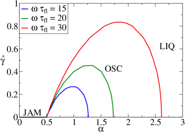
Figure 1: Top: Phase diagram of the model in the $(\alpha,\widehat{\gamma})$ plane (recall that $\widehat{\gamma}=\dot{\gamma}\tau_{\rm fl}$) obtained from the solutions of Eq. (44) with $D_{i}\rightarrow 0$ and different values of $\widehat{\omega}=\omega\tau_{\rm fl}$. In the liquid (LIQ) phase, the system is stationary, and the flow curve is basically Newtonian in the whole range of $\widehat{\gamma}$. In the jammed (JAM) phase, the system has a finite yield stress for $\widehat{\gamma}\rightarrow 0$. Finally, in the oscillating (OSC) phase, the stress is an oscillating function of time. Bottom: Flow curves displaying the average stress versus strain for $\widehat{\omega}=20$, $D_{\rm int}=0.005$, and three different values of $\alpha$ corresponding to the jammed, oscillating, and liquid phases. Points correspond to numerical results while lines correspond to analytical results for the stationary state. For $\alpha=2.5$ the system is liquid and the flow curve is Newtonian in all the regimes of $\widehat{\gamma}$. For $\alpha=0.25$ the system is jammed for $\widehat{\gamma}\rightarrow 0$ and the stress tends to a finite value (dotted line), but in the simulation due to finite $D_{\rm int}$ we also see a Newtonian regime at small $\widehat{\gamma}$ (points and dashed line). For $\alpha=1.25$ the system is oscillating for small $\widehat{\gamma}$: in this case we report the minimum, average and maximum value of the stress (see Fig. 2 for an example).

III.3 Large $\omega$ analysis

Eq. (21) can be analyzed in the limit of large $\omega$ (that corresponds to the HL case where stress propagation is instantaneous throughout the sample), assuming that $\alpha_{\rm c}(\widehat{\omega})$ and $\widehat{\lambda}$ are also large (we will see that they are proportional to $\widehat{\omega}$). We obtain

$$\widehat{\omega}=-\widehat{\lambda}\cosh\sqrt{\frac{\widehat{\lambda}}{\alpha}}\ .$$ (22)

Let us assume that at the transition there is a single unstable mode whose real part crosses zero continuously. Thus $\widehat{\lambda}=i\lambda_{\rm I}$ is pure imaginary at $\alpha_{\rm c}$. In this case, for the r.h.s. of Eq. (22) to be real we need $\cos\sqrt{\lambda_{\rm I}/(2\alpha)}=0$ which implies $\lambda_{\rm I}=\alpha\pi^{2}(1+2n)^{2}/2$ with $n\in\hbox{\msytw Z}$. Then we get

$$\frac{\widehat{\omega}}{\alpha}=(-1)^{n}\frac{\pi^{2}}{2}(1+2n)^{2}\sinh\left(\frac{\pi}{2}(1+2n)\right)\ .$$ (23)

Because the system is stable at $\alpha\rightarrow\infty$, the stability boundary corresponds to the largest value of $\alpha$ for which a mode is unstable, and thus to the smallest value of the r.h.s. of Eq. (23), which is assumed for $n=0$ and gives

$$\frac{\alpha_{\rm c}(\widehat{\omega})}{\widehat{\omega}}=\frac{2}{\pi^{2}\sinh\left(\frac{\pi}{2}\right)}=0.088055\ldots\ ,$$ (24)

in excellent agreement with the numerical results of Fig. 1 when $\widehat{\omega}$ is large enough (for example, $\widehat{\omega}=30$ should correspond to $\alpha_{\rm c}\approx 2.64$).

III.4 Summary

Let us summarize the content of this section. We discussed the case of vanishing shear rate, $\dot{\gamma}=0$, and intrinsic activity, $D_{\rm int}\rightarrow 0$, assuming $\tau_{\rm pl}\ll\tau_{\rm fl}$. The control parameters are $\alpha$ and $\widehat{\omega}=\omega\tau_{\rm fl}$. We found that:

• For $\alpha<1/2$, the system is jammed: no motion occurs as $D_{t}\equiv 0$.

• For $\alpha>\alpha_{\rm c}(\widehat{\omega})\approx\widehat{\omega}\times 0.088055\ldots$, there is a stationary “liquid” phase with self-sustained activity, $D_{t}\equiv D_{0}>0$.

• For $1/2<\alpha<\alpha_{\rm c}(\widehat{\omega})$ the liquid phase is in fact unstable; in this case, as shown in Fig. 2, the system undergoes spontaneous oscillations between periods where the number of fluid elements is large and periods where it is small. When an external shear is applied, this state will correspond to intermittent, stick-slip motion.

Let us emphasize that the liquid phase of the model is unphysical in the strict limit $D_{\rm int}=0$ and $\dot{\gamma}=0$, because no motion is possible in this case. However, one can think that $D_{\rm int}$ is very small but finite, modeling some external noise (e.g. a small temperature), or that $\dot{\gamma}\rightarrow 0^{+}$. As we discuss next, the more interesting case $\dot{\gamma}>0$ is indeed perfectly regular in the limit where $\dot{\gamma}\rightarrow 0$.

IV Non-zero shear rate

We now generalize the calculation to a non-zero external shear, $\dot{\gamma}\neq 0$, still in the limit $D_{\rm int}\rightarrow 0$. In addition to $\alpha$ and $\widehat{\omega}=\omega\tau_{\rm fl}$, there is now a third control parameter $\widehat{\gamma}=\dot{\gamma}\tau_{\rm fl}$. We also define $\zeta=\dot{\gamma}\sigma_{c}/D_{0}$, which is an adimensional “renormalized Péclet number” quantifying the importance of drift with respect to the steady-state diffusion constant in Eq. (1). Remember however that we set $\sigma_{c}=1$ henceforth.

IV.1 The stationary case

The stationary solution now reads:

$$\begin{split}P_{0}(\sigma>0)&=A(1-e^{-\zeta(1-\sigma)})\ ,\\ P_{0}(\sigma<0)&=-Ae^{-\zeta}(1-e^{\zeta(1+\sigma)})\ .\end{split}$$ (25)

Integrating Eq. (1) one can relate the discontinuity of the slope at the origin to $J_{0}$ as $A=\frac{J_{0}}{\dot{\gamma}}\frac{1}{1+e^{-\zeta}}$. Moreover, the fraction of active elements is $\phi_{0}=A(1-e^{-\zeta})$, and $J_{0}=(1-\phi_{0})/\tau_{\rm fl}$. We thus have three equations for $J_{0}$, $\phi_{0}$ and $A$ and the solution is

$$J_{0}=\frac{\dot{\gamma}}{\dot{\gamma}\tau_{\rm fl}+\tanh(\zeta/2)}\ ,$$ (26)

from which we obtain $\phi_{0}$ and $A$ thus completing the calculation of $P_{0}(\sigma)$.

From $P_{0}(\sigma)$ we obtain the self-consistent equation obeyed by $D_{0}=\dot{\gamma}/\zeta$. Combining Eqs. (2) and (6), we have $D_{0}=D_{\rm int}+\alpha\Gamma_{0}=D_{\rm int}+\alpha D_{0}[P_{0}^{\prime}(-1)-P_{0}^{\prime}(1)]$. For $D_{\rm int}\rightarrow 0$ we obtain:

$$\frac{D_{0}}{\dot{\gamma}}=\frac{1}{\zeta}=\frac{\alpha}{\widehat{\gamma}+\tanh(\zeta/2)}\ ,$$ (27)

which is more conveniently written as

$$\widehat{\gamma}+\tanh(\zeta/2)=\alpha\zeta\ .$$ (28)

One is now always in a “liquid” phase with a finite diffusion constant $D_{0}>0$, induced by the shear rate.

We can also compute the average stress. We obtain from Eq. (3)

$$\Sigma_{0}=\frac{\zeta-2+(\zeta+2)e^{-\zeta}}{2\alpha\zeta^{2}(1+e^{-\zeta})}+\widehat{\eta}\frac{\widehat{\gamma}^{2}}{\alpha\zeta}\ ,$$ (29)

where $\widehat{\eta}=\eta/\tau_{\rm fl}$. Note that for large $\widehat{\gamma}$, Eq. (28) gives $\zeta\sim\widehat{\gamma}/\alpha$ and thus $\Sigma_{0}\sim\widehat{\eta}\,\widehat{\gamma}$ is always Newtonian, begin dominated by the fluidized elements. A plot of $\Sigma_{0}$ versus $\widehat{\gamma}$ for several values of $\alpha$ is reported in Fig. 1.

Note that the behavior at small $\dot{\gamma}$ is very different when $\alpha>1/2$ or when $\alpha<1/2$. In the limit $\widehat{\gamma}\rightarrow 0$:

• For $\alpha>1/2$, it is easy to see graphically that Eq. (28) has a unique solution for $\zeta$ for all $\widehat{\gamma}$, and that $\zeta\sim\widehat{\gamma}/\delta\alpha\rightarrow 0$. Hence, Eq. (25) reduces to Eq. (7). Furthermore,

  $$D_{0}=\widehat{\gamma}/(\zeta\tau_{\rm fl})\rightarrow\delta\alpha/\tau_{\rm fl}=D_{0}^{+}$$ (30)

  as in Eq. (10), while the stress

  $$\Sigma_{0}\sim\frac{\widehat{\gamma}}{\alpha}\left(\frac{1}{24\delta\alpha}+\widehat{\eta}\delta\alpha\right)$$ (31)

  is Newtonian, but with a very different prefactor from the large $\widehat{\gamma}$ regime.

• For $\alpha\leq 1/2$, one finds instead that Eq. (28) has multiple solutions when $\widehat{\gamma}$ is small enough. Yet at large $\widehat{\gamma}$ the solution is unique and reducing $\widehat{\gamma}$ gradually one sees that $\forall\widehat{\gamma}>0$ the largest solution for $\zeta$ has to be chosen. This solution for $\zeta$ remains finite for $\dot{\gamma}\rightarrow 0$. Consequently, Eq. (25) does not reduce to Eq. (7), which shows that for $\alpha\leq 1/2$ one cannot set $\dot{\gamma}=0$ directly because the limit is singular. Setting directly $\dot{\gamma}=0$ as in Sec. III corresponds to choosing a particular solution, corresponding to $\Sigma_{0}=0$, which is therefore not the physically natural solution, obtained by preparing the system under shear and reducing progressively $\dot{\gamma}$ to zero. In the latter case, $D_{0}\propto\widehat{\gamma}$ and $\Sigma_{0}$ remains finite when $\dot{\gamma}\rightarrow 0$: the system is jammed, has no plastic activity and can sustain a finite stress even for $\dot{\gamma}=0$.

Note that $\zeta\rightarrow 0$ for $\alpha\rightarrow 1/2^{-}$. Thus $D_{0}=D_{0}^{+}+O(\dot{\gamma}^{2})$ for $\alpha>1/2$ – see also Agoritsas et al. (2015).

IV.2 Linear stability analysis

We linearize once again Eq. (1) with $P(\sigma,t)=P_{0}(\sigma)+\varepsilon P_{1}(\sigma,t)$, $D_{t}=D_{0}+\varepsilon D_{1}(t)$, $\phi_{t}=\phi_{0}+\varepsilon\phi_{1}(t)$. The linearized equation reads:

$$\begin{split}\dot{P}_{1}(\sigma,t)&=D_{0}P_{1}^{\prime\prime}(\sigma,t)-\dot{\gamma}P_{1}^{\prime}(\sigma,t)\\ &+D_{1}(t)P_{0}^{\prime\prime}(\sigma)-\frac{1}{\tau_{\rm fl}}\phi_{1}(t)\delta(\sigma)\ ,\end{split}$$ (32)

with the boundary conditions $P_{1}(\sigma=\pm 1,t)=0$. Therefore

$$\begin{split}P_{1}(\sigma,t)&=\int_{0}^{\infty}d\tau\int_{-1}^{1}d\bar{\sigma}\,G_{\dot{\gamma}}(\sigma,t|\bar{\sigma},t-\tau)\\ &\times\left[D_{1}(t-\tau)P_{0}^{\prime\prime}(\bar{\sigma})-\frac{1}{\tau_{\rm fl}}\phi_{1}(t-\tau)\delta(\bar{\sigma})\right]\ ,\end{split}$$ (33)

where $G_{\dot{\gamma}}$ is the biased random walk propagator in the interval $[-1,+1]$. The diffusion constant $D_{1}(t)$ satisfies:

$$\begin{split}D_{1}(t)&=\alpha\omega\int_{-\infty}^{t}dsD_{0}\left[P_{1}^{\prime}(-1,s)-P_{1}^{\prime}(1,s)\right]e^{-\omega(t-s)}\\ &+\frac{J_{0}}{D_{0}}\alpha\omega\int_{-\infty}^{t}dsD_{1}(s)e^{-\omega(t-s)}\ .\end{split}$$ (34)

Assuming exponential (in time) solutions with $D_{1}(t)={\cal D}e^{\lambda t}$, $\phi_{1}(t)=\Phi e^{\lambda t}$, $P_{1}^{\prime}(\pm 1,t)=\mp\Pi_{\pm}e^{\lambda t}$, we find from Eq. (34):

$${\cal D}=\frac{\alpha\omega D_{0}}{\omega(1-\alpha J_{0}/D_{0})+\lambda}(\Pi_{+}+\Pi_{-})\ .$$ (35)

Integrating Eq. (32) over $\alpha$ and using $P_{1}(\sigma=\pm 1,t)=0$ leads to:

$$\lambda\Phi=-\frac{1}{\tau_{\rm fl}}\Phi-D_{0}(\Pi_{+}+\Pi_{-})-{\cal D}\frac{J_{0}}{D_{0}}\ .$$ (36)

In order to compute $P_{1}(\sigma,t)$ simply, one can notice that $H_{\bar{\sigma}}(\sigma,\lambda;\dot{\gamma})=\int_{0}^{\infty}d\tau e^{-\lambda\tau}G_{\dot{\gamma}}(\sigma,\tau|\bar{\sigma},0)$ obeys the following equation:

$$D_{0}H_{\bar{\sigma}}^{\prime\prime}(\sigma,\lambda;\dot{\gamma})-\dot{\gamma}H_{\bar{\sigma}}^{\prime}(\sigma,\lambda;\dot{\gamma})-\lambda H_{\bar{\sigma}}(\sigma,\lambda;\dot{\gamma})=-\delta(\sigma-\bar{\sigma})\ ,$$

with boundary condition $H_{\bar{\sigma}}(\sigma=\pm 1,\lambda;\dot{\gamma})=0$. We will denote $\kappa_{\pm}$ the two real roots of the equation:

$$D_{0}\kappa^{2}-\dot{\gamma}\kappa-\lambda=0\ ,$$ (37)

and $\Delta=\kappa_{+}-\kappa_{-}$. The solution then reads, respectively for $\sigma>\bar{\sigma}$ and $\sigma<\bar{\sigma}$:

$$H_{\bar{\sigma}}(\sigma,\lambda;\dot{\gamma})=A_{\pm}({\bar{\sigma}})e^{\kappa_{+}\sigma}+B_{\pm}({\bar{\sigma}})e^{\kappa_{-}\sigma}\ ,$$ (38)

with the following equations coming from boundary conditions:

$$\begin{split}&A_{\pm}e^{\pm\kappa_{+}}=-B_{\pm}e^{\pm\kappa_{-}}\Rightarrow B_{\pm}=-A_{\pm}e^{\pm\Delta}\ ,\\ &(A_{+}-A_{-})e^{\kappa_{+}{\bar{\sigma}}}+(B_{+}-B_{-})e^{\kappa_{-}{\bar{\sigma}}}=0\ ,\\ &\kappa_{+}(A_{+}-A_{-})e^{\kappa_{+}{\bar{\sigma}}}+\kappa_{-}(B_{+}-B_{-})e^{\kappa_{-}{\bar{\sigma}}}=-\frac{1}{D_{0}}\ .\end{split}$$ (39)

Solving for $A_{\pm}$ yields:

$$A_{\pm}({\bar{\sigma}})=\frac{e^{\mp\Delta-\kappa_{+}{\bar{\sigma}}}-e^{-\kappa_{-}{\bar{\sigma}}}}{2D_{0}\Delta\sinh\Delta}.$$ (40)

The relevant quantities here are $H_{\bar{\sigma}}^{\prime}(\sigma=\pm 1,\lambda;\dot{\gamma})$, which are expressed as:

$$\begin{split}H_{\bar{\sigma}}^{\prime}(\sigma=\pm 1,\lambda;\dot{\gamma})&=\kappa_{+}A_{\pm}({\bar{\sigma}})e^{\pm\kappa_{+}}+\kappa_{-}B_{\pm}({\bar{\sigma}})e^{\pm\kappa_{-}}\\ &=A_{\pm}({\bar{\sigma}})\Delta e^{\pm\kappa_{+}}\ .\end{split}$$

Using

$$\begin{split}&D_{0}P_{0}^{\prime\prime}(\sigma)=\dot{\gamma}P_{0}^{\prime}(\sigma)-J_{0}\delta(\sigma)\ ,\\ &P_{0}^{\prime}(\sigma>0)=-A\zeta e^{-\zeta(1-\sigma)},\qquad P_{0}^{\prime}(\sigma<0)=A\zeta e^{\zeta\sigma}\ ,\end{split}$$

in Eq. (33), one finds two contributions. The one coming from $\delta(\bar{\sigma})$ reads:

$$\Pi_{\pm}^{\delta}=\pm\left(\frac{J_{0}{\cal D}}{D_{0}}+\frac{1}{\tau_{\rm fl}}\Phi\right)\frac{e^{\pm\kappa_{-}}-e^{\pm\kappa_{+}}}{2D_{0}\sinh\Delta}\ ,$$ (41)

while the continuous part gives:

$$\Pi_{\pm}^{c}=\mp\frac{\dot{\gamma}{\cal D}}{D_{0}}\Delta e^{\pm\kappa_{+}}\int_{-1}^{+1}{\rm d}{\bar{\sigma}}P_{0}^{\prime}({\bar{\sigma}})A_{\pm}({\bar{\sigma}})\ .$$ (42)

From these we deduce:

$$\begin{split}\Pi_{+}^{\delta}+\Pi_{-}^{\delta}&=\left(\frac{J_{0}{\cal D}}{D_{0}}+\frac{1}{\tau_{\rm fl}}\Phi\right)\frac{\sinh\kappa_{-}-\sinh\kappa_{+}}{D_{0}\sinh\Delta}\ ,\\ \Pi_{+}^{c}+\Pi_{-}^{c}&=-\frac{J_{0}{\cal D}\zeta}{D_{0}^{2}\kappa_{+}\kappa_{-}}\frac{(e^{-\kappa_{+}}-1)(e^{-\kappa_{-}}-1)}{e^{-\zeta}+1}\times\\ &\times\frac{\kappa_{+}\sinh\kappa_{-}-\kappa_{-}\sinh\kappa_{+}}{\sinh\Delta}\ .\end{split}$$ (43)

We now have all the elements to obtain the solvability condition of the three equations (35), (36), and (43), relating ${\cal D},(\Pi_{+}+\Pi_{-})$ and $\Phi$, in terms of $\widehat{\lambda}=\lambda\tau_{\rm fl}$, $\widehat{\omega}=\omega\tau_{\rm fl}$ and $\widehat{\gamma}=\dot{\gamma}\tau_{\rm fl}$. We obtain the condition

$$\begin{split}&\frac{\widehat{\lambda}}{\widehat{\omega}}\left(1-\frac{\widehat{\omega}-1}{\widehat{\lambda}+1}\right)=\frac{-\zeta}{e^{-\zeta}+1}\frac{(e^{-\kappa_{-}}-1)(e^{-\kappa_{+}}-1)}{\kappa_{+}\kappa_{-}}\times\\ &\times\frac{\kappa_{+}\sinh{\kappa_{-}}-\kappa_{-}\sinh{\kappa_{+}}}{\sinh{(\kappa_{-})}-\sinh{(\kappa_{+})}}\ .\end{split}$$ (44)

The location of the oscillatory instability in the $(\alpha,\widehat{\gamma})$ plane, as predicted by the above equation, forms a kind of “bubble” region as shown in Fig.  1. We see that for all $\alpha\in[1/2,\alpha_{c}]$ where the zero-shear state is unstable, there exists a critical shear-stress $\dot{\gamma}_{c}$ beyond which the flow is stabilized and becomes laminar. Conversely, coming from high shear, there is a shear-stress $\dot{\gamma}_{c}$ below which the flow becomes intermittent, or stick-slip. This stick-slip phenomenon only exists if the elastic coupling between elements is neither too large, nor too small.

V Numerical results

The linear stability analysis derived in the previous sections is in very good agreement with numerical simulations of the model with a discrete number of elements. In order to obtain numerical results we take a set of $N$ elements characterized by continuous stress variables $\{\sigma_{i}(t)\}_{i=1\cdots N}$ and boolean variables $\{y_{i}(t)\}_{i=1\cdots N}$ (indicating if the element is jammed or is fluidized). At the beginning of each time step the $\sigma_{i}$ of jammed elements are first independently updated by generating Gaussian distributed increments with mean $-\dot{\gamma}\mathrm{d}t$ and round mean square $\sqrt{2\mathrm{d}tD_{t}}$, where $\mathrm{d}t$ is a (sufficiently small) discretization time step. All elements for which $|\sigma_{i}(t)|>\sigma_{c}$ release their stress with probability $\mathrm{d}t/\tau_{\rm pl}$, in which case they contribute to the $\Gamma_{t+1}$ term in Eq. (2) and become fluid. Finally, fluid elements have a probability $\mathrm{d}t/\tau_{\rm fl}$ of being re-activated with stress $\sigma_{i}=0$. In the limit of large $N$ the probability $P(\sigma,t)$ of finding a particle with stress between $\sigma$ and $\sigma+d\sigma$ evolves according to Eq. (1).

In Fig. 2 we plot the fraction of jammed elements $\phi_{t}$ versus time as well as the total stress $\Sigma_{t}$ for three different values of the coupling constant $\alpha$ with $\widehat{\omega}=15$, $\tau_{\rm pl}=0$, $\widehat{\gamma}=0.001$. One clearly observes that the liquid and jammed phases are separated by a stick-slip regime for intermediate values of the coupling constant $\alpha$, as predicted analytically. A more extensive numerical exploration of the model (not shown here) shows a very good agreement with analytical results for the location of phase boundaries depicted in Fig. 1.

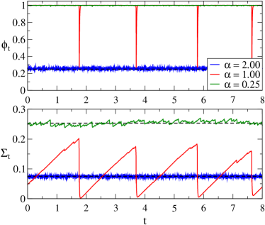
Figure 2: Top: Fraction of jammed elements versus time for a population of $N=10^{4}$ elements undergoing the random walk process described by Eq. (1) (see details in the text). Bottom: corresponding total stress as defined in Eq. (3). Different colors correspond to different values of the coupling constant $\alpha$ (black dashed lines correspond to the analytical stationary solutions in the stable phase). Other parameters are: $\widehat{\gamma}=0.001$, $\widehat{\omega}=15$, $D_{\rm i}=10^{-3}$ , $\mathrm{d}t=10^{-6}$ and $\tau_{\rm pl}=0$.

In order to have a better understanding of the dynamics of the model in the unstable regime it is instructive to look at the empirical probability distribution $P(\sigma,t)$ at different times corresponding to the accelerated build-up of stress and its subsequent relaxation. This is done in Fig. 3 where we plot the empirical $P(\sigma,t)$ at snapshots equally spaced in time (see the caption for details). We observe that initially, $P(\sigma,t)$ is peaked around zero. Then, as some elements become unstable, the stress diffusion constant increases, bringing more elements close to $\sigma_{c}$. This feedback can become explosive and lead to a “spike” in the number of elements that become unstable simultaneously, see Fig. 3, inset.

Finally, since all the calculations above where made assuming $\tau_{\rm pl}=0$, we have explored numerically how the instability behaves when $\tau_{\rm pl}>0$. In this case, we find that the qualitative features of Fig. 1 are left unchanged as long as $\tau_{\rm pl}<\tau_{\rm pl}^{*}$ where the value of $\tau_{\rm pl}^{*}$ depends on other parameters, whereas the instability disappears altogether when $\tau_{\rm pl}>\tau_{\rm pl}^{*}$. For example, in the zero shear rate case, we find for $\widehat{\omega}=30$ and $\alpha=2$ that the instability disappears at $\tau_{\rm pl}^{*}\approx 0.857\ \tau_{\rm fl}$. The reason is quite simple: since jammed elements become unstable at random times with a dispersion $\sim\tau_{\rm pl}$, a large $\tau_{\rm pl}$ maims the synchronisation mechanism that leads to the oscillating instability discovered here. Since the HL model corresponds to $\tau_{\rm pl}/\tau_{\rm fl}\rightarrow\infty$, this oscillating instability would not have shown up in the original HL setting. Note that similarly, a small $\omega$ (corresponding to a large dispersion in the arrival time of the stress signal) is preventing the instability to occur.

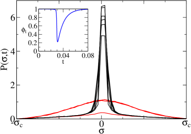
Figure 3: Empirical distribution of stress variables $\sigma_{i}$ for a population of $N=10^{5}$ elements with zero shear rate. Different lines are relative to different snapshots taken at equally spaced time intervals of duration $0.01$ (the corresponding value for the fraction of jammed elements as a function of time is plotted in the inset). Red lines correspond to the build up of the instability (the lower line is at $t=0.03$ for example, approximately corresponding to the minimum of $\phi(t)$ in the inset) while black lines correspond to elements progressively relaxing at $\sigma=0$. For illustrative purposes we set here $\widehat{\gamma}=0$ while other parameters are: $\alpha=1$, $\tau_{\rm fl}=0.01$, $D_{\rm i}=0.01$, $\mathrm{d}t=10^{-6}$, $\widehat{\omega}=30$ and $\tau_{\rm pl}=0$.

VI Conclusion

In this paper, we have revisited the now classic Hébraud-Lequeux model for the rheology of jammed materials. We have argued that a possibly important time scale is missing from HL’s initial specification, namely the characteristic time for a fluidized element to re-jam (chosen to be zero in HL), whose importance has also been stressed in Refs. Coussot and Overlez (2010); Martens et al. (2012); Jagla et al. (2014). A linear stability analysis of the generalized HL model shows that the steady-state solution is in fact unstable for a wide range of parameters, and leads to intermittent, stick-slip flows under a constant shear rate. The stick-slip motion disappears when the shear-rate is large (as expected), or when the time for a jammed element to become unstable is large compared to the re-jamming time, or else when the elastic coupling between jammed elements is either too weak or too strong (see Fig. 1 above).

The instability we find is akin to the synchronization transition of coupled elements that arises in many different contexts (neurons, fireflies, financial bankruptcies, etc.), see Strogatz (2003); Gualdi et al. (2015b) and references therein. Similar instabilities are found in some variants of the SGR models Head, Ajdari and Cates (2001) and within simple phenomenological constitutive equations for shear-thickening materials Aradian and Cates (2006), although the underlying physical mechanism does not seem to be related to the synchronisation effect discussed here. We hope that our scenario could shed light on the commonly observed intermittent, serrated flows of glassy materials under shear. It would also be quite interesting to study our instability in finite dimensions (rather than in the HL mean-field limit), and along the lines recently suggested by Lin and Wyart Lin and Wyart (2015), where the HL diffusion term is replaced by a long-range, Lévy flight diffusion. It is not immediately clear whether the stick-slip instability survives such a deep modification of the mathematical and physical nature of the model.

References

• Baret et al. (2002) J.-C. Baret, D. Vandembroucq, and S. Roux, Phys. Rev. Lett. 89, 195506 (2002).
• Otsuki and Hayakawa (2014) M. Otsuki and H. Hayakawa, Phys.Rev.E 90, 042202 (2014).
• Chen and Bak (1991) K. Chen, P. Bak, and S. Obukhov, Phys. Rev. A 43, 625 (1991).
• Lerner et al. (2012) E. Lerner, G. Düring, and M. Wyart, Europhysics Letters 99, 58003 (2012).
• Argon (1979) A. Argon, Acta Metallurgica 27, 47 (1979).
• Princen (1983) H. Princen, Journal of Colloid and Interface Science 91, 160 (1983).
• Fank and Langer (1998) M. Falk and J. Langer, Phys. Rev. E 57, 7192 (1998).
• Langer (2008) J. Langer, Phys. Rev. E 77, 021502 (2008).
• Schall and Weitz (2007) P. Schall, D. A. Weitz, and F. Spaepen, Science 318, 1895 (2007).
• Manneville et al. (2004) S. Manneville, L. Bécu, and A. Colin, European Physical Journal Applied Physics 28, 361 (2004).
• Amon et al. (2004) A. Amon, V. B. Nguyen, A. Bruand, J. Crassous, and E. Clément, Phys. Rev. Lett. 108, 135502 (2012).
• Maloney and Lemaire (2006) C. E. Maloney and A. Lemaître, Phys. Rev. E 74, 016118 (2006).
• Tanguy et al. (2006) A. Tanguy, F. Leonforte, and J.-L. Barrat, Eur. Phys. J. E 20, 355 (2006).
• Picard et al. (2004) G. Picard, A. Agdari, F. Lequeux, and L. Boquet, Eur. Phys. J. E 15, 371 (2004).
• Hébraud and Lequeux (1998) P. Hébraud and F. Lequeux, Phys. Rev. Lett. 81, 2934 (1998).
• Sollich et al. (1997) P. Sollich, F. Lequeux, P. Hébraud, and M. E. Cates, Phys. Rev. Lett. 78, 2020 (1997).
• Sollich (2006) P. Sollich, in Molecular Gels (Springer, 2006), pp. 161–192.
• Jagla et al. (2014) E. Jagla, F. P. Landes, and A. Rosso, Phys. Rev. Lett. 112, 174301 (2014).
• Lieou et al. (2015) C. K. Lieou, A. E. Elbanna, J. Langer, and J. Carlson, arXiv:1506.00331 (2015).
• Coussot and Overlez (2010) P. Coussot and G. Overlez, Eur. Phys. J. E 33, 183 (2010).
• Rodney et al. (2011) D. Rodney, A. Tanguy, and D. Vandembroucq, Modelling Simul. Mater. Sci. Eng. 19, 083001 (2011).
• Herschel and Bulkley (1926) W. H. Herschel and R. Bulkley, Kolloid-Zeitschrift 39, 291 (1926).
• Agoritsas et al. (2015) E. Agoritsas, E. Bertin, K. Martens, and J.-L. Barrat, Eur. Phys. J. E 38, 71 (2015).
• Jagla (2015) E. Jagla, arXiv:1506.01005 (2015).
• Lin and Wyart (2015) J. Lin and M. Wyart, arXiv:1506.03639 (2015).
• Lemaitre and Caroli (2007) A. Lemaître and C. Caroli, arXiv:0705.3122 (2007).
• Head, Ajdari and Cates (2001) D. A. Head, A. Ajdari, and M. E. Cates, Phys. Rev. E 64, 061509 (2001).
• Aradian and Cates (2006) A. Aradian and M. E. Cates, Phys. Rev. E 73, 041508 (2006).
• Gualdi et al. (2015a) S. Gualdi, M. Tarzia, F. Zamponi, and J.-P. Bouchaud, Journal of Economic Dynamics and Control 50, 29 (2015a).
• Gualdi et al. (2015b) S. Gualdi, J.-P. Bouchaud, G. Cencetti, M. Tarzia, and F. Zamponi, Phys. Rev. Lett. 114, 088701 (2015b).
• Strogatz (2003) S. Strogatz, Sync: The emerging science of spontaneous order (Hyperion, 2003).
• Martens et al. (2012) K. Martens, L. Bocquet, and J.-L. Barrat, Soft Matter 8, 4197 (2012).
• Puosi et al. (2012) F. Puosi, J. Olivier, and K. Martens, arXiv:1501.04574 (2015).