¹²CO emission from EP Aqr: Another example of an axi-symmetric AGB wind?

The CO(1-0) and (2-1) emission of the circumstellar envelope of the Asymptotic Giant Branch (AGB) star EP Aqr has been observed in 2003 using the IRAM Plateau-de-Bure Interferometer and in 2004 using the IRAM 30-m telescope at Pico Veleta. The line profiles reveal the presence of two distinct components centered on the star velocity, a broad component extending up to ${\sim}10$ km s^-1 and a narrow component indicating an expansion velocity of only ${\sim}2$ km s^-1. An early analysis of these data was performed under the assumption of isotropic winds. The present study revisits this interpretation by assuming instead a bipolar outflow nearly aligned with the line of sight. A satisfactory description of the observed flux densities is obtained with a radial expansion velocity increasing from ${\sim}2$ km s^-1 at the equator to ${\sim}10$ km s^-1 near the poles. The mass loss rate is ${\sim}1.8\,10^{-7}$ M_⊙ yr^-1. The angular aperture of the bipolar outflow is ${\sim}45^{\circ}$ with respect to the star axis, which makes an angle of ${\sim}13^{\circ}$ with the line of sight. A detailed study of the CO(1-0) to CO(2-1) flux ratio reveals a significant dependence of the temperature on the star latitude, smaller and steeper at the poles than at the equator at large distances from the star ($>2^{\prime\prime}\equiv 1.0\times 10^{-3}$ pc). Under the hypothesis of radial expansion of the gas and of rotation invariance about the star axis, the effective density has been evaluated in space as a function of star coordinates (longitude, latitude and distance from the star). Evidence is found for an enhancement of the effective density in the northern hemisphere of the star at angular distances in excess of ${\sim}3^{\prime\prime}$ and covering the whole longitudinal range. The peak velocity of the narrow component is observed to vary slightly with position on the sky, a variation consistent with the model and understood as the effect of the inclination of the star axis with respect to the line of sight. This variation is inconsistent with the assumption of a spherical wind and strengthens our interpretation in terms of an axisymmetric outflow. While the phenomenological model presented here reproduces well the general features of the observations, not only qualitatively but also quantitatively, significant differences are also revealed, which would require a better spatial resolution to be properly described and understood.

1 Introduction

EP Aqr is one of the nearest mass losing Asymptotic Giant Branch (AGB) stars (d=114 pc, van Leeuwen 2007), and as such one of the best characterized objects of its class. The absence of Technetium in the spectrum (Lebzelter & Hron 1999), and the low value of the ¹²C/¹³C abundance ratio ($\sim$ 10, Cami et al. 2000) indicate that it is still at the beginning of its evolution on the AGB. Yet Herschel has imaged a large scale ($2^{\prime}\times 4^{\prime}$) circumstellar shell at $$70\text{\,}\mathrm{\SIUnitSymbolMicro}$\mathrm{m}$ (Cox et al. 2012) testifying for a relatively long duration of the mass loss (${>}10^{4}$ years) and for interaction with the surrounding interstellar medium. The elongation of the far-infrared image is in a direction opposite to the EP Aqr space motion. From H i observations at 21 cm, Le Bertre & Gérard (2004) estimate a duration of $\sim$ 1.6$\times$10⁵ years for the present episode of mass loss.

Combined observations have been obtained with the IRAM 30-m telescope and the Plateau-de-Bure Interferometer in ¹²CO(1-0) and ¹²CO(2-1) in 2003 and 2004, improving over earlier observations (Knapp et al. 1998, Nakashima 2006). The spectra, which reveal a wind composed of two main components with expansion velocities ${\sim}2$ and ${\sim}10$ km s^-1, were analyzed in terms of multiple isotropic winds (Winters et al. 2003, 2007). The interferometer data show an extended source of about 15^′′ (FWHM), and evidence for a ring structure in CO(2-1). However, when assuming multiple isotropic winds, Winters et al. (2007) did not manage to fully explain the line profiles obtained at different positions of the spectral maps.

Composite CO line profiles have been observed for several AGB sources, including RS Cnc and X Her (e.g. Knapp et al. 1998). Kahane & Jura (1996) interpreted the narrow line component of X Her in terms of a spherically expanding wind and the broad line component in terms of a bipolar flow, probably observed at a viewing angle of about 15^∘. For RS Cnc, high spatial resolution observations can be interpreted assuming the same geometry but with a different inclination of about 40^∘ with respect to the line of sight (Hoai et al. 2014). These results raise the question whether the bipolar outflow hypothesis might also apply to EP Aqr.

The present study is therefore revisiting the analysis of Winters et al. (2007), assuming instead a bipolar outflow approximately directed along the line of sight. We exploit the experience gained in similar studies of other stars, RS Cnc (Hoai et al. 2014, Nhung et al. 2015) and the Red Rectangle, a post-AGB source, which could be interpreted by applying a similar model (Tuan Anh et al. 2015).

The paper is organised as follows: in Sect. 2 we present reprocessed data on EP Aqr that will be used in this work. Sect. 3 describes in an elementary way the main features implied by the assumed orientation of EP Aqr, with the star axis nearly parallel to the line of sight, mimicking spherical symmetry. Sect. 4 presents an analysis of the data using a simple bipolar outflow model that had been developed earlier for RS Cnc (Hoai et al. 2014, Nhung et al. 2015); the results of the best fit to the observations is used as a reference in the following sections. Sect. 5 presents a study of the CO(1-0) to CO(2-1) emission ratio, allowing for an evaluation of the temperature distribution nearly independent of the model adopted for the description of the gas density and velocity. Sect. 6 uses the distribution of the gas velocity obtained in Sect. 4 to reconstruct directly in space the effective gas density, without making direct use of the parametrization of the flux of matter obtained in Sect. 4, and providing therefore a consistency check of the results of the model. Finally, Sect. 7 presents a detailed study of the spatial variation of the radial velocity of the narrow line component. It provides a sensitive check of the bipolar outflow hypothesis and of its small inclination angle with respect to the line of sight.

2 Observations

The observations analysed here combine interferometer data obtained using the Plateau-de-Bure Interferometer with short-spacing data obtained using the Pico Veleta 30-m telescope. A detailed description of the original observations is given in Winters et al. (2007). ¹²CO(2-1) and ¹²CO(1-0) spectral data have been obtained with a spatial resolution of ${\sim}1^{\prime\prime}$ and ${\sim}2^{\prime\prime}$ respectively and a spectral resolution of 0.1 km s^-1. At such spatial resolution, the two spectral components present in the single-dish line spectra are seen as originating from the same region. The images are virtually circularly symmetric and display smooth variations with velocity and projected distance from the star. In Winters et al. (2007) the observed spectra were interpreted by a succession of spherically symmetric and short-spaced mass-loss events. These authors noted the presence of inhomogeneities in the spectral maps indicating a possible clumpiness of the circumstellar envelope.

We have reprocessed the original data, correcting for an artifact introduced by a velocity shift of 0.52 km s^-1 in the CO(1-0) data and recentering the maps on the position of the star at epoch 2004.0, correcting for its proper motion as determined by van Leeuwen (2007). The reprocessed channel maps are shown in Figs. 1 and 2.

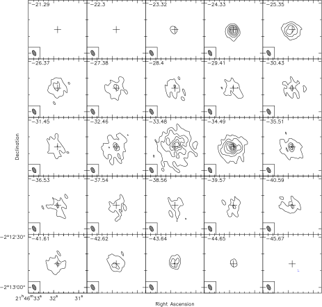
Figure 1: Channel maps in the ¹²CO(J=1-0) line (smoothed to a width of 1 km s^-1). Contours are plotted at 5, 10, 20, 30, 40 $\sigma$ (1 $\sigma=14\,$mJy/beam). The synthesized beam is indicated in the lower left.

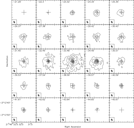
Figure 2: Channel maps in the ¹²CO(J=2-1) line (smoothed to a width of 1 km s^-1). First contour is plotted at 10 $\sigma$, the following contours start at 20 $\sigma$ and are plotted in 20 $\sigma$ steps (1 $\sigma=16\,$mJy/beam). The synthesized beam is indicated in the lower left.

3 Observing a star along its symmetry axis

The high degree of azimuthal symmetry observed in the channel maps of both CO(1-0) and CO(2-1) emission (see Figs. 1 and 2, Winters et al. (2007)) implies that a bipolar outflow, if present, should have its axis nearly parallel to the line of sight. In such a configuration, some simple relations apply between the space coordinates and their projection on the sky plane. We review them briefly in order to ease further discussion. We use coordinates (Fig. 3) centered on the star with $x$ along the star axis, parallel to the line of sight, $y$ pointing east and $z$ pointing north. We assume rotation symmetry about the $x$ axis and symmetry about the equatorial $(y,z)$ plane of the star. Defining $\rho$ the gas density, $T$ the gas temperature and $\boldsymbol{V}$ the gas velocity in the star rest frame, having components $V_{x}$, $V_{y}$, $V_{z}$, the following relations apply at point $(x,y,z)$: $\rho$ and $T$ are functions of $r=(x^{2}+y^{2}+z^{2})^{\frac{1}{2}}$ and of $|\alpha|$ where $\alpha=arctan(x/R)$ is the latitude in the star reference system, and $R=(y^{2}+z^{2})^{\frac{1}{2}}$ is the projection of $r$ on the sky plane.
The velocity $\boldsymbol{V}$ takes a simple form when expressed in terms of meridian coordinates, $R=y\cos\omega+z\sin\omega$, $x$ and $\eta=-y\sin\omega+z\cos\omega$, $\omega$ being the star longitude; its components are then functions of $r$ and $|\alpha|$. In case of pure radial expansion, $V_{\eta}=0$, $V_{x}=xV/r$ and $V_{R}=RV/r$ while in case of pure rotation $V_{R}=V_{x}=0$.

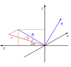
Figure 3: Definition of coordinates. The $(y,z)$ coordinates are obtained by rotation of angle $\omega$ in the sky plane about the $x$ axis (line of sight and star axis, cf. Sect. 3). In the sky plane, y is towards East, and z towards North.

In the case of pure radial expansion with a known radial dependence of the velocity, the flux density $f$ measured in a pixel $(y,z)$ at velocity $V_{x}$ is associated with a well defined position in space, obtained from

$$x=rV_{x}/V=(x^{2}+R^{2})^{\frac{1}{2}}V_{x}/V=RV_{x}(V^{2}-V_{x}^{2})^{-\frac{1}{2}}.$$ (1)

Then, if one knows $V$, one can calculate $V_{x}$ and therefore its derivative $dV_{x}/dx$ at any point in space. Defining an effective density $\rho_{\mathrm{eff}}$ as $\rho_{\mathrm{eff}}=fdV_{x}/dx$, such that the observed flux in a given pixel be $\int{fdV_{x}}=\int{\rho_{\mathrm{eff}}dx}$, one is then able to calculate it at any point in space. The effective density, defined by this relation, is the product of the actual gas density and a factor accounting for the population of the emitting state, the emission probability and correcting for the effect of absorption.

We illustrate the above properties with a simple example, close to the reality of EP Aqr. We assume exact rotation invariance about the star axis (parallel to the line of sight), a purely radial wind with a velocity that only depends on $\alpha$

$$V=V_{0}+V_{1}\sin^{2}\!\alpha$$ (2)

($V_{0}$ at the equator and $V_{0}+V_{1}$ at the poles) and an effective density (defined such that its integral over the line of sight measures the observed flux density) inversely proportional to $r^{2}$. From $V_{x}=V\sin\alpha$ and Eq. (2) we obtain $\sin^{3}\!\alpha+(V_{0}/V_{1})\sin\alpha-(V_{x}/V_{1})=0$. This reduced cubic equation is explicitly solvable with $\sin\alpha=-(q-s)^{\frac{1}{3}}-(q+s)^{\frac{1}{3}}$, $s=(q^{2}+p^{3})^{\frac{1}{2}}$, $p=\frac{1}{3}V_{0}/V_{1}$ and $q=-\frac{1}{2}V_{x}/V_{1}$. For a given value of the Doppler velocity $V_{x}$ one can therefore calculate $\alpha$ independent of $R$: in any pixel, $V_{x}$ and $\alpha$ are related in the same way, which is illustrated in Fig. 4 (upper panel). Similarly, $V_{x}$ and $r/R=1/\cos\alpha$ are also related in a universal way, independent of $R$ (Fig. 4, middle panel). The resulting velocity spectra are displayed in Fig. 4 (lower panel) for $R$=1, 2, 3, 4 and 5 (all quantities are in arbitrary units except for the velocities that are in km s^-1 with $V_{0}=2$ km s^-1 and $V_{1}=8$ km s^-1). They simply scale as $1/R$, reflecting the $1/r^{2}$ dependence of the effective density. In such a simple model, the flux ratio between the CO(1-0) and CO(2-1) is a constant, independent of $R$ and $V_{x}$.

Figure 4: Relation between the Doppler velocity $V_{x}$ and the star latitude $\alpha$ (cf. Eq. (2), upper panel), the ratio $r/R=1/cos\alpha$ (middle panel) for the simple star model described in the text. Lower panel: velocity spectra obtained for the same model at $R$=1, 2, 3, 4 and 5 (running downward).

4 Comparison of the observations with a bipolar outflow model

The spectral maps extracted from the reprocessed data (see Sect. 2) are shown in Fig. 5. The spectra are displayed in steps of 1^′′ in right ascension and declination. The synthesized beam is $3.53^{\prime\prime}\times 1.84^{\prime\prime}$ (PA=28^∘) for CO(1-0), and $1.67^{\prime\prime}\times 0.94^{\prime\prime}$ (PA=29^∘) for CO(2-1), respectively.

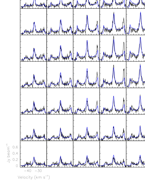
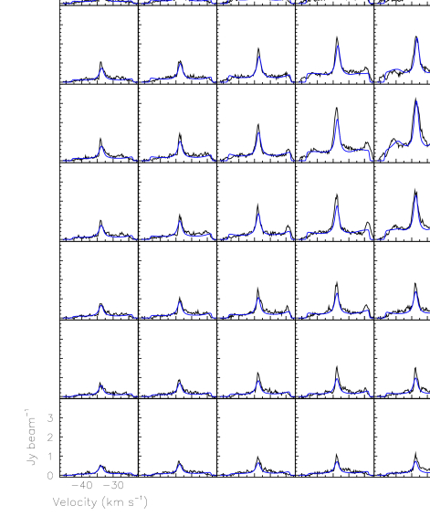
Figure 5: Spectral maps centered on the star of the CO observations (black) and the best-fit model (blue). The CO(1-0) map is shown in the upper panel, CO(2-1) in the lower panel. Steps in right ascension and declination are $1^{\prime\prime}$.

To describe EP Aqr, we use the model of Hoai et al. (2014), which assumes that the wind is purely radial, free of turbulence, and in local thermal equilibrium. For solving the radiative transfer, a ray-tracing method that takes absorption into account is used (Hoai 2015). Moreover, the wind is assumed to be stationary and is supposed to have been in such a regime for long enough a time, such that the radial extension of the gas volume is governed exclusively by the UV dissociation of the CO molecules by interstellar radiation (Mamon et al. 1988) and does not keep any trace of the star history. For EP Aqr the CO/H abundance ratio is taken as 2.5 $10^{-4}$ (Knapp et al. 1998), a value representative for an M-type star. The temperature is parametrized by a power law of $r$, $T=T_{0}r^{-n}$ but is independent of the stellar latitude $\alpha$. The spectrum of flux densities in each pixel is calculated by integration along the line of sight, the temperature dependent contributions of emission and absorption being respectively added and subtracted at each step. The wind velocity $V$ and the flux of matter $f_{M}$ are smooth functions of $|\sin\alpha|$ and allowance is made for a radial velocity gradient described by parameters $\lambda_{1}$ at the poles and $\lambda_{2}$ at the equator. Assuming the wind to be stationary, the density $\rho$ is then defined at any point by the relation $\dot{M}(\alpha)=4\pi f_{M}(\alpha)=4\pi r^{2}\rho(\alpha,r)V(\alpha,r)=const(\alpha)$.

The bipolarity of the flow is parametrized as a function of $\sin\alpha$ using Gaussian forms centered at the poles:

$$G=exp[-\frac{1}{2}(\sin\alpha-1)^{2}/\sigma^{2}]+exp[-\frac{1}{2}(\sin\alpha+1)^{2}/\sigma^{2}],$$ (3)

where $\sigma$ is a parameter to be adjusted. This function is used to define the $\sin\alpha$ dependence of both the wind velocity and the flux of matter:

$$V=V_{1}G(1-\lambda_{1}e^{-r/2.5^{\prime\prime}})+V_{2}(1-\lambda_{2}e^{-r/2.5^{\prime\prime}})$$ (4)

and

$$f_{M}=f_{M_{1}}G+f_{M_{2}}.$$ (5)

The density then results from mass conservation:

$$\rho=r^{-2}(f_{M_{1}}G+f_{M_{2}})/[V_{1}G(1-\lambda_{1}e^{-r/2.5^{\prime\prime}})+V_{2}(1-\lambda_{2}e^{-r/2.5^{\prime\prime}})].$$ (6)

For $r$-independent wind velocities, $\lambda_{1}=\lambda_{2}=0$, the velocity and flux of matter are nearly $V_{1}+V_{2}$ and $f_{M_{1}}+f_{M_{2}}$ at the poles and $\varepsilon V_{1}+V_{2}$ and $\varepsilon f_{M_{1}}+f_{M_{2}}$ at the equator where $\varepsilon$ is the small positive value taken by $G$ at the equator.

A small inclination $\theta$ of the star axis with respect to the line of sight, with position angle $\psi$ with respect to the north, is made allowance for. The relations quoted in Sect. 3 for $\theta=0$ are modified accordingly. More precisely, the position of the star frame with respect to the sky plane and line of sight is now defined by angles $\theta$ and $\psi$ and the polar coordinates in the star frame are the latitude $\alpha$ and the longitude $\omega$ defined in such a way as to conform with the definition given in Sect. 3 for $\theta=0$. The star radial velocity as determined from the CO line profiles is $-33.5$ km s^-1 in good agreement with the value of $-34$ km s^-1 derived in Winters et al. (2003). The values taken by the parameters are obtained by a standard $\chi^{2}$ minimization method. The best fit values of the parameters of the model to the joint CO(1-0) and CO(2-1) observations are listed in Table 1 and the quality of the fit is illustrated in Fig. 5 where modeled velocity spectra are superimposed over observed ones.

Table 1: Best fit parameters obtained for the CO(1-0) and CO(2-1) data. A distance of 114 pc is adopted.

Parameter	Best fit value
$\theta$	13∘
$\psi$	144∘
$\sigma$	0.3
$V_{1}$	8.0 km s-1
$V_{2}$	2.0 km s-1
$f_{M_{1}}$	1.26 10-8 M⊙ yr-1sr-1
$f_{M_{2}}$	0.49 10-8 M⊙ yr-1sr-1
$\lambda_{1}$	0.52
$\lambda_{2}$	0.38
$T_{0}$ ($r=1^{\prime\prime}$)	116 K
$n$	0.77

This result shows that it is possible to describe the morphology and kinematics of the gas envelope of EP Aqr as the combination of a slow isotropic wind and a bipolar outflow, the wind velocities at the equator and at the poles being ${\sim}2\,$km s^-1 and ${\sim}10\,$km s^-1 respectively and the inclination of the star axis with respect to the line of sight, $\theta$, being ${\sim}13^{\circ}$. The flux of matter varies from 0.49 10^-8 M_⊙ yr^-1sr^-1 in the equatorial plane to 1.26 10^-8 M_⊙ yr^-1sr^-1 in the polar directions. The total mass loss rate (integral of $\dot{M}(\alpha)$ over $\alpha$) is 1.8 10^-7 M_⊙ yr^-1. The angular aperture of the bipolar outflow, measured by the parameter $\sigma=0.3$ in Eq. (3), corresponds to $\alpha=\arcsin(0.7)\sim 45^{\circ}$.

Leaving for Sect. 7 a more detailed discussion of this result, we study in the next section the CO(1-0) to CO(2-1) flux ratio, which gives important information on the temperature distribution with only minimal dependence on the details of the model.

5 The CO(1-0) to CO(2-1) flux ratio

Comparing the fluxes associated with CO(1-0) and CO(2-1) emission provides information on the gas temperature nearly independently from the gas density and velocity, which are common to the two lines. In the optically thin limit and assuming local thermal equilibrium, the temperature $T$(K) is obtained from the ratio $Q$ of the CO(1-0) to CO(2-1) fluxes as $T=11.1/\ln(Q/0.063)$. However, the model presented in the preceding section does not reproduce well the observed flux ratio. In particular, we observe that $Q$ is sometimes below the minimal value 0.063 allowed by the local thermal equilibrium hypothesis (when $T=\infty$). This is illustrated in Fig. 6, where the data have been averaged over concentric rings limited by circles having $R$=1^′′, 2^′′, 3^′′, 4^′′ and 5^′′ respectively.

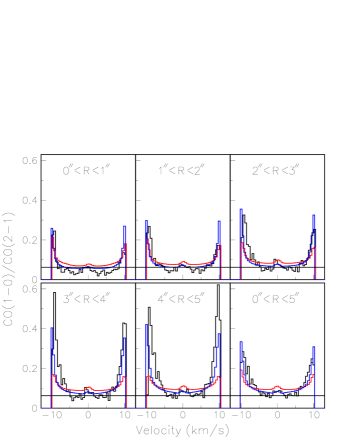
Figure 6: CO(1-0) to CO(2-1) flux ratio (black) where each of the CO(1-0) and CO(2-1) fluxes has been averaged over 5 successive velocity bins and over the concentric rings defined in the text. The lower right panel is for all pixels having $R<5^{\prime\prime}$. The result of the best fit of the model described in Sect. 4 is shown in red and that of its modification described in Sect. 5 is shown in blue. The horizontal lines indicate the level (0.063) above which the data must be under the hypothesis of local thermal equilibrium.

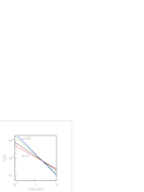
Figure 7: Distribution of the gas temperature. Left: as a function of $\alpha$ at distances from the star $r=1^{\prime\prime}$ to $8^{\prime\prime}$ (from top to bottom) in steps of $1^{\prime\prime}$; right: as a function of $r$ at latitudes $\alpha=0^{\circ}$ (red), $30^{\circ}$ (black), $60^{\circ}$ (green) and $90^{\circ}$ (blue).

Accordingly, we allow for a small difference of normalization between the CO(1-0) and CO(2-1) fluxes by multiplying the former by a factor $1+\mu$ and the latter by a factor $1-\mu$. This factor may account for a real difference in calibration as well as, in an ad hoc way, for any inadequacy of the model (assumption of local thermal equilibrium, absence of turbulence). Moreover, we see from Fig. 6 that one needs to increase the ratio $Q$ near the extremities of the velocity spectrum more than in the middle, meaning near the poles at large values of $r$ more than near the equator at small values of $r$. Accordingly, we parametrize the temperature in the form

$$T=T_{0}(\sin^{2}\!\alpha+a\cos^{2}\!\alpha)(r/1^{\prime\prime})^{-n}$$ (7)

with

$$n=n_{1}+n_{2}\cos^{2}\!\alpha.$$ (8)

At $r=1^{\prime\prime}$, the temperature is $T_{0}$ at the poles and $aT_{0}$ at the equator. The power index describing the radial dependence of the temperature is $n_{1}$ at the poles and $n_{1}+n_{2}$ at the equator.

The result is summarized in Table 2 and illustrated in Fig. 7. The ratio between the values taken by the temperature at the equator and at the poles, $ar^{-n_{2}}$, varies from 0.70 at $r=1^{\prime\prime}$ to 1.64 at $r=5^{\prime\prime}$, crossing unity at $r\approx 2^{\prime\prime}$. As $r/R$ is much larger near the poles than at the equator (it is equal to 1/cos$\alpha$ in the simple configuration studied in Sect. 3), the extremities of the velocity spectrum probe large $r$ values, meaning low temperatures, as required by the measured $Q$ values: both the values taken by $n_{2}$ and by $a$ are determinant in increasing $Q$ at the extremities of the velocity spectrum. For the same reason, the temperature increase obtained from the parametrization at small values of $r$ and large values of $\alpha$ is not probed by any of the data, which makes its reliability uncertain.

The values of the temperature that we find close to the central star ($\sim$ 1000 K at 0.1^′′) are consistent with those obtained by Cami et al. (2000) using infrared CO₂ lines.

Table 2: Best fit parameters of the CO(2-1) to CO(1-0) ratio.

Parameter	$T_{0}$(K)	a	$n_{1}$	$n_{2}$	$\mu$ (%)	$\chi^{2}/dof$
Best fit values	170	0.67	1.22	$-$0.55	9.0	1.14
Uncertainties	20	0.12	0.06	0.10	3.0

The uncertainties listed in Table 2 are evaluated from the dependence of $\chi^{2}$ over the values of the parameters, taking proper account of the correlations between them. However, they have been scaled up by a common factor such that the uncertainty on $T_{0}$ be 20 K. This somewhat arbitrary scaling is meant to cope with our lack of detailed control over systematic errors and the value of 20 K is evaluated from the robustness of the results against changes of different nature that have been made to the model finally adopted in the course of the study. While the quoted uncertainties give a good idea of the reliability of the result and of its sensitivity to the values taken by the parameters, both the quality of the data (in particular the need for a $\mu$-correction) and the crudeness of the model do not allow for a more serious quantitative evaluation.

We noted that the quality of the fits can be slightly improved by allowing for a temperature enhancement at mid-latitudes and small distances to the star; however, we were unable to establish the significance of this result with sufficient confidence.

The following two conclusions can then be retained:

• At large distances to the star, the temperature is significantly higher at the equator than at the poles, by typically 15 K at $r=5^{\prime\prime}$;

• The temperature decreases with distance as ${\sim}r^{-1.2}$ at the poles and significantly less steeply at the equator, typically as $r^{-0.7}$.

6 Evaluation of the effective density in the star meridian plane

Under the hypotheses used to evaluate the model described in Sect. 4, one can associate to each data-triple $(y,z,V_{x})$ a point $(r,\alpha)$ in the meridian plane of the star. Indeed, $x$ is a known function of $r$, $\alpha$, and the star longitude $\omega$, as is $V_{x}=Vx/r$. The former uses the values of $\theta$ and $\psi$ and the latter the parametrization of $V$ as a function of $r$ and $\alpha$ that were obtained from the best fit. As one has three equations and three unknowns one obtains $r$, $\alpha$ and $\omega$ given $V_{x}$, $y$ and $z$. The flux density $f$ corresponding to a given data-triple can therefore be mapped as an effective density $\rho_{\mathrm{eff}}=f\mathrm{d}V_{x}/\mathrm{d}x$ in the meridian plane of the star, (i.e. each plane that contains the star’s polar axis) with coordinates $r\cos\,\alpha$ and $r\sin\,\alpha$ (see Fig. 3). Its evaluation uses the best fit parametrization of the wind velocity but not that of the flux of matter: it provides therefore a consistency check.

The validity of the procedure has been checked by replacing the data by the results of the model and verifying that the reconstructed effective density is identical to that used as input. The region of large $|\alpha|$ values is probed exclusively by the central pixels near the extremity of the spectrum and is therefore subject to large systematic uncertainties. Indeed, large $|\alpha|$ values mean large $|V_{x}|$ values, which in turn mean large $r/R$ values, namely $R$ much smaller than $r$. For this reason, on the basis of the result of the validity check, we restrict the space reconstruction to pixels having $R>1^{\prime\prime}$. In addition, in order to avoid dealing with too low fluxes, we require $R$ not to exceed 10^′′. The resulting maps of $r^{2}\rho_{\mathrm{eff}}$ are displayed in Fig. 8 for CO(1-0) and CO(2-1) separately and its averaged distributions as functions of $r$, $\alpha$ and $\omega$ in Fig. 9.

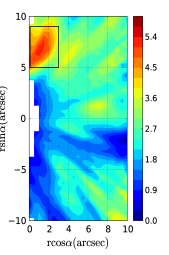
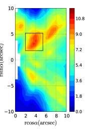
Figure 8: Reconstructed maps of the effective density, multiplied by $r^{2}$, in the star meridian plane under the assumption of a wind velocity having the form obtained from the best fit of the model of Sect. 4. The colour codes are such that the ratio between maximum and minimum values of $\rho r^{2}$ are the same for CO(1-0) (left) and CO(2-1) (right). Units are Jy beam^-1 km s^-1 arcsec. The rectangles show the regions selected for displaying the $\omega$ distributions shown in Fig. 10 (for CO(1-0), abscissa between $0^{\prime\prime}$ and $3^{\prime\prime}$, ordinate between $5^{\prime\prime}$ and $9^{\prime\prime}$; for CO(2-1), abscissa between $2.0^{\prime\prime}$ and $5.4^{\prime\prime}$, ordinate between $1.8^{\prime\prime}$ and $5.2^{\prime\prime}$).

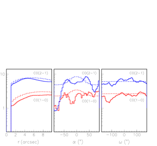
Figure 9: Distributions of the average effective density, multiplied by $r^{2}$, reconstructed in the meridian plane of the star for a wind velocity having the form obtained from the best fit of the model of Sect. 4. Note that the $\mu$-correction has not been applied. left: radial dependence of $r^{2}\rho_{\mathrm{eff}}$, averaged over $\alpha$ and $\omega$; middle: latitude dependence of $r^{2}\rho_{\mathrm{eff}}$, averaged over $r$ and $\omega$; right: longitude dependence of $r^{2}\rho_{\mathrm{eff}}$, averaged over $r$ and $\alpha$. In each panel, CO(1-0) results are shown in red and CO(2-1) results in blue. The dashed curves show the results of the model, ignoring absorption.

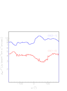
Figure 10: Distributions of the effective density, multiplied by $r^{2}$, as a function of star longitude $\omega$ for the annular regions delineated by the rectangles shown in Fig. 8. CO(1-0) data are shown in red, CO(2-1) data in blue.

All distributions display significant deviations with respect to the distributions generated by the model, which, however, reproduces well the general trends. In principle, one should be able to include in the model the result of the space reconstruction of $\rho_{\mathrm{eff}}$ and iterate the fitting procedure with a more realistic parametrization of the flux of matter and possibly a more sophisticated velocity model. However, the quality of the present data is insufficient to undertake such an ambitious programme. We shall be satisfied with simply taking note of the differences between the model of Sect. 4 and the image revealed by the space reconstruction, as long as they can be considered as being both reliable and significant.

The maps of Fig. 8 and the $\alpha$ distributions of Fig. 9 give evidence for a significant asymmetry between the northern and southern hemispheres of the star (defining north and south in the star coordinate system, north corresponding to $\alpha=\pi/2$, away from Earth, with a projection towards North in the sky plane). Indeed, a modification of the model allowing for an asymmetry of the same form as used in Nhung et al. (2015) for RS Cnc, namely multiplying the flux of matter by a common factor $1+\gamma\sin\alpha$, gives a 20% excess in the northern hemisphere of the star. Differentiating between the asymmetries of the two mass loss terms, $f_{M_{1}}G$ and $f_{M_{2}}$ reveals a strong correlation between them, the asymmetry of the first term being more efficient at improving the quality of the fit. Restricting the asymmetry to the first term results in a 37% excess in the northern hemisphere. The effect of absorption does not exceed ${\sim}5$% on average and cannot be invoked to explain such asymmetry. The fluctuations observed in the distributions of the effective density, as well as the differences observed between the CO(1-0) and CO(2-1) data, make it difficult to locate precisely the northern excess in space. Fig. 10 displays the $\omega$ distributions of the effective density averaged over the $r$-$\alpha$ rectangles drawn in Fig. 8 around the maxima of the meridian maps; they do not show an obvious enhancement, the maximum observed in CO(2-1) corresponding in fact to a minimum in CO(1-0). This suggests that the northern excess is distributed over the whole range of star longitudes rather than being confined to a particular region in space. This is confirmed by the $(y,z)$ sky maps of the measured fluxes (integrated over Doppler velocity and multiplied by $R$) that are displayed in Fig. 11 and show an enhancement at radii exceeding ${\sim}3^{\prime\prime}$. This enhancement, which was already noted by Winters et al. (2007) in the case of the narrow velocity component for CO(2-1), is also visible in the broad velocity component. A better space resolution would be necessary to make more quantitative statements concerning this excess, its precise location, morphology and velocity distribution. The present data allow for a qualitative description, retaining as likely the presence of a northern enhancement at distances from the star exceeding $3^{\prime\prime}$ and distributed more or less uniformly in star longitude.

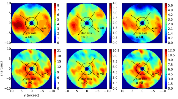
Figure 11: Sky maps of $Rf$ for CO(1-0) (upper panels) and CO(2-1) (lower panels) observations. Units are Jy beam^-1 km s^-1 arcsec. From left to right: all velocities, $|V_{x}|<2$ km s^-1 and $|V_{x}|>2$ km s^-1. The circles at $R=3.5^{\prime\prime}$ correspond to the enhancement seen by Winters et al. (2007) in CO(2-1) data restricted to the narrow velocity component. The projection of the star axis on the sky plane (making an angle of $13^{\circ}$ with the line of sight) and the axis from which the star longitude $\omega$ is measured (positive clockwise) are shown as black arrows.

7 The mean Doppler velocity of the narrow line component

The centroid of the narrow component of the observed spectra moves across the sky map by ${\sim}\pm 0.5$ km s^-1 on either side of the average velocity. We measure its mean velocity $\Delta v$ in each pixel after subtraction of the underlying broad component, interpolated from control regions spanning velocity intervals between 5.4 km s^-1 and 2.6 km s^-1 with respect to the average velocity (either blue-shifted or red-shifted). The procedure is illustrated in Fig. 12 for the spectra summed over the 37$\times$37=1369 pixels of the sky map $(9.25^{\prime\prime}\times 9.25^{\prime\prime})$. The resulting $\Delta v$ distributions, measured in km s^-1 with respect to the mean velocity measured for the whole maps, are shown in Fig. 13 (left) and their maps in Fig. 14. Both CO(1-0) and CO(2-1) data display very similar features, the narrow component being seen to be red-shifted in the north-west direction and blue-shifted in the south-east direction, nearly parallel to the direction of the projected star axis. This suggests that the inclination of the star axis with respect to the line of sight, measured by the angle $\theta{\sim}13^{\circ}$, might be the cause of the effect.

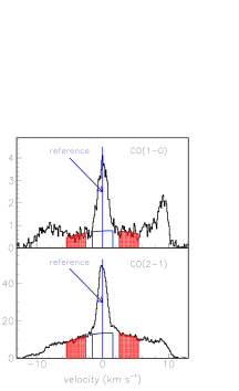
Figure 12: Illustration of the procedure used to evaluate the mean Doppler velocity $\Delta v$ of the narrow component. The velocity spectra summed over the 1369 pixels of the map are shown in black for CO(1-0) (upper panel) and CO(2-1) (lower panel). The quadratic fit over the two control regions is shown in red and its interpolation below the narrow component in blue. The vertical blue lines show the mean Doppler velocities of the narrow component from which the interpolated broad component has been subtracted. They are used as reference for evaluating $\Delta v$ in each pixel separately.

In order to assess quantitatively the validity of this interpretation, we define a band running from south-east to north-west as shown in Fig. 14. Calling $\xi$ the sky coordinate running along the band, we display in Fig. 13 (right) the dependence of $\Delta v$ on $\xi$ for pixels contained inside the band. It reveals a complex structure with successive bumps superimposed over a global increase, displaying remarkable similarities between CO(1-0) and CO(2-1), implying that it is likely to be real rather than an artifact of the analysis or instrumental. As a model, we use the best fit introduced in Sect. 4, however with the temperature distribution and the adjustment of the relative CO(1-0) to CO(2-1) normalization that were introduced in Sect. 5. As illustrated in Figs. 15 and 16, the adopted model reproduces correctly the main features of the observed distributions: the width of the $\Delta v$ distribution and the amplitude of the Doppler shift when moving from south-east to north-west along the $\xi$ axis. Again, as in the preceding section, observations are well reproduced by the model, not only qualitatively but also quantitatively in their general features. This is only achieved by the hypothesis of a bipolar wind structure and is inconsistent with the assumption of a spherical outflow.

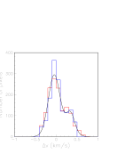
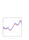
Figure 13: Left: distributions of the mean Doppler velocity $\Delta v$ (km s^-1) measured with respect to its value averaged over the whole map (shown as ”reference” in Fig. 12). The black curve shows a two-Gaussian common fit to the two distributions. Right: dependence of the projection of the mean Doppler velocity $\Delta v$ (km s^-1), averaged over pixels included in the bands shown in Fig. 14, on coordinate $\xi$ measured from south-east to north-west. The black curve shows a polynomial common fit to the two distributions. In both panels the CO(1-0) data are shown in red and the CO(2-1) data in blue.

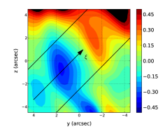
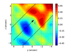
Figure 14: Sky maps of the mean Doppler velocity $\Delta v$ (km s^-1) measured with respect to its value averaged over the whole map (shown as ”reference” in Fig. 12) for CO(1-0) (left) and CO(2-1) (right). The black lines limit the bands in which pixels are retained to evaluate the $\xi$ dependence of $\Delta v$ (Fig. 13 right).

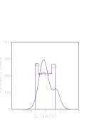
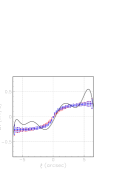
Figure 15: Results of the model introduced in Sect. 4 for the distributions displayed in Fig. 13. The smooth curves are the results of the fits (respectively Gaussian and polynomial) made to the observations in Fig. 13.

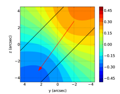
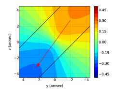
Figure 16: Results of the model introduced in Sect. 4 for the maps displayed in Fig. 14. The red arrows indicate the projection of the star axis on the sky plane.

8 Discussion

Applying a bipolar outflow model to analyze the spatially resolved CO(1-0) and CO(2-1) spectra from EP Aqr results in an excellent agreement of the model results with the observations. The peculiar geometry of the star orientation, with the symmetry axis nearly parallel to the line of sight, implies an approximate circular symmetry when projected on the sky and gives the illusion of a spherically symmetric gas distribution. However, when correlated with the Doppler velocity distributions, it allows for a transparent interpretation in terms of the spatial effective density, each data-triple being associated with a single point in space once the velocity of the radial wind is known. Under the hypotheses of pure radial expansion and of rotation invariance about the star axis, it is possible to reconstruct the space distribution of the effective density. As a first step, we have compared the observations with a simple bipolar outflow model that had been developed earlier to describe another AGB star, RS Cnc. A satisfactory description has been obtained by adjusting the model parameters to best fit the CO(1-0) and CO(2-1) data together. Several parameters defining the morphology and the kinematics of the gas volume surrounding EP Aqr have been evaluated this way with good confidence. Among these are the orientation of the star axis, making an angle of ${\sim}13^{\circ}$ with the line of sight and projected on the sky plane at ${\sim}144^{\circ}$ from north toward west. The velocity of the radial wind has been found to increase from ${\sim}$2 km s^-1 at the star equator to ${\sim}$10 km s^-1 at the poles. The flux of matter is also enhanced at the poles, however less than the radial wind, resulting in an effective density slightly enhanced in the equator region. This shows that an axi-symmetry such as that observed in EP Aqr (or RS Cnc, see figure 6 in Hoai et al. 2014) is more clearly revealed by velocity-resolved data. For instance infrared data obtained in the continuum, even at very high spatial resolution, could not reveal such an effect. Such a kind of morpho-kinematics could explain that asymmetries in AGB outflows are found preferentially through radio observations obtained at high spectral resolution (e.g. Castro-Carrizo et al. 2010). However, this characteristic of the model is partly arbitrary and its main justification is to give a good description of the observations. We do not claim that the form adopted in the proposed model is unique; on the contrary we are confident that other forms could have been chosen with similar success. In particular, the hypothesis of pure radial expansion retained in the model should not be taken as evidence for the absence of rotation of the gas volume about the star axis. Indeed, such rotation, if it were present, would be virtually undetectable as the resulting velocities, being nearly perpendicular to the line of sight, would not produce any significant Doppler shift.

The assumptions made in formulating the model are always approximations, some time very crude, of the reality. In particular, evidence has been obtained for significant departures from the symmetry with respect to the star equatorial plane assumed in the model, revealing an excess of emission at northern star latitudes over the whole longitudinal range at angular distances from the star exceeding ${\sim}3^{\prime\prime}$. This feature, at least part of it, had already been noted earlier (Winters et al. 2007) and thought to suggest the existence of successive mass loss events. In other words a succession of mass loss events can be mimicked by a latitudinal variation of the flux of matter.

In general, while the proposed model has been very efficient at describing the main features and general trends of the flux densities, some significant deviations with respect to the observations have also been found. The present data, in particular their spatial resolution, prevent a more detailed statement about the nature of these deviations. An important asset of the model is to illustrate the efficiency of the method used to reconstruct the spatial morphology and kinematics of the gas envelope. Once data of a significantly better resolution will be available, e.g. from ALMA, using the same methodology will reveal many of such details with unprecedented reliability and precision.

The availability of measurements of the emission of two different rotation lines of the same gas is extremely precious and has been exploited as much as possible, based on the current data. The flux ratio of two lines allows to evaluate the temperature distribution of the gas in a region where the ratio between the populations and emission probabilities of the two states vary rapidly, which is the case for angular distances from the star probed by the present observations. Most of the details of the model are irrelevant to the value of the flux density ratio between the two lines, which depends mostly on temperature under reasonable approximations (local thermal equilibrium, absence of large turbulence, etc.). Through this property, evidence was found for a significant enhancement of temperature at the star equator, therefore correlated with the orientation of the bipolar flow and at variance with the hypothesis of a pure radial dependence.

A method allowing iterating the wind velocity and the effective density in successive steps has been sketched. When data with significantly improved spatial resolution will be available, this will provide a very efficient analysis tool. The peculiar orientation of EP Aqr makes such an analysis much more transparent than in the general case where the star axis is neither parallel nor perpendicular to the sky plane.

Furthermore, the good spectral resolution of the present observations has made it possible to finely analyse the variations of the Doppler velocity of the narrow line component across the sky map, providing a sensitive test of the validity of the bipolar flow hypothesis and a quantitative check of the inclination of the star axis with respect to the line of sight.

The present work leads us to prefer a bipolar, stationary, wind model over the spherical, variable, scenario that was proposed earlier. AGB stars have traditionally been assumed to be surrounded by almost spherical circumstellar shells. Deviations, sometimes spectacular, from spherical symmetry are observed in planetary nebulae (PNs). Such deviations are also observed in post-AGB sources and it is generally considered that they arise during the phase of intense mass loss, after the central stars have evolved away from the AGB. However, it has also been recognized that the geometry of circumstellar shells around AGB stars may sometimes show an axi-symmetry (e.g. X Her, Kahane & Jura (1996); RS Cnc, Hoai et al. (2014)). The origin of this axi-symmetry has not been clearly identified: magnetic field, stellar rotation, or presence of a close binary companion may play a role. Recently, Kervella et al. (2015) reported the detection of a companion to L2 Pup, another M-type AGB star, with a disk seen almost edge-on. The case of EP Aqr is particularly interesting because, with no detected Tc and a ¹²C/¹³C ratio $\sim$ 10, it seems to be in a very early stage on the AGB. All these cases raise the interesting possibility that the deviations from sphericity observed in PNs and in post-AGB stars are rooted in their previous evolution on the AGB.

9 Conclusion

We have revisited the EP Aqr data obtained by Winters et al. (2007). We now interpret them in terms of an axi-symmetrical model similar to that developed for RS Cnc by Hoai et al. (2014). The expansion velocity varies smoothly with latitude, from ${\sim}2$ km s^-1 in the equatorial plane to ${\sim}$10 km s^-1 along the polar axis, which for EP Aqr is almost parallel to the line of sight. The mass loss rate is estimated to ${\sim}1.8$ 10^-7 M_⊙ yr^-1. The two stars look very similar, the differences in the observations being only an effect of the orientations of their polar axis with respect to the line of sight. There is evidence for a temperature enhancement near the star equator and a faster decrease along the polar axis than in the equatorial plane.

Both RS Cnc and EP Aqr show peculiar CO line emission whose profiles consist of two components (Knapp et al. 1998, Winters et al. 2003). This may suggest that the other sources with such composite CO line profiles (e.g. X Her, SV Psc, etc.) might also be interpreted with a similar model, rather than with successive winds of different characteristics as has been proposed earlier.

- (1) Cami, J., Yamamura, I., de Jong, T., et al., 2000, A&A, 360, 562
- (2) Castro-Carrizo, A., Quintana-Lacaci, G., Neri, R., et al., 2010, A&A, 523, A59
- (3) Cox, N. L. J., Kerschbaum, F., van Marle, A.-J., et al., 2012, A&A, 537, A35
- (4) Hoai, D. T., Matthews, L. D., Winters, J. M., et al., 2014, A&A, 565, A54
- (5) Hoai, D. T., 2015, PhD Thesis, in preparation
- (6) Kahane, C., & Jura, M., 1996, A&A, 310, 952
- (7) Kervella, P., Montargès, M., Lagadec, E., et al., 2015, A&A, 578, A77
- (8) Knapp, G. R., Young, K., Lee, E., & Jorissen, A., 1998, ApJS, 117, 209
- (9) Le Bertre, T., & Gérard, E., 2004, A&A, 419, 549
- (10) Lebzelter, T., & Hron, J., 1999, A&A, 351, 533
- (11) Mamon, G. A., Glassgold, A. E., & Huggins, P. J., 1988, ApJ, 328, 797
- (12) Nakashima, J., 2006, ApJ, 638, 1041
- (13) Nhung, P. T., Hoai, D. T., Winters, J. M., et al., 2015, RAA, 15, 713
- (14) Tuan Anh, P., Diep, P. N., Hoai, D. T., et al., 2015, RAA, in press (arXiv:1503.00858)
- (15) van Leeuwen, F., 2007, ”Hipparcos, the New Reduction of the Raw Data”, Springer, Astrophysics and Space Science Library, vol. 350
- (16) Winters, J. M., Le Bertre, T., Jeong, K. S., Nyman, L.-Å., & Epchtein, N., 2003, A&A, 409, 715
- (17) Winters, J. M., Le Bertre, T., Pety, J. & Neri, R., 2007, A&A, 475, 559