Revisiting numerical real-space renormalization group for quantum lattice systems

Abstract

Although substantial progress has been achieved in solving quantum impurity problems, the numerical renormalization group (NRG) method generally performs poorly when applied to quantum lattice systems in a real-space blocking form. The approach was thought to be unpromising for most lattice systems owing to its flaw in dealing with the boundaries of the block. Here the discovery of intrinsic prescriptions to cure interblock interactions is reported which clears up the boundary obstacle and is expected to reopen the application of NRG to quantum lattice systems. While the resulting RG transformation turns out to be strict in the thermodynamic limit, benchmark tests of the algorithm on a one-dimensional Heisenberg antiferromagnet and a two-dimensional tight-binding model demonstrate its numerical efficiency in resolving low-energy spectra for the lattice systems.

Since the success in solving the Kondo problem by Wilson wilson , there had been lots of attempts in applying the numerical renormalization group (NRG) method to treat other quantum many-body problems in a similar way. However, the numerical RG algorithm based on real-space schemes met its Waterloo as it performed very poorly in subsequent several applications. In particular, the approach was shown to give inaccurate results for most interacting lattice systems lattice1 ; lattice2 ; lattice3 and for the Anderson localization problem lee1 ; lee2 . The difficulty, identified by White and Noack white1 via a simple one-dimensional tight-binding model, lies in that the approach is flawed in its treatment of boundaries of a block.

The inability to apply the NRG method to quantum lattice systems is a heavy loss to the research of condensed matter physics. Although a closely related method, the density matrix RG algorithm white2 ; white3 ; whiter , was proposed later and has been shown very effective in achieving the ground-state energy for interacting lattice systems, there exist strong restrictions of this method in its application to excitation spectra or to systems with high spatial dimensions. The aim of this letter is to show that the flaw of the NRG method exposed previously can be eliminated via intrinsic prescriptions to cure interblock interactions and the derived “regularized” real-space blocking version of the NRG scheme is able to yield reliable results for quantum lattice systems.

In the standard real-space version of the NRG approach, one starts from a block Hamiltonian $H_{L}$ of $L$ sites and diagonalizes it exactly. By keeping a certain amount of the lowest-energy states $\{|\psi_{j}\rangle,j=1,\cdots,m\}$, one then uses them to construct a Hamiltonian for a larger system composed of two such blocks: $H_{2L}=H_{L}^{[1]}+v_{12}+H_{L}^{[2]}$, where $v_{12}$ denotes the interblock coupling. The primitive algorithm through projecting $H_{2L}$ simply onto $m^{2}$ tensor product states $|\psi_{j}\rangle\otimes|\psi_{j^{\prime}}\rangle$ fails to achieve reliable results. The new version of the NRG scheme here adopts a slightly different route: one should start by diagonalizing a pair of block Hamiltonians, e.g., the one $H_{L}$ with an open boundary condition and the one with a periodic form, $H_{L}^{p}$. Let us denote correspondingly the low-lying eigenstates of $H_{L}^{p}$ by $\{|\psi_{j}^{p}\rangle\}$. The effective performance of the NRG algorithm resides in that, instead of using the set of tensor product states, the new pair of compound Hamiltonians, the open $H_{2L}$ and the periodic $H_{2L}^{p}=H_{2L}+v_{21}$, are constructed and diagonalized in virtue of the following two sets of $m^{2}$ states

$$|\Psi_{jj^{\prime}}\rangle=U_{adj}:|\psi_{j}\rangle\otimes|\psi_{j^{\prime}}\rangle,$$ (1)

and

$$|\Psi_{jj^{\prime}}^{p}\rangle=U_{adj}^{\otimes 2}:|\psi_{j}\rangle\otimes|\psi_{j^{\prime}}\rangle,$$ (2)

respectively. The transformation $U_{adj}$ here is the key prescription introduced to cure the interblock coupling. It is formally a range-$L$ operator acting on adjacent segments of the compound block, namely, on the sites from $\frac{1}{2}L+1$ to $\frac{3}{2}L$ to generate $|\Psi_{jj^{\prime}}\rangle$, and on the regions of the above sites and the sites from $\frac{3}{2}L+1$ to $\frac{1}{2}L$ separately so as to generate $|\Psi_{jj^{\prime}}^{p}\rangle$. As will be elucidated in detail, $U_{adj}$ involves two different expressions, $U_{adj}^{(1)}$ and $U_{adj}^{(2)}$; the latter takes the form of $U_{adj}^{(2)}=\sum_{j}|\psi_{j}^{p}\rangle\langle\psi_{j}^{\circlearrowleft}|$, in which $|\psi_{j}^{\circlearrowleft}\rangle\equiv\hat{\mathcal{T}}^{L/2}|\psi_{j}\rangle$ denotes a state through translating $|\psi_{j}\rangle$ by $L/2$ sites and $\hat{\mathcal{T}}|i_{L}\rangle=|i_{1}\rangle$ has been assumed.

The theoretical foundation of the above formulated prescription rests on the following analysis about the utmost case in which the size $L$ of the block is sufficiently large so that the system $H_{L}$ can be viewed as thermally extensive. By dividing the block into two subsystems with intermediate coupling, $H_{L}=h_{l}+v_{lr}+h_{r}$, one can make an assertion that the low-lying spectra of $H_{L}$ and of the disconnected Hamiltonian $h_{l}+h_{r}$ are identical: $E_{n}=E_{n_{1}}^{l}+E_{n_{2}}^{r}$, where $E_{n_{1}}^{l}$ and $E_{n_{2}}^{r}$ denote the spectra of the left half $h_{l}$ and of the right half $h_{r}$, respectively. This is simply understood since the partition function of the block, $\mathbf{Z}\equiv\mathrm{Tr}e^{-\beta H_{L}}$, should fulfill $\mathbf{Z}=\mathbf{Z}_{l}\mathbf{Z}_{r}$ for any finite temperature $1/\beta$; the latter identity, in which $\mathbf{Z}_{l,r}=\mathrm{Tr}e^{-\beta h_{l,r}}$, actually accounts for the additivity of thermodynamic potentials of macroscopic thermal systems. As $H_{L}$ and $h_{l}+h_{r}$ possess the same low-lying spectra, the low-energy portion of the two systems could be linked by an isometry map, which turns out to delineate the first form of the prescribed transformation: $U_{adj}^{(1)}=\sum_{n}|\psi_{n}\rangle\langle\varphi_{n}|$, with $|\varphi_{n}\rangle\equiv|\varphi_{n_{1}n_{2}}\rangle$ denoting the low-lying eigenstates of $h_{l}+h_{r}$. That is, the low-energy portion of $H_{L}$ could be obtained via $U_{adj}^{(1)}(h_{l}+h_{r})[U_{adj}^{(1)}]^{\dagger}$, and the effect of the intermediate coupling $v_{lr}$ hence is equally described by the transformation $U_{adj}^{(1)}$.

It is then crucial to note that the formally range-$L$ $U_{adj}^{(1)}$ indeed has an effective range less than $L$ as the block size $L$ increases asymptotically. Especially, for the infinite $H_{L}$ with a gapped ground state, the range of $U_{adj}^{(1)}$ turns out to be local since the evolution operator generated by $H_{L}$ in a finite period $\tau$, formed as $e^{-ih_{l}\tau}\otimes e^{-ih_{r}\tau}$ sandwiched by $U_{adj}^{(1)}$ and $[U_{adj}^{(1)}]^{\dagger}$, could be simulated by a quantum circuit QIT with finite depth. The latter representative, which describes the time evolution operator in virtue of a few layers of piecewise local unitary operators, has also been exploited to characterize quantum phases and topological orders for quantum many-body systems wen1 ; wen2 .

Consequently, one can employ $U_{adj}^{(1)}$ further to connect the pair of Hamiltonians $H_{L}^{p}$ and $H_{L}^{\circlearrowleft}\equiv H_{L}^{p}-v_{lr}$, in which $H_{L}^{\circlearrowleft}$, with edges inside the block, is simply a Hamiltonian achieved via translating $H_{L}$ by $L/2$ sites. An additional condition to simulate the effect of $v_{lr}$ here is that the effective range of $U_{adj}^{(1)}$ should be less than $L$, i.e., $U_{adj}^{(1)}$ should commute with $v_{rl}$. The second form of $U_{adj}$, $U_{adj}^{(2)}=\sum_{j}|\psi_{j}^{p}\rangle\langle\psi_{j}^{\circlearrowleft}|$, is then yielded and the contained $|\psi_{j}^{\circlearrowleft}\rangle$ are just eigenstates of $H_{L}^{\circlearrowleft}$. By the same token, as the compound systems $H_{2L}$ and $H_{2L}^{p}$ are considered, the effects of interblock couplings $v_{12}$ and $v_{21}$ on their low-energy behavior could be simulated by imposing the transformations, either $U_{adj}^{(1)}$ or $U_{adj}^{(2)}$, on corresponding adjacent segments of the disconnected system $H_{L}^{[1]}+H_{L}^{[2]}$.

The analysis above reveals that the regularized basis sets of equations (1) and (2), or more accustomedly, their symmetric and anti-symmetric combinations $|\Psi_{J\pm}\rangle\equiv|\Psi_{jj^{\prime}}\rangle\pm|\Psi_{j^{\prime}j}\rangle$ and $|\Psi_{J\pm}^{p}\rangle\equiv|\Psi_{jj^{\prime}}^{p}\rangle\pm|\Psi_{j^{\prime}j}^{p}\rangle$, specify exactly the low-energy solutions for compound blocks $H_{2L}$ and $H_{2L}^{p}$ as $L\rightarrow\infty$. It thus illuminates a regularized version of the NRG scheme by incorporating the described transformation into the algorithm in order to reconstruct Hamiltonians for doubly increasing blocks. Historically, the speculation through applying a variety of boundary conditions to perform the NRG procedure has ever been endeavored by White and Noack in dealing with the tight-binding model and the localization problem of one dimension white1 ; white4 . The discovery of the distinct prescription here should enable us to exploit the NRG method for general quantum lattice systems, i.e., for interacting systems and for systems with high spatial dimensions.

The key of the present algorithm rests on recognizing correspondences among basis states of the Hamiltonians with different boundary configurations so as to build the transformation $U_{adj}$. For this purpose, one should separate the basis states by quantum numbers and then discern the matching of states among different sets but with identical quantum numbers through comparing their fidelities. Due to finite-size effects, the matching of states would become less evident as the energy level increases; it requests consequently that the initial block to be exactly diagonalized should be of considerable size. It should be noted that, in spite of the correspondences having been established, $U_{adj}$’s are still not uniquely determined owing to the phase uncertainty of the eigenstates. This uncertainty, however, doesn’t affect the basic efficiency of the scheme since different choices of the phases have no influence on the transformations under $L\rightarrow\infty$. In practical calculations it can be simply removed, e.g., by setting $\langle\psi_{k}|\varphi_{k}\rangle$ (or $\langle\psi_{k}^{\circlearrowleft}|\psi_{k}^{p}\rangle$) to be real and positive note .

Table 1: Energies of $21$ low-lying states of the $L=16$ Heisenberg chain obtained by the regularized NRG scheme using $U_{adj}^{(1)}$. Presented also includes the information of the degeneracy $f$, quantum numbers of the total spin $s$ and the momentum $k$ of the corresponding energy levels yielded by the symmetry-preserved algorithm. An accuracy about $10^{-5}$ is obtained by keeping $m=47$ states (cf. the values of the ground and the first-excited energies achieved by exact diagonalization $E_{0}\approx-22.44681$ and $E_{1}\approx-22.00401$ exact1 ; exact2 ).

	$s;k$	$m=21$	$m=47$
$E_{0}~{}(f=1)$	$s=0;k=0$	-22.44170	-22.44639
$E_{1}~{}(f=3)$	$s=1;k=8$	-21.99120	-22.00326
$E_{2}~{}(f=6)$	$s=1;k=7,9$	-21.36381	-21.37456
$E_{3}~{}(f=5)$	$s=2;k=0$	-21.27190	-21.28826
$E_{4}~{}(f=6)$	$s=1;k=1,15$	-21.06151	-21.07610

To verify the efficiency of this new version of the NRG scheme, the algorithm has been implemented to calculate a periodic spin-1 antiferromagnetic Heisenberg model $H=\sum_{i}\mathbf{S}_{i}\cdot\mathbf{S}_{i+1}$ with $16$ sites. The initial $H_{L}$ and $h_{l}+h_{r}$ with $L=8$ are exactly diagonalized and the transformation $U_{adj}^{(1)}$ is employed to generate the basis states for $H_{2L}^{p}$. The algorithm recovers the exact energy exact1 ; exact2 to at least $5$ digits (with $m=47$ or more states to be kept). As the derived low-lying spectra are shown in Table I, some key points to perform the algorithm are recited as below. (1) It is convenient to invoke four-component tensors to represent the states: $|\psi_{j}\rangle\otimes|\psi_{j^{\prime}}\rangle\equiv\psi_{j_{l}j_{r}j_{l}^{\prime}j_{r}^{\prime}}$, where the indices $j_{l}$, $j_{r}$, $j_{l}^{\prime}$ and $j_{r}^{\prime}$ account for the four half blocks with size $L=4$, respectively. Transformation of $U_{adj}$ on adjacent halves is then realized by summations over indices $(j_{r},j_{l}^{\prime})$ or $(j_{r}^{\prime},j_{l})$. (2) Symmetries related to the total spin $S^{2}$ and $S_{z}$ can be exploited to reduce the computing cost since these invariants are preserved under the transformation $U_{adj}$. States with definite quantum numbers $(s,s_{z})$ for the $L=16$ block are readily constructed by those of $L=8$ in virtue of Clebsch-Gordan coefficients bohm , which are then acted on by the transformation $U_{adj}^{\otimes 2}$ and are Gram-Schmidt orthonormalized afterwards so as to get the desired basis states, $|\Psi_{J,s,s_{z}}^{p}\rangle$. (3) The algorithm described till now does not involve the translational symmetry except for that of the blocked translation with $8$ sites. To cope with the full translational symmetry, one should construct states with definite momentum quantum number $k$ using the basis states $|\Psi_{J,s,s_{z}}^{p}\rangle$ and $\hat{\mathcal{T}}^{i}|\Psi_{J,s,s_{z}}^{p}\rangle$ $(i=1,\cdots,7)$, and then diagonalize the Hamiltonian $H_{2L}^{p}$ in symmetry-preserved spaces with quantum numbers $(s,s_{z},k)$.

Extensions of the proposed NRG scheme to lattices with more than one spatial dimension could be naturally procured. Take the square lattice as an example: by sketching out four different boundary configurations of an $L\times L$ lattice [see Fig. 1 (a) and (b)], the transformations $U_{adj}^{(1)}$ and $U_{adj}^{(2)}$ could be constructed from eigenstates of pair configurations, either (i) and (ii) of Fig. 1 (a) or (iii) and (iv) of Fig. 1 (b), respectively. Since the lattice Hamiltonian usually possesses symmetries related to a specific crystallographic point group, classifying degenerate eigenstates via irreducible group representations chen should be a task prerequisite to the procedure. The compound system of the quadrupled block needs to be represented by a 16-component tensor with indices illustrated in Fig. 1 (c). Basis states for the block Hamiltonian with periodic boundary conditions are obtained by imposing $U_{adj}$ on each joining region with fourfold adjacent edges, which can be realized via summations over corresponding indices, respectively.

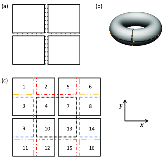
Figure 1: Schematic of configurations of the square lattice. (a) Configurations (i) and (ii) of the $L\times L$ lattice with open boundaries, in which inside edges are either disconnected [configuration (i)] or connected [configuration (ii)]. (b) Lattice configurations (iii) and (iv) with connected boundaries. The one with disconnected inner edges [configuration (iii)] is equivalent to the configuration (ii) up to a translation along both $x$ and $y$ directions by $L/2$ sites. (c) Configuration of the representative tensor for the compound quadrupled lattice. The joining regions of adjacent segments are indicated by indices $\{4,7,10,13\}$, $\{8,3,14,9\}$, $\{12,15,2,5\}$, and $\{16,11,6,1\}$, on which $U_{adj}$ should be imposed separately.

As a test case, the two-dimensional scheme is examined by a tight-binding model, a single particle hopping on a square lattice with a Hamiltonian

$$H=\sum_{x,y}[(ua_{x+1,y}^{\dagger}a_{x,y}+h.c.)+(va_{x,y+1}^{\dagger}a_{x,y}+h.c.)],$$ (3)

where $a_{x,y}^{\dagger}$ and $a_{x,y}$ are the creation and annihilation operators on the site $(x,y)$ and the hopping parameters are set as $u=-1$ and $v=-3/2$. The Hamiltonians of an $L=64$ square lattice with various boundary configurations are exactly diagonalized of which the eigenstates of configurations (ii) and (iv) are recorded as $|\psi_{j}\rangle$ and $|\psi_{j}^{p}\rangle$, respectively. Unitary $U_{adj}$’s can be built for the present system through full correspondences of the derived bases, which enables us to calculate states for the quadrupled lattice at any energy level. Starting from $m$ states $\{|\psi_{j}\rangle\}$ closest to a particular energy, the $4m$ basis states of the compound periodic lattice are generated and divided into four sets, $\{|\Psi_{j}^{\pm,\pm}\rangle,j=1,\cdots,m\}$, in which $``\pm"$ denotes the symmetric or anti-symmetric property of states under $\hat{t}_{x(y)}\equiv\hat{\mathcal{T}}_{x(y)}^{L}$, translations along the $x$ $(y)$ direction by $L$ sites. The lowest energies of the $L=128$ system achieved by the algorithm via $U_{adj}^{(1)}$ are shown in Table II, with which the exact energies and the energies achieved by the primitive NRG are presented for reference.

Table 2: Lowest energies of the $L=128$ square lattice with periodic boundary conditions achieved by the regularized NRG algorithm via the prescription $U_{adj}^{(1)}$. The energies are calculated in separated spaces of the four sets of basis states $\{|\Psi_{j}^{\pm,\pm}\rangle,j=1,\cdots,m\}$ with $m=64$ and are listed according to their values. The results recover the exact energies to $4$-$5$ digits and exhibit correct order, while the results obtained by the primitive NRG scheme are quite inaccurate and fail to yield the same ordering.

	$\{\hat{t}_{x},\hat{t}_{y}\}$	Exact	Regularized RG	Primitive RG		$\{\hat{t}_{x},\hat{t}_{y}\}$	Exact	Regularized RG	Primitive RG
$E_{0}$	$\{+,+\}$	-5.00000	-4.99960	-4.99462	$E_{8}$	$\{-,-\}$	-4.99398	-4.99386	-4.97853
$E_{1}$	$\{-,+\}$	-4.99759	-4.99732	-4.99431	$E_{9}$	$\{+,+\}$	-4.99037	-4.99011	-4.98698
$E_{2}$	$\{-,+\}$	-4.99759	-4.99728	-4.98821	$E_{10}$	$\{+,+\}$	-4.99037	-4.99009	-4.98314
$E_{3}$	$\{+,-\}$	-4.99639	-4.99623	-4.99417	$E_{11}$	$\{+,-\}$	-4.98676	-4.98674	-4.98494
$E_{4}$	$\{+,-\}$	-4.99639	-4.99617	-4.98653	$E_{12}$	$\{+,-\}$	-4.98676	-4.98672	-4.97730
$E_{5}$	$\{-,-\}$	-4.99398	-4.99395	-4.99387	$E_{13}$	$\{+,-\}$	-4.98676	-4.98668	-4.97698
$E_{6}$	$\{-,-\}$	-4.99398	-4.99391	-4.98776	$E_{14}$	$\{+,-\}$	-4.98676	-4.98666	-4.96774
$E_{7}$	$\{-,-\}$	-4.99398	-4.99389	-4.98463	$E_{15}$	$\{+,+\}$	-4.98555	-4.98541	-4.97742

Performance of the algorithm employing the prescription $U_{adj}^{(2)}$ on the above two models, the spin-$1$ Heisenberg chain and the tight-binding model, displays that it is slightly less accurate than that utilizing $U_{adj}^{(1)}$. For example, the algorithm using $U_{adj}^{(2)}$ yields a ground-state energy $E_{0}\approx-22.43222$ for the 16-site Heisenberg chain provided that the same amount of $47$ states are kept. Nevertheless, it is of interest to mention an exceptional case of the tight-binding model, where the numerical calculation discloses that the symmetric basis states $\{|\Psi_{j}^{+,+}\rangle\}$, generated via imposing $U_{adj}^{(2)}$’s on the state vectors of direct sum $|\psi_{j}\rangle\oplus|\psi_{j}\rangle\oplus|\psi_{j}\rangle\oplus|\psi_{j}\rangle$, are exact eigenstates of the quadrupled system with periodic boundary conditions. In view that the intercepted state vector of any joining segments with fourfold adjacent edges represents a basis state of the lattice configuration $(iii)$, the transformation $U_{adj}^{(2)}$ on each of those joining segments maps it precisely onto $|\psi_{j}^{p}\rangle$, a basis state of the lattice configuration (iv). That is to say, direct combinations of basis states of the periodic $L\times L$ block, $|\psi_{j}^{p}\rangle\oplus|\psi_{j}^{p}\rangle\oplus|\psi_{j}^{p}\rangle\oplus|\psi_{j}^{p}\rangle$, already give rise to one fourth of the full set of exact solutions of the compound $2L\times 2L$ system. This result is indeed general: it is independent of the size $L$ and applies also to the one-dimensional tight-binding model wherein it is very easy to verify.

In the present algorithm at least two truncated basis sets are kept and they should be expressed in a complete set of spin bases. This should be the case at each iteration since any such truncated set is too incomplete to represent other basis states with different boundary configurations. As a result, repetition of the described RG procedure is constrained by the capacity of storing vectors with exponentially growing dimensions. In this sense, the regularized NRG scheme is applicable to finite lattices rather than the infinite one since the iterative performance of the procedure for the latter system will break down inevitably. This indeed offers the underlying cause which supports partly the folklore stating that all real-space RG schemes are necessarily inaccurate for lattice systems.

Alternatively, if one chooses to sacrifice some of the accuracy, an iterative procedure could be achieved, at least for one-dimensional systems, by projecting the derived basis states, e.g., those of $H_{2L}$ and $H_{2L}^{p}$, on the tensor product space of the $m$ states kept to get bases $|\tilde{\psi}_{j}\rangle$ and $|\tilde{\psi}_{j}^{p}\rangle$ of dimension $m^{2}$. The prescribed transformation, $\tilde{U}_{adj}$, could be built by virtue of these basis states which is then imposed on the states $|\tilde{\psi}_{j}\rangle\otimes|\tilde{\psi}_{j^{\prime}}\rangle$ to generate basis states for the pair of Hamiltonians with larger size. The truncation of the algorithm here is distinctly different from that of the primitive NRG scheme in view that the $m$ states kept are taken from a Hilbert space of dimension $m^{4}$ instead of dimension $m^{2}$. It is also worthy to note that the strategy adopted here, projecting the basis states of the compound block onto a restricted space of tensor product states of subsystems, is what has been done in the contractor RG method core1 ; core2 ; core3 . In comparison, the interblock coupling of the effective Hamiltonian in the latter scheme is obtained by substracting the contributions of contained subclusters, while in the present scheme the effective Hamiltonian of the compound system could be constructed directly by virtue of the regularized basis states.

The author thanks H.-G. Luo for helpful discussions. Support of the National Natural Science Foundation of China (Grant No. 10874254) is acknowledged.

References

- (1) K.G. Wilson, Rev. Mod. Phys. 47, 773 (1975).
- (2) J.N. Fields, Phys. Rev. B 19, 2637 (1979).
- (3) J.N. Fields, H.W. J. Blote, and J.C. Bonner, J. Appl. Phys. 50, 1807 (1979).
- (4) J.W. Bray and S.T. Chui, Phys. Rev. B 19, 4876 (1979).
- (5) P.A. Lee, Phys. Rev. Lett. 42, 1492 (1979).
- (6) P.A. Lee and D.S. Fisher, Phys. Rev. Lett. 47, 882 (1981).
- (7) S.R. White and R.M. Noack, Phys. Rev. Lett. 68, 3487 (1992).
- (8) S.R. White, Phys. Rev. Lett. 69, 2863 (1992).
- (9) S.R. White, Phys. Rev. B 48, 10345 (1993).
- (10) S.R. White, Phys. Rep. 301, 187 (1998).
- (11) M.A. Nielsen and I.L. Chuang, Quantum Computation and Quantum Information (Cambridge University Press 2000).
- (12) X. Chen, Z.-C. Gu, X.-G. Wen, Phys. Rev. B 82, 155138 (2010).
- (13) X. Chen, Z.-C. Gu, Z.-X. Liu, and X.-G. Wen, Phys. Rev. B 87, 155114 (2013).
- (14) R.M. Noack and S.R. White, Phys. Rev. B 47, 9243 (1993).
- (15) For topologically nontrivial systems the choice of the phases might not be irrelevant and it should be investigated elsewhere.
- (16) A. Moreo, Phys. Rev. B 35, 8562 (1987).
- (17) H.Q. Lin, Phys. Rev. B 42, 6561 (1990).
- (18) A. Bohm and M. Loewe, Quantum Mechanics: Foundations and Applications (New York: Springer-Verlag, 3rd ed., 1993).
- (19) J.-Q. Chen, M.-J. Gao, and G.-Q. Ma, Phys. Rev. Mod. 57, 211 (1985).
- (20) C.J. Morningstar and M. Weinstein, Phys. Rev. Lett. 73, 1873 (1994).
- (21) M. Weinstein, Phys. Rev. B 63, 174421 (2001).
- (22) J.-P. Malrieu and N. Guihéry, Phys. Rev. B 63, 085110 (2001).