Ring-polymer instanton theory of electron transfer in the nonadiabatic limit

Abstract

We take the golden-rule instanton method derived in the previous paper [arXiv:1509.04919] and reformulate it using a ring-polymer approach. This gives equations which can be used to compute the rates of electron-transfer reactions in the nonadiabatic (golden-rule) limit numerically within a semiclassical approximation. The multidimensional ring-polymer instanton trajectories are obtained efficiently by minimization of the action. In this form, comparison with Wolynes’ quantum instanton method [P. G. Wolynes, J. Chem. Phys. 87, 6559 (1987)] is possible and we show that our semiclassical approach is the steepest-descent limit of this method. We discuss advantages and disadvantages of both methods and give examples of where the new approach is more accurate.

I Introduction

In the previous paper, henceforth referred to as Paper I, Richardson, Bauer, and Thoss we outlined a derivation of a golden-rule instanton theory for computing electron-transfer rates in the nonadiabatic limit. This was based on a time-independent methodology using Fermi’s golden rule, which is correct in the limit that the electronic coupling is weak. In these equations, we substituted the semiclassical limit of the Green’s functions describing nuclear dynamics on one of two potential-energy surfaces at a given energy. A number of steepest-descent integrations led to a formula which defines the rate in terms of the action of an imaginary-time periodic orbit, known as the instanton.

In this paper, we show how this approximate formulation of the rate can be evaluated numerically to treat electron transfer in large complex systems. We describe how the golden-rule instanton trajectory can be discretized, allowing it to be located efficiently using multidimensional optimization techniques. This is done using a ring-polymer instanton approach similar to that used by related methods employing a single Born-Oppenheimer surface, including the adiabatic rate Richardson and Althorpe (2009); Andersson et al. (2009); Andersson, Goumans, and Arnaldsson (2011); Goumans and Kästner (2010); *Goumans2011Hmethanol; *Meisner2011isotope; *Rommel2012enzyme; Rommel, Goumans, and Kästner (2011); Rommel and Kästner (2011); Althorpe (2011); Pérez de Tudela et al. (2014) as well as tunnelling splitting calculations. Richardson and Althorpe (2011); Richardson, Althorpe, and Wales (2011); Richardson et al. (2013); Kawatsu and Miura (2014); *Kawatsu2015NH3

In contrast, early applications of instanton approaches employed a method known as “shooting” to locate the required instanton trajectory. This method ran classical dynamics on the inverted potential-energy surface and attempted to choose the correct initial conditions such that the trajectory closed into a periodic orbit. Chapman, Garrett, and Miller (1975) Because the trajectories are unstable, this approach is inefficient and in general limited to treating systems of very few dimensions. Benderskii, Makarov, and Wight (1994)

Many alternative methods exist for computing nonadiabatic rate constants based on a time-dependent formulation. These include exact wave function calculations Wang, Thoss, and Miller (2001); *Thoss2001hybrid; Wang, Skinner, and Thoss (2006) and real-time path-integral calculations for system-bath models. Marchi and Chandler (1991); Topaler and Makri (1996); Mühlbacher and Egger (2003); *Muehlbacher2004asymmetric; Ananth and Miller III (2012) For more general systems approximate trajectory-based methods have been developed Huo, Miller III, and Coker (2013); *Huo2015PLDM; Kapral (2015); Sun, Wang, and Miller (1998); *Wang1999mapping; Cotton, Igumenshchev, and Miller (2014); Schwerdtfeger, Soudackov, and Hammes-Schiffer (2014); Landry and Subotnik (2012) including extensions of ring-polymer molecular dynamics. Richardson and Thoss (2013); Ananth (2013); Menzeleev, Ananth, and Miller (2011); *Kretchmer2013ET; *Menzeleev2014kinetic; Shushkov, Li, and Tully (2012)

There are some difficulties with time-dependent methods however, as the flux correlation functions Miller, Schwartz, and Tromp (1983) can become very oscillatory when describing electron transfer. Huo, Miller III, and Coker (2013) Some work towards avoiding these problems has been achieved by modifying the correlation function formalism to remove the oscillations, although without affecting the long-time limit which defines the exact rate. Richardson and Thoss (2014) This simplification was achieved in part by considering a time-independent picture, as we have also done in the derivation of the golden-rule instanton.

Although the derivation is very different, we also show how our result can be related to Wolynes’ quantum instanton method. Wolynes (1987) This approach uses an approximation based on the short-time behaviour of the flux correlation function in the nonadiabatic (golden-rule) limit and is evaluated using path-integral Monte Carlo. The method has been applied to study electron transfers in chemically and biologically relevant systems. Bader, Kuharski, and Chandler (1990); Zheng, McCammon, and Wolynes (1989); *Zheng1991ET Our new derivation of a golden-rule rate offers more insight into the approximations made by such methods and is in some cases more accurate.

An outline of the paper is as follows. The main results from Paper I are summarized in Sec. II, and we show how the action integral is discretized and its derivatives obtained in Sec. III. We thus obtain a ring-polymer instanton formulation for the electron-transfer rate, which is related to Wolynes’ quantum instanton approach in Sec. IV. Suggestions for how the instanton approach could be applied numerically to complex systems are presented in Sec. V, which introduces an efficient algorithm for locating the instanton trajectories. This is applied to an example system in Sec. VI to analyse its convergence properties, and Sec. VII concludes the article.

II Summary of the Golden-Rule Instanton Approach

It was shown in Paper I that the instanton relevant to the electron-transfer problem is an imaginary-time periodic orbit. This is formed of two trajectories which travel on the upside-down reactant, $V_{0}(\mathsf{x})$, or product, $V_{1}(\mathsf{x})$, $f$-dimensional potential-energy surfaces. They each bounce once and join smoothly together at a point, $\mathsf{x}^{\ddagger}$, found on the crossing seam, defined by $V_{0}(\mathsf{x})=V_{1}(\mathsf{x})$.

In this paper, we deal only with imaginary-time trajectories and thus depart from the notation of Paper I by dropping the bar over imaginary properties. The Euclidean action along one trajectory, either on the reactant $(n=0)$ or product $(n=1)$ surface, is Feynman and Hibbs (1965); Miller (1971)

$$S_{n}\equiv S_{n}(\mathsf{x}^{\prime},\mathsf{x}^{\prime\prime},\tau_{n}) =\int_{0}^{\tau_{n}}\left[{\tfrac{1}{2}}m\left|\frac{\partial{\mathsf{x}(\tau)}}{\partial{\tau}}\right|^{2}+V_{n}\big{(}\mathsf{x}(\tau)\big{)}\right]\mathrm{d}\tau,$$ (1)

where the trajectory, $\mathsf{x}(\tau)$, travels through the classically forbidden region from $\mathsf{x}(0)=\mathsf{x}^{\prime}$ to $\mathsf{x}(\tau_{n})=\mathsf{x}^{\prime\prime}$, or equivalently in the opposite direction. A complete periodic orbit which runs in imaginary time $\beta\hbar$ has the action

$${S}(\mathsf{x}^{\prime},\mathsf{x}^{\prime\prime},\tau)={S}_{0}(\mathsf{x}^{\prime},\mathsf{x}^{\prime\prime},\beta\hbar-\tau)+{S}_{1}(\mathsf{x}^{\prime\prime},\mathsf{x}^{\prime},\tau),$$ (2)

where $\tau\in[0,\beta\hbar]$. The particular periodic orbit required is that which is stationary in $\mathsf{x}^{\prime}$, $\mathsf{x}^{\prime\prime}$ and $\tau$. In the following all terms are evaluated at this stationary point, at which $\mathsf{x}^{\prime}=\mathsf{x}^{\prime\prime}=\mathsf{x}^{\ddagger}$.

The golden-rule instanton method derived in Paper I gives a semiclassical approximation to the rate in terms of the actions along these trajectories. Two equivalent formulae are

$$k_{\text{SC}}Z_{0} =\sqrt{2\pi\hbar}\,\frac{\Delta^{2}}{\hbar^{2}}\sqrt{\frac{{C}_{0}{C}_{1}}{-\Sigma}}\,\mathrm{e}^{-{S}/\hbar}$$ (3)

$$=\sqrt{2\pi\hbar}\,\frac{\Delta^{2}}{\hbar^{2}}\sqrt{\frac{{C}_{0}{C}_{1}}{{C}}}\left(-\frac{\mathrm{d}^{2}{S}}{\mathrm{d}\tau^{2}}\right)^{-{\tfrac{1}{2}}}\,\mathrm{e}^{-{S}/\hbar},$$ (4)

where the van-Vleck prefactor for a trajectory is given by

$${C}_{n} =\left|-\frac{\partial^{2}{S}_{n}}{\partial\mathsf{x}^{\prime}\partial\mathsf{x}^{\prime\prime}}\right|$$ (5)

and the other prefactors are

$${C} =\left|\begin{matrix}\frac{\partial^{2}{S}}{\partial\mathsf{x}^{\prime}\partial\mathsf{x}^{\prime}}&\frac{\partial^{2}{S}}{\partial\mathsf{x}^{\prime}\partial\mathsf{x}^{\prime\prime}}\\ \frac{\partial^{2}{S}}{\partial\mathsf{x}^{\prime\prime}\partial\mathsf{x}^{\prime}}&\frac{\partial^{2}{S}}{\partial\mathsf{x}^{\prime\prime}\partial\mathsf{x}^{\prime\prime}}\end{matrix}\right|$$ (6)

$$\Sigma =\left|\begin{matrix}\frac{\partial^{2}{S}}{\partial\mathsf{x}^{\prime}\partial\mathsf{x}^{\prime}}&\frac{\partial^{2}{S}}{\partial\mathsf{x}^{\prime}\partial\mathsf{x}^{\prime\prime}}&\frac{\partial^{2}{S}}{\partial\mathsf{x}^{\prime}\partial\tau}\\ \frac{\partial^{2}{S}}{\partial\mathsf{x}^{\prime\prime}\partial\mathsf{x}^{\prime}}&\frac{\partial^{2}{S}}{\partial\mathsf{x}^{\prime\prime}\partial\mathsf{x}^{\prime\prime}}&\frac{\partial^{2}{S}}{\partial\mathsf{x}^{\prime\prime}\partial\tau}\\ \frac{\partial^{2}{S}}{\partial\tau\partial\mathsf{x}^{\prime}}&\frac{\partial^{2}{S}}{\partial\tau\partial\mathsf{x}^{\prime\prime}}&\frac{\partial^{2}{S}}{\partial\tau^{2}}\\ \end{matrix}\right|.$$ (7)

These formulae for the golden-rule instanton method were used in Paper I to obtain the rate of electron transfer in a few special systems for which the bounce trajectories and corresponding action is known analytically. In order to apply the method to more general problems with anharmonic potentials, we will require numerical methods which are able to locate the instanton trajectory and evaluate the action and its derivatives. This is the topic addressed in this paper.

III Discretization Scheme

In this section, we show how the action integral, Eq. (1), can be defined from a discretized form of an imaginary-time trajectory. This is based on the ring-polymer instanton method, Richardson and Althorpe (2009) which has been successfully used in adiabatic, single-surface, rate calculations Andersson et al. (2009); Rommel, Goumans, and Kästner (2011) as well as the evaluation of tunnelling splittings. Richardson and Althorpe (2011); Richardson, Althorpe, and Wales (2011); Richardson et al. (2013) It relies on the fact that a classical trajectory is known to give a stationary value of the action, with respect to any deviation along its length except at the end points. Whittaker (1988); Goldstein, Poole, and Safko (2002)

We also describe how second derivatives of the action can be evaluated directly without resorting to taking finite differences between instantons optimized under various conditions. The approach we use for this follows closely the method of implicit differentiation described in LABEL:Althorpe2011ImF, which we extend to obtain all the derivatives required for the golden-rule instanton method.

According to our golden-rule approach, Richardson, Bauer, and Thoss we only need to study the dynamics on one of the two potential-energy surfaces at any time. This section would thus also be directly applicable to single-surface reactions, simply by dropping the subscript $n$.

We consider an imaginary-time pathway of length $\tau_{n}$ between the points $\mathsf{x}^{\prime}\equiv\mathsf{x}_{0}$ and $\mathsf{x}^{\prime\prime}\equiv\mathsf{x}_{N_{n}}$, which passes through the intermediate points $\{\mathsf{x}_{1},\dots,\mathsf{x}_{N_{n}-1}\}$ at a set of discrete times. The imaginary-time intervals between each point are $\delta\tau_{i}=\epsilon_{i}\tau_{n}$, with $i\in\{1,\dots,N_{n}\}$ such that each $\epsilon_{i}\in[0,1]$ and $\sum_{i=1}^{N_{n}}\epsilon_{i}=1$. The velocity along a given pathway at these times is given by $|\mathsf{x}_{i}-\mathsf{x}_{i-1}|/\epsilon_{i}\tau_{n}$ and the action by

$$S_{n}(\mathsf{x}_{0},\dots,\mathsf{x}_{N_{n}};\tau_{n})=\sum_{i=1}^{N_{n}}\frac{m|\mathsf{x}_{i}-\mathsf{x}_{i-1}|^{2}}{2\epsilon_{i}\tau_{n}}\\ +\sum_{i=1}^{N_{n}}\epsilon_{i}\tau_{n}\frac{V_{n}(\mathsf{x}_{i-1})+V_{n}(\mathsf{x}_{i})}{2},$$ (8)

where the first term originates from a trapezium-rule integration of the kinetic energy along the pathway, and the second of the potential energy. This is the general form allowing for uneven imaginary time intervals Rommel and Kästner (2011) and would simplify to the usual case with $\epsilon_{i}=1/{N_{n}}$. Note that here an open-ended pathway is described such that no cyclic indices are implied.

The points $\tilde{\mathsf{x}}_{i}$ for $i\in\{1,\dots,N_{n}-1\}$, which give the coordinates along the classical trajectory, are those which give a stationary value of $S_{n}$, i.e. those which solve

$$\frac{\tilde{\mathsf{x}}_{i}-\tilde{\mathsf{x}}_{i-1}}{\epsilon_{i}}+\frac{\tilde{\mathsf{x}}_{i}-\tilde{\mathsf{x}}_{i+1}}{\epsilon_{i+1}}+\frac{(\epsilon_{i}+\epsilon_{i+1})\tau_{n}^{2}}{2m}\frac{\partial{V_{n}}}{\partial{\tilde{\mathsf{x}}_{i}}}=\mathsf{0}.$$ (9)

The action along the trajectory is therefore $S_{n}(\mathsf{x}^{\prime},\mathsf{x}^{\prime\prime},\tau_{n})\equiv\lim_{N_{n}\rightarrow\infty}\tilde{S}_{n}(\mathsf{x}^{\prime},\mathsf{x}^{\prime\prime},\tau_{n})$, where $\tilde{S}_{n}(\mathsf{x}^{\prime},\mathsf{x}^{\prime\prime},\tau_{n})=S_{n}(\tilde{\mathsf{x}}_{0},\tilde{\mathsf{x}}_{1},\dots,\tilde{\mathsf{x}}_{N_{n}};\tau_{n})$ and $\tilde{\mathsf{x}}_{0}\equiv\mathsf{x}^{\prime}$, $\tilde{\mathsf{x}}_{N_{n}}\equiv\mathsf{x}^{\prime\prime}$.

In fact the dominant classical trajectory between two end points in a given imaginary time will be the global minimum of Eq. (8) with respect to the intermediate points. This can be obtained by employing a multidimensional optimization routine such as the limited memory Broyden-Fletcher-Goldfarb-Shanno (l-BFGS) algorithm Zhu et al. (1997) in the same way as is done for tunnelling splitting calculations. Richardson and Althorpe (2011); Richardson, Althorpe, and Wales (2011) However, the end points, $\mathsf{x}^{\ddagger}$, required for the instanton method are not in general known a priori, so the instanton trajectories cannot be obtained in this way. We discuss optimization methods which do not require knowledge of the end points in Sec. IV.

Differentiating Eq. (9) by the end points, $\mathsf{x}^{\prime}$ or $\mathsf{x}^{\prime\prime}$, gives equations which can be written in the following form:

$$\sum_{i^{\prime}=1}^{N_{n}-1}\sum_{j^{\prime}=1}^{f}J_{ij,i^{\prime}j^{\prime}}\frac{\partial{\tilde{x}_{i^{\prime}j^{\prime}}}}{\partial{x^{\prime}_{k}}} =\frac{\delta_{i1}\delta_{jk}}{N_{n}\epsilon_{1}}$$ (10a)

$$\sum_{i^{\prime}=1}^{{N_{n}}-1}\sum_{j^{\prime}=1}^{f}J_{ij,i^{\prime}j^{\prime}}\frac{\partial{\tilde{x}_{i^{\prime}j^{\prime}}}}{\partial{x^{\prime\prime}_{k}}} =\frac{\delta_{i\,{N_{n}}-1}\delta_{jk}}{N_{n}\epsilon_{N_{n}}},$$ (10b)

where the elements of the doubly indexed matrix $\mathbf{J}$ are defined by

$$J_{ij,i^{\prime}j^{\prime}}=\frac{\delta_{ii^{\prime}}-\delta_{i+1\,i^{\prime}}}{N_{n}\epsilon_{i}}\delta_{jj^{\prime}}+\frac{\delta_{ii^{\prime}}-\delta_{i-1\,i^{\prime}}}{N_{n}\epsilon_{i+1}}\delta_{jj^{\prime}}\\ +\delta_{ii^{\prime}}\frac{(\epsilon_{i}+\epsilon_{i+1})\tau_{n}^{2}}{2N_{n}m}\nabla^{2}_{jj^{\prime}}V_{n}(\tilde{\mathsf{x}}_{i}).$$ (11)

Again the indices are not cyclic, i.e. the matrix is banded with bandwidth $f$. This definition is equivalent to that given in LABEL:Althorpe2011ImF when the time-steps are equal. Equations (10) can be solved numerically for the derivatives of $\tilde{\mathsf{x}}$ using standard linear-algebra routines. Note that these partial derivatives imply that $\tau_{n}$ and one end point are kept fixed while the rest of the pathway is allowed to re-optimize itself as the other end point varies.

Other terms are found by differentiating Eq. (9) by $\tau_{n}$ to give

$$\sum_{i^{\prime}=1}^{N_{n}-1}\sum_{j^{\prime}=1}^{f}J_{ij,i^{\prime}j^{\prime}}\frac{\partial{\tilde{x}_{i^{\prime}j^{\prime}}}}{\partial{\tau_{n}}} =-\frac{(\epsilon_{i}+\epsilon_{i+1})\tau_{n}}{N_{n}m}\frac{\partial{V_{n}}}{\partial{\tilde{x}_{ij}}},$$ (12)

which we solve for $\frac{\partial{\tilde{\mathsf{x}}_{i}}}{\partial{\tau_{n}}}$.

Using the fact that $\tilde{S}_{n}$ is stationary with respect to differentiation by $\tilde{\mathsf{x}}_{i}$ gives

$$\frac{\partial\tilde{S}_{n}}{\partial\mathsf{x}^{\prime}} =\frac{m(\mathsf{x}^{\prime}-\tilde{\mathsf{x}}_{1})}{\epsilon_{1}\tau_{n}}+\frac{\epsilon_{1}\tau_{n}}{2}\mathbf{\nabla}V_{n}(\mathsf{x}^{\prime})$$ (13a)

$$\frac{\partial\tilde{S}_{n}}{\partial\mathsf{x}^{\prime\prime}} =\frac{m(\mathsf{x}^{\prime\prime}-\tilde{\mathsf{x}}_{N_{n}-1})}{\epsilon_{N_{n}}\tau_{n}}+\frac{\epsilon_{N_{n}}\tau_{n}}{2}\mathbf{\nabla}V_{n}(\mathsf{x}^{\prime\prime})$$ (13b)

$$\frac{\partial\tilde{S}_{n}}{\partial\tau_{n}} =-\sum_{i=1}^{N_{n}}\frac{m|\tilde{\mathsf{x}}_{i}-\tilde{\mathsf{x}}_{i-1}|^{2}}{2\epsilon_{i}\tau_{n}^{2}}+\sum_{i=1}^{N_{n}}\epsilon_{i}\frac{V_{n}(\tilde{\mathsf{x}}_{i-1})+V_{n}(\tilde{\mathsf{x}}_{i})}{2}.$$ (13c)

Differentiating again, we obtain the second derivatives:

$$\frac{\partial^{2}\tilde{S}_{n}}{\partial x_{j}^{\prime}\partial x_{k}^{\prime}} =\frac{m}{\epsilon_{1}\tau_{n}}\left(\delta_{jk}-\frac{\partial{\tilde{x}_{1j}}}{\partial{x^{\prime}_{k}}}\right)+\frac{\epsilon_{1}\tau_{n}}{2}\nabla^{2}_{jk}V_{n}(\mathsf{x}^{\prime})$$ (14a)

$$\frac{\partial^{2}\tilde{S}_{n}}{\partial x_{j}^{\prime}\partial x_{k}^{\prime\prime}} =-\frac{m}{\epsilon_{1}\tau_{n}}\frac{\partial{\tilde{x}_{1j}}}{\partial{x^{\prime\prime}_{k}}}$$ (14b)

$$\frac{\partial^{2}\tilde{S}_{n}}{\partial x_{j}^{\prime\prime}\partial x_{k}^{\prime\prime}} =\frac{m}{\epsilon_{N_{n}}\tau_{n}}\left(\delta_{jk}-\frac{\partial{\tilde{x}_{{N_{n}}-1\,j}}}{\partial{x^{\prime\prime}_{k}}}\right)+\frac{\epsilon_{N_{n}}\tau_{n}}{2}\nabla^{2}_{jk}V_{n}(\mathsf{x}^{\prime\prime})$$ (14c)

$$\frac{\partial^{2}\tilde{S}_{n}}{\partial\mathsf{x}^{\prime}\partial\tau_{n}} =-\frac{m(\mathsf{x}^{\prime}-\tilde{\mathsf{x}}_{1})}{\epsilon_{1}\tau_{n}^{2}}-\frac{m}{\epsilon_{1}\tau_{n}}\frac{\partial{\tilde{\mathsf{x}}_{1}}}{\partial{\tau_{n}}}+\frac{\epsilon_{1}}{2}\frac{\partial{V_{n}}}{\partial{\mathsf{x}^{\prime}}}$$ (14d)

$$\frac{\partial^{2}\tilde{S}_{n}}{\partial\mathsf{x}^{\prime\prime}\partial\tau_{n}} =-\frac{m(\mathsf{x}^{\prime\prime}-\tilde{\mathsf{x}}_{{N_{n}}-1})}{\epsilon_{N_{n}}\tau_{n}^{2}}-\frac{m}{\epsilon_{N_{n}}\tau_{n}}\frac{\partial{\tilde{\mathsf{x}}_{{N_{n}}-1}}}{\partial{\tau_{n}}}+\frac{\epsilon_{N_{n}}}{2}\frac{\partial{V_{n}}}{\partial{\mathsf{x}^{\prime\prime}}}$$ (14e)

$$\frac{\partial^{2}\tilde{S}_{n}}{\partial\tau_{n}^{2}} =\sum_{i=1}^{N_{n}}\frac{m|\tilde{\mathsf{x}}_{i}-\tilde{\mathsf{x}}_{i-1}|^{2}}{\epsilon_{i}\tau_{n}^{3}}+\sum_{i=1}^{{N_{n}}-1}\frac{\epsilon_{i}+\epsilon_{i+1}}{2}\frac{\partial{V_{n}}}{\partial{\tilde{\mathsf{x}}_{i}}}\cdot\frac{\partial{\tilde{\mathsf{x}}_{i}}}{\partial{\tau_{n}}}$$

$$\quad-\sum_{i=1}^{{N_{n}}-1}\frac{m}{\tau_{n}^{2}}\left(\frac{\tilde{\mathsf{x}}_{i}-\tilde{\mathsf{x}}_{i-1}}{\epsilon_{i}}+\frac{\tilde{\mathsf{x}}_{i}-\tilde{\mathsf{x}}_{i+1}}{\epsilon_{i+1}}\right)\cdot\frac{\partial{\tilde{\mathsf{x}}_{i}}}{\partial{\tau_{n}}}.$$ (14f)

Partial derivatives of $S_{n}$ are approximated by these formulae, which become exact in the ${N_{n}}\rightarrow\infty$ limit. Assuming that the instanton trajectories have already been found, these derivatives can be applied in the prefactor of Eq. (3), using Eq. (7) and Eq. (2), to give the golden-rule instanton rate.

In contrast to standard approaches where the eigenvalues of a $Nf\times Nf$ matrix are required for the prefactor, the most difficult task in this approach is the solution of the linear equations, Eqs. (10) and (12). Because $\mathbf{J}$ is the Hessian matrix about the minimum pathway, it is positive definite, and the equations can be solved efficiently using a Cholesky decomposition, taking advantage of the banded nature of the matrix. Press et al. (1992)

This approach is not limited to the current application but may also significantly improve the efficiency of other instanton methods, for which the diagonalization can be a considerably time-consuming task for high-dimensional systems. We shall discuss the use of such an approach to improve the efficiency of adiabatic rate calculations in a forthcoming paper.

IV Ring-polymer instanton formulation

So far, we have only dealt with open-ended trajectories, whose end points are as yet unknown. In this section, we extend this methodology to obtain the pathway for the total periodic orbit. This orbit is simply the combination of a trajectory on the reactant surface with another on the product surface and has total imaginary time $\beta\hbar$.

We divide up the total orbit into $N$ segments, with the first $N_{0}$ on $\ket{0}$ and the remaining $N_{1}=N-N_{0}$ on $\ket{1}$ as in Fig. 1. Equal time-step intervals, $\epsilon_{i}=1/N_{n}$, will be assumed here but other choices may slightly improve efficiency. Rommel and Kästner (2011)

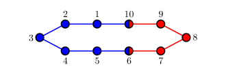
Figure 1: Schematic showing the ring-polymer beads which discretize the instanton for the case of $N_{0}=6$ and $N_{1}=4$. Those on the left coloured in blue have the electronic configuration of the reactant state $\ket{0}$ and those on the right in red of the product $\ket{1}$. Beads $N_{0}$ and $N$ are located at the hopping point $\mathsf{x}^{\ddagger}$ and contribute to the action of both trajectories.

There is a special case that the time intervals on both trajectories are equal, all with length $\beta_{N}\hbar$, where $\beta_{N}=\beta/N$. This can only be obtained in practice if the imaginary times along each trajectory, $\tau_{n}=N_{n}\beta_{N}\hbar$, are known a priori. Such cases arise for example if the reaction is symmetric, where the stationary value is known to be $\tau=\beta\hbar/2$, or if the instanton has already been obtained by an alternative method, such as those introduced in Sec. V.

In this case, we have a formulation similar to path-integral Parrinello and Rahman (1984) and ring-polymer molecular dynamics, Richardson and Althorpe (2009); Habershon et al. (2013) which were obtained from a discretization of the quantum Boltzmann operator. The resulting set of $N$ coordinates are called beads and, via a quantum-classical correspondence, Chandler and Wolynes (1981) are equivalent to a ring polymer of classical particles connected together by harmonic springs.

It is a good idea to use the $N$-bead steepest-descent approximation to the reactant partition function, Kleinert (2006)

$$Z_{0} =\prod_{j=1}^{f}\left[2\sinh\frac{\beta\hbar\tilde{\omega}_{j}}{2}\right]^{-1}$$ (15)

$$\tilde{\omega}_{j} =\frac{2}{\beta_{N}\hbar}\sinh^{-1}\frac{\beta_{N}\hbar\omega_{j}}{2},$$ (16)

as this is known to benefit from a cancellation of errors with the $N$-bead instanton calculation and improve convergence of the rate. Andersson et al. (2009) Here $\omega_{j}$ are the normal-mode frequencies at the minimum of $V_{0}(\mathsf{x})$; if there are translation or rotational modes, the formula should be modified appropriately.

The total action along the two joined pathways is given by

$$\beta_{N}U_{N}(\mathbf{x})=S_{0}(\mathsf{x}_{N},\mathsf{x}_{1},\dots,\mathsf{x}_{N_{0}};N_{0}\beta_{N}\hbar)\\ +S_{1}(\mathsf{x}_{N_{0}},\dots,\mathsf{x}_{N};N_{1}\beta_{N}\hbar),$$ (17)

such that the $N$-bead ring-polymer potential is

$$U_{N}(\mathbf{x})=\sum_{i=1}^{N}\frac{m}{2\beta_{N}^{2}\hbar^{2}}|\mathsf{x}_{i+1}-\mathsf{x}_{i}|^{2}\\ +{\tfrac{1}{2}}V_{0}(\mathsf{x}_{N})+\sum_{i=1}^{N_{0}-1}V_{0}(\mathsf{x}_{i})+{\tfrac{1}{2}}V_{0}(\mathsf{x}_{N_{0}})\\ +{\tfrac{1}{2}}V_{1}(\mathsf{x}_{N_{0}})+\sum_{i=N_{0}+1}^{N-1}V_{1}(\mathsf{x}_{i})+{\tfrac{1}{2}}V_{1}(\mathsf{x}_{N}).$$ (18)

The positions of each bead are given by $\mathbf{x}=\{\mathsf{x}_{1},\dots,\mathsf{x}_{N}\}$, and cyclic indices are implied such that $\mathsf{x}_{0}\equiv\mathsf{x}_{N}$. This function can be minimized with respect to the positions of all beads to obtain the coordinates $\tilde{\mathbf{x}}=\{\tilde{\mathsf{x}}_{1},\dots,\tilde{\mathsf{x}}_{N}\}$ along both trajectories simultaneously. The hopping point is then identified as $\mathsf{x}^{\ddagger}=\tilde{\mathsf{x}}_{N_{0}}=\tilde{\mathsf{x}}_{N}$ and the action as $\tilde{S}=\beta_{N}\tilde{U}_{N}$, where $\tilde{U}_{N}=U_{N}(\tilde{\mathbf{x}})$. However, $\tau$, or equivalently the ratio $N_{0}/N_{1}$, is yet to be specified. It will therefore be necessary to compute the instanton for numerous values of $\tau$ to find the stationary point of $\tilde{U}_{N}$ with respect to $\tau$.

We now introduce the quantum instanton approach of Wolynes. Wolynes (1987) This method was derived using a steepest-descent evaluation of the time integral over the exact flux-flux correlation function within the golden-rule approximation and gives

$$k_{\text{QI}}Z_{0} =\sqrt{2\pi\hbar}\,\frac{\Delta^{2}}{\hbar^{2}}\left(-\frac{\mathrm{d}^{2}{\phi}}{\mathrm{d}{\tau}^{2}}\right)^{-{\tfrac{1}{2}}}\mathrm{e}^{-\phi(\tau)/\hbar}$$ (19)

$$\mathrm{e}^{-\phi(\tau)/\hbar} =\Lambda^{-Nf}\int\mathrm{e}^{-\beta_{N}U_{N}(\mathbf{x})}\,\mathrm{d}\mathbf{x},$$ (20)

where the prefactor is $\Lambda=\sqrt{2\pi\beta_{N}\hbar^{2}/m}$. It is here assumed for simplicity, that the electronic coupling, $\Delta$, is approximately constant, although the formulation could be generalized without affecting our findings. In practice the integrals are computed using a discrete path-integral Monte Carlo simulation, and $\tau=N_{1}\beta_{N}\hbar$ is chosen in the range $[0,\beta\hbar]$ such that $\frac{\mathrm{d}{\phi}}{\mathrm{d}{\tau}}=0$. Taking the second derivative of Eq. (20) gives Cao and Voth (1997); *Cao1998erratum

$$-\frac{1}{\hbar}\frac{\mathrm{d}^{2}{\phi}}{\mathrm{d}{\tau}^{2}}\,\mathrm{e}^{-\phi(\tau)/\hbar} =\frac{\Lambda^{-Nf}}{\hbar^{2}}\int V_{-}(\mathsf{x}^{\prime})V_{-}(\mathsf{x}^{\prime\prime})\,\mathrm{e}^{-\beta_{N}U_{N}(\mathbf{x})}\,\mathrm{d}\mathbf{x},$$ (21)

where $V_{-}(\mathsf{x})=V_{0}(\mathsf{x})-V_{1}(\mathsf{x})$. The second derivative of $\phi$ is negative and thus corresponds to a stationary point which is a maximum along $\tau$.

The derivation is similar in spirit to that used to obtain the quantum instanton approach for Born-Oppenheimer systems described in LABEL:Vanicek2005QI, as it also employs a steepest-descent integration along the real-time coordinate of a flux-flux correlation function. The single-surface quantum instanton approach is however not a semiclassical approximation in the sense that it gives the correct leading order of $\hbar$. This is most easily seen from the fact that it does not reproduce correct results for a free-particle or in the classical limit. Miller et al. (2003) Wolynes’ formula, Eq. (19), is also not exact in the high-temperature limit in general. However, it is known that it reproduces the stationary-phase approximation Weiss (2008) for the golden-rule rate of a spin-boson system and hence also Marcus theory, Marcus and Sutin (1985) which is the correct result for this system in the classical limit.

To show the link between the quantum and semiclassical instanton methods, we perform a steepest-descent approximation to Eq. (20) in two steps, reserving the integrals over beads assigned to $\mathsf{x}^{\prime}$ and $\mathsf{x}^{\prime\prime}$ until after all others. This gives

$$\mathrm{e}^{-\phi(\tau)/\hbar} \approx\Lambda^{-2f}\sqrt{\frac{1}{|\mathbf{J}_{0}||\mathbf{J}_{1}|}}$$

$$\qquad\times\iint_{\text{SD}}\mathrm{e}^{-\tilde{S}_{0}(\mathsf{x}^{\prime},\mathsf{x}^{\prime\prime},\beta\hbar-\tau)/\hbar-\tilde{S}_{1}(\mathsf{x}^{\prime\prime},\mathsf{x}^{\prime},\tau)/\hbar}\,\mathrm{d}\mathsf{x}^{\prime}\mathrm{d}\mathsf{x}^{\prime\prime}$$ (22)

$$=\sqrt{\frac{{C}_{0}{C}_{1}}{{C}}}\,\mathrm{e}^{-\tilde{S}/\hbar},$$ (23)

where $\mathbf{J}_{n}$ is defined in Eq. (11) with $\epsilon_{i}=1/N_{n}$ and we have used the following result from LABEL:Althorpe2011ImF:

$${C}_{n} =\left(\frac{m}{\beta_{N}\hbar}\right)^{f}|\mathbf{J}_{n}|^{-1}.$$ (24)

Also, within the steepest-descent approximation, $\frac{\mathrm{d}^{2}{\phi}}{\mathrm{d}{\tau}^{2}}\approx\frac{\mathrm{d}^{2}{\tilde{S}}}{\mathrm{d}{\tau}^{2}}$ and therefore, taking these semiclassical limits in Wolynes’ formula, Eq. (19), reproduces the golden-rule instanton rate, Eq. (4). This shows a strong link between the semiclassical instanton theory presented in this paper and the quantum instanton approach—the former is a steepest-descent approximation to the latter. The quantum instanton approach has a great advantage over the semiclassical instanton method, which is that it can also treat liquid systems, where many minima exist on the ring-polymer potential surface.

Note however that Wolynes’ quantum instanton is not always more accurate than the semiclassical instanton. In the high-temperature limit, the ring-polymer beads collapse and Eq. (20) reduces to give an integral over the centroid mode,

$$\lim_{\beta\rightarrow 0}\mathrm{e}^{-\phi(\tau)/\hbar}=\left(\frac{m}{2\pi\beta\hbar^{2}}\right)^{f}\int\mathrm{e}^{-\left[(\beta\hbar-\tau)V_{0}(\mathsf{x})+\tau V_{1}(\mathsf{x})\right]/\hbar}\,\mathrm{d}\mathsf{x}.$$ (25)

Using this definition of $\phi(\tau)$ in Eq. (19) gives a rate which is not in general equal to that of classical golden-rule transition-state theory. Richardson and Thoss (2014) This is most easily seen from the example of the transfer from a harmonic oscillator to an anharmonic product state, such as the system discussed in LABEL:nonoscillatory. As shown in Paper I, the high-temperature golden-rule instanton rate gives the exact classical golden-rule transition-state theory limit for this one-dimensional system,

$$k_{\text{cl,TST}}Z_{0} =\frac{\Delta^{2}}{\hbar^{2}}\sqrt{\frac{2\pi m}{\beta}}\int\mathrm{e}^{-\beta V_{0}(x)}\,\delta\big{[}V_{0}(x)-V_{1}(x)\big{]}\,\mathrm{d}x,$$ (26)

whereas Eq. (25) noticeably does not include a delta function constraining the integral to the crossing seam and thus gives an incorrect result.

This is at first sight surprising, as one would naively assume that the steepest-descent approximation reduces the accuracy of the result. The reason for the discrepancy is that the two methods are based on different approximations. This example makes it clear that, at least for certain problems, a more accurate quantum rate theory is obtained from semiclassical considerations than from Gaussian approximations to the flux correlation function.

The link between the semiclassical and quantum instanton approaches also suggests that another method could be used to compute the golden-rule instanton rate, where the steepest-descent integration is taken over all ring-polymer beads simultaneously giving

$$\mathrm{e}^{-\phi(\tau)/\hbar} \approx\left|\frac{\beta_{N}^{2}\hbar^{2}}{m}\mathbf{\nabla}^{2}\tilde{U}_{N}\right|^{-{\tfrac{1}{2}}}\,\mathrm{e}^{-\beta_{N}\tilde{U}_{N}},$$ (27)

where $\mathbf{\nabla}^{2}\tilde{U}_{N}$ is the Hessian matrix found by differentiating Eq. (18) by all bead positions $\mathsf{x}_{i}$ and is evaluated at the instanton geometry, $\tilde{\mathbf{x}}$.

Because the steepest-descent integrals are evaluated at the hopping point where $V_{-}(\mathsf{x}^{\ddagger})=0$, we have to consider a higher-order term for our semiclassical approximation of Eq. (21). This is

$$-\frac{1}{\hbar}\frac{\mathrm{d}^{2}{\phi}}{\mathrm{d}{\tau}^{2}}\,\mathrm{e}^{-\phi(\tau)/\hbar}\approx\frac{\Lambda^{-Nf}}{\hbar^{2}}\int_{\text{SD}}\left[\frac{\partial{V_{-}(\mathsf{x}^{\ddagger})}}{\partial{\mathsf{x}^{\ddagger}}}\cdot(\mathsf{x}^{\prime}-\mathsf{x}^{\ddagger})\right]\\ \times\left[\frac{\partial{V_{-}(\mathsf{x}^{\ddagger})}}{\partial{\mathsf{x}^{\ddagger}}}\cdot(\mathsf{x}^{\prime\prime}-\mathsf{x}^{\ddagger})\right]\,\mathrm{e}^{-\beta_{N}U_{N}(\mathbf{x})}\,\mathrm{d}\mathbf{x}.$$ (28)

We evaluate the integral using a second-order expansion of $U_{N}(\mathbf{x})$ about the ring-polymer instanton orbit, which gives,

$$\frac{\mathrm{d}^{2}{\tilde{S}}}{\mathrm{d}{\tau}^{2}} =-\frac{1}{\hbar}\frac{\partial{V_{-}(\mathsf{x}^{\ddagger})}}{\partial{\mathsf{x}^{\ddagger}}}\cdot[\beta_{N}\mathbf{\nabla}^{2}\tilde{U}_{N}]^{-1}_{N_{0},N}\cdot\frac{\partial{V_{-}(\mathsf{x}^{\ddagger})}}{\partial{\mathsf{x}^{\ddagger}}},$$ (29)

where only the $f\times f$ block corresponding to rows for bead $N_{0}$ and columns for bead $N$ is required from the inverse of the full Hessian. The golden-rule instanton rate in ring-polymer form is thus

$$k_{\text{SC}}Z_{0} =\sqrt{2\pi\hbar}\,\frac{\Delta^{2}}{\hbar^{2}}\left|\frac{\beta_{N}^{2}\hbar^{2}}{m}\mathbf{\nabla}^{2}\tilde{U}_{N}\right|^{-{\tfrac{1}{2}}}\left(-\frac{\mathrm{d}^{2}{\tilde{S}}}{\mathrm{d}{\tau}^{2}}\right)^{-{\tfrac{1}{2}}}\mathrm{e}^{-\beta_{N}\tilde{U}_{N}}.$$ (30)

This formula gives the same result as Eqs. (3) and (4) in the $N\rightarrow\infty$ limit.

Note that all eigenvalues of the Hessian are positive. This is therefore a more straightforward derivation than is achieved using the $\operatorname{Im}F$ approach, Richardson and Althorpe (2009); Cao and Voth (1997) where the instanton has a negative eigenvalue, which has its sign reversed, and a zero-mode which has to be integrated out analytically.

As in the adiabatic, single-surface, case, Richardson and Althorpe (2009) this ring-polymer instanton approach provides a computationally tractable way to obtain the reaction rate of a multidimensional system. However, it would be necessary in general to optimize Eq. (18) many times to find the value of $\tau$ which gives a maximum value of $\tilde{U}_{N}$. In Sec. V, we shall propose alternative methods which obtain $\tau$ automatically from a single optimization and may therefore be found to be more efficient in practical applications.

V Numerical Evaluation

In this section we present two methods which we suggest could be used to evaluate semiclassical golden-rule rates in complex multidimensional systems. It may also be possible to implement similar schemes for locating other instantons more efficiently, including those for adiabatic rate theory Richardson and Althorpe (2009) and tunnelling splitting calculations. Richardson and Althorpe (2011); Richardson, Althorpe, and Wales (2011) Applications of the methods to such systems will be explored in future work.

In Sec. IV, we discussed an approach similar to that used for adiabatic instantons, where the imaginary time of each trajectory is chosen before the ring-polymer instanton is optimized. Here we present two alternative methods which optimize all unknown variables simultaneously. The first is based on a Lagrangian formalism with equal time-steps and the second uses the Hamilton-Jacobi abbreviated action with evenly spaced ring-polymer beads.

Note that the symmetry of the instanton pathway can be used to reduce the number of independent coordinates to $N/2+1$. Andersson et al. (2009) It is known that the instanton must follow the same pathway in both directions of its periodic orbit, such that we only need to optimize two shorter open-ended trajectories, each with one end at the hopping point and the other at a turning point. In both cases, we will employ the bead ordering given in Fig. 1 and assume that $N_{0}$ and $N_{1}$ are always chosen to be even. There is a symmetry equivalence between the top and bottom rows such that when the pathway is optimized, $\tilde{\mathsf{x}}_{N_{0}/2-i}=\tilde{\mathsf{x}}_{N_{0}/2+i}$ for $i\in\{1,\dots,N_{0}/2\}$ and $\tilde{\mathsf{x}}_{N_{0}+N_{1}/2+i}=\tilde{\mathsf{x}}_{N_{0}+N_{1}/2-i}$ for $i\in\{1,\dots,N_{1}/2\}$. The beads at the turning points, $\tilde{\mathsf{x}}_{N_{0}/2}$ and $\tilde{\mathsf{x}}_{N_{0}+N_{1}/2}$, are independent.

V.1 Lagrangian formalism

The Lagrangian formalism defines classical trajectories according to the elapsed time. It was used to define the standard ring-polymer instanton approach for single-surface systems with equal time-steps. Richardson and Althorpe (2009, 2011); Richardson, Althorpe, and Wales (2011) As in Sec. IV, we again separate each trajectory into $N_{n}$ equal imaginary-time intervals, i.e. with $\epsilon_{i}=1/N_{n}$. However in contrast to the previous approach, Eq. (17), the reactant trajectory may have a different time step from the product trajectory. The total discretized action is

$$S(\mathbf{x},\tau)=2S_{0}\big{(}\mathsf{x}_{N_{0}/2},\dots,\mathsf{x}_{N_{0}};{\tfrac{1}{2}}(\beta\hbar-\tau)\big{)}\\ +2S_{1}\big{(}\mathsf{x}_{N_{0}},\dots,\mathsf{x}_{N_{0}+N_{1}/2};{\tfrac{1}{2}}\tau\big{)},$$ (31)

where due to the forementioned symmetry we have taken twice the action along each pathway from the turning point to the hopping point in half the imaginary time. The classical imaginary-time periodic orbit can be found as the first-order saddle point of this function with respect to the independent bead coordinates $\mathbf{x}=\{\mathsf{x}_{N_{0}/2},\dots,\mathsf{x}_{N_{0}+N_{1}/2}\}$ and $\tau$ simultaneously. The other half of the instanton orbit is given by symmetry.

Saddle-point optimization algorithms have been well studied in the pursuit of locating instantons, Rommel, Goumans, and Kästner (2011); Richardson (2012) in most cases a Hessian-based quasi-Newton method being appropriate. The value of the optimized function gives the required total action $\tilde{S}$ in the $N$-bead approximation and the imaginary times $\tau_{0}=\beta\hbar-\tau$ and $\tau_{1}=\tau$. In the $N\rightarrow\infty$ limit, this result is in principle independent of the choice of the ratio $N_{0}/N_{1}$, although an intelligent suggestion would be $\tau_{0}/N_{0}\approx\tau_{1}/N_{1}$ to make all time-steps approximately equal.

In this way, it is possible to evaluate Eq. (3) numerically using this ring-polymer instanton approach and converge the results obtained with respect to $N$. We identify $\mathsf{x}^{\prime}\equiv\tilde{\mathsf{x}}_{N}$ and $\mathsf{x}^{\prime\prime}\equiv\tilde{\mathsf{x}}_{N_{0}}$, both of whose optimized positions tend to $\mathsf{x}^{\ddagger}$ in the $N\rightarrow\infty$ limit. Derivatives of the total action $\tilde{S}$ are given as sums or differences of the derivatives of $\tilde{S}_{0}$ and $\tilde{S}_{1}$ defined in Sec. III. Note that here the full trajectory, from $\mathsf{x}^{\prime}$ to $\mathsf{x}^{\prime\prime}$ is required and not just the trajectory to the turning point.

However, this approach requires a saddle-point optimization which is often more difficult than a minimization. In Sec. V.2, we describe an alternative method to locate the instanton trajectories and evaluate their actions based on a potentially simpler algorithm.

V.2 Hamilton-Jacobi formalism

A significant feature of the derivation presented in this paper is that the energy of the two trajectories must be equal. It would therefore be natural to locate the instanton trajectory under this constraint rather than directly attempting to find the stationary value of the imaginary time $\tau$. To this end, we will employ a Hamilton-Jacobi definition for the action along two discretized pathways of $N_{0}$ and $N_{1}$ ring-polymer beads with the same energy for each trajectory.

We should take care when computing the discretized abbreviated action, as a naive implementation using the trapezium rule to approximate $W_{n}$ would give a function with infinite derivatives at the turning points. We therefore propose the following functional form to compute the abbreviated action along one pathway with energy $E$:

$${W}_{n}(\mathsf{x}_{0},\dots,\mathsf{x}_{N_{n}/2};E) =2\sum_{i=1}^{N_{n}/2}\left|\frac{{p}_{n}(\mathsf{x}_{i-1})^{3}-{p}_{n}(\mathsf{x}_{i})^{3}}{3m\kappa_{i}}\right|+\mathcal{P}_{n}$$ (32)

$${p}_{n}(\mathsf{x}) =\sqrt{2m|V(\mathsf{x})-E|}$$ (33)

$$\kappa_{i} =\frac{V_{n}(\mathsf{x}_{i})-V_{n}(\mathsf{x}_{i-1})}{|\mathsf{x}_{i}-\mathsf{x}_{i-1}|},$$ (34)

where between each bead we have used the analytical expression for the abbreviated action in a linear potential, and the factor of two accounts for the return journey of the trajectory. The absolute value of the momentum is taken such that the function returns real values even when beads stray into the classically allowed region. This ensures that the function is smooth and well-defined everywhere as is required by most optimization routines. The final optimized pathway should however lie entirely in the classically forbidden region. This requirement can be easily checked.

In this formulation, it is necessary to ensure that the beads remain evenly spaced without biasing the instanton pathway. The simplest way to achieve this is to include a penalty function,

$$\mathcal{P}_{n} =\chi_{n}\sum_{i=1}^{N_{n}/2}\big{(}\delta x_{i}-\braket{\delta x}\!\big{)}^{2}$$ (35)

$$\delta x_{i} =|\mathsf{x}_{i}-\mathsf{x}_{i-1}|$$ (36)

$$\braket{\delta x} =\frac{2}{N_{n}}\sum_{i=1}^{N_{n}/2}\delta x_{i}.$$ (37)

This type of approach has been applied successfully to locate folding pathways in proteins. Faccioli et al. (2006); *Beccara2012folding However, alternative methods based on generalizations of the nudged-elastic-band algorithm avoid using penalty functions and may be more efficient. Einarsdóttir et al. (2012) The value of the scalar $\chi_{n}$ should not affect the result of a converged optimization and can be chosen by the user to maximize efficiency.

As in all optimization problems, a good initial guess is required to ensure fast convergence to the global minimum. Instanton optimizations are best performed in stages with increasing numbers of beads and decreasing temperatures. Richardson and Althorpe (2011) An equally spaced straight line normal to the crossing seam provides a reasonable starting point at high temperatures.

The imaginary time intervals between each bead are evaluated from the derivative of the abbreviated action with respect to energy as

$$\delta\tau_{i}=\left|\frac{{p}_{n}(\mathsf{x}_{i-1})-{p}_{n}(\mathsf{x}_{i})}{\kappa_{i}}\right|.$$ (38)

Thus the total imaginary time along each trajectory is $\tau_{n}=2\sum_{i=1}^{N_{n}/2}\delta\tau_{i}$ and we define $\tau=\beta\hbar/(1+\tau_{0}/\tau_{1})$.

Classical trajectories could be located by optimizing the abbreviated action Eq. (32) for a given energy. This approach would give the microcanonical instanton rates discussed in Paper I. However, it is the thermal rate which is of most interest, for which the value of $E$ is not known a priori. We therefore use the value of the full action in the Hamilton-Jacobi picture,

$${S}(\mathbf{x},E)={W}_{0}(\mathsf{x}_{N_{0}/2},\dots,\mathsf{x}_{N_{0}};E)\\ +{W}_{1}(\mathsf{x}_{N_{0}},\dots,\mathsf{x}_{N_{0}+N_{1}/2};E)+\beta E.$$ (39)

This function is minimized with respect to the independent beads $\mathbf{x}=\{\mathsf{x}_{N_{0}/2},\dots,\mathsf{x}_{N_{0}+N_{1}/2}\}$ and energy simultaneously under the constraint that the pathways terminate at a turning point, i.e. $V_{0}(\mathsf{x}_{N_{0}/2})=E$ and $V_{1}(\mathsf{x}_{N_{0}+N_{1}/2})=E$. Constrained optimization methods such as sequential least squares programming are ideal for this task.

This Hamilton-Jacobi approach to locating instantons has significant advantages over the standard ring-polymer instanton approach, where the beads tend to accumulate near turning points. Rommel and Kästner (2011) By forcing the beads to be evenly spaced along each trajectory, we expect that fewer beads will be required to converge the action integral. The convergence is further improved by using the scheme based on the analytic result for linear potentials. Another advantage is that the standard instanton-finding methods employ a saddle-point search, Richardson and Althorpe (2009) whereas the new approach requires only a minimization. It is usually far less computationally demanding to locate the latter type of stationary point.

However, it is known that the evenly spaced pathway does not give good estimates for the instanton prefactor, Rommel and Kästner (2011) even when $N$ is large enough to converge the action to a high accuracy. This was also confirmed by our own numerical tests, employing the formulae in Sec. III with Eq. (38). It seems that the ring-polymer instanton methods described in Secs. IV and V.1 with equal time-steps is better for computing the derivatives whereas this Hamilton-Jacobi method with evenly spaced beads is better for estimating the action.

We therefore propose that the following combination of the methods presented above is used for computing the rate:

• The Hamilton-Jacobi method can be used to locate the instanton pathway and find the stationary value of $\tau$. We also take the action, $\tilde{S}$, from this calculation.

• Using cubic spline interpolation along the imaginary time coordinate, Press et al. (1992) the two trajectories are modified to give equal time-steps along each trajectory, and the resulting pathway minimized, keeping $\tau$ fixed.

• The remaining beads in the two bounce trajectories are obtained by symmetry and the derivatives of the actions, $\tilde{S}_{0}$ and $\tilde{S}_{1}$, computed using the formulae in Sec. III.

• The rate constant can be then be evaluated using Eq. (3).

In Sec. VI, we apply this combined method and compare it with the saddle-point search of Sec. V.1 to a model problem.

VI Application to a model system

We consider a numerical application of the golden-rule instanton method to a spin-boson model of electron transfer. Garg, Onuchic, and Ambegaokar (1985); *Leggett1987spinboson; Weiss (2008) Note that the methods are also directly applicable to anharmonic systems, but here we intend to compare with the exact results, which are easily available only for integrable systems.

The spin-boson model was defined in Paper I and we use the same notation here with parameters chosen to describe condensed-phase electron transfer at typical conditions. The temperature is $T=300\,\mathrm{K}$, and the spectral density of the bath has Debye form $J(\omega)=\frac{\lambda}{2}\frac{\omega\omega_{\mathrm{c}}}{\omega^{2}+\omega_{\mathrm{c}}^{2}}$, with the characteristic frequency $\omega_{\mathrm{c}}=500\,\mathrm{cm}^{-1}$, and reorganization energy $\lambda=40\,\mathrm{kcal/mol}$. The spectral density is discretized with $f=12$ bath modes using Wang and Thoss (2003); Berkelbach, Reichman, and Markland (2012)

$$\omega_{j} =\omega_{\mathrm{c}}\tan\frac{\left(j-{\tfrac{1}{2}}\right)\pi}{2f}$$ (40)

$$c_{j} =\sqrt{\frac{\lambda}{2f}}\,\omega_{j},$$ (41)

where $j\in\{1,\dots,f\}$. We include a bias to products of $\epsilon=10\,\mathrm{kcal/mol}$.

The electronic coupling, $\Delta$, is constant, but for the purposes of generality we do not specify its value. It must of course be small enough that the golden-rule approximation is valid. Results are presented relative to the classical rate such that they are dimensionless and do not depend on $\Delta$. It was found that 12 bath modes are enough to converge the ratio to less than 2%.

For this model, the classical rate is given by Marcus theory as Marcus and Sutin (1985)

$$k_{\text{cl}}=\frac{\Delta^{2}}{\hbar}\sqrt{\frac{\pi\beta}{\lambda}}\,\mathrm{e}^{-\beta(\lambda-\epsilon)^{2}/4\lambda}.$$ (42)

Formulae presented in Paper I give the semiclassical golden-rule rate, $k_{\mathrm{SC}}$, with $\tau$ obtained numerically by a one-dimensional maximization, as 36.3 $k_{\mathrm{cl}}$. This is close to the quantum golden-rule rate, which was found to be 36.6 $k_{\mathrm{cl}}$ by numerical integration. Here, as was also observed in LABEL:Bader1990golden, nuclear tunnelling has a significant effect on the rate.

The two numerical approaches outlined in Sec. V were applied to the model for various numbers of ring-polymer beads. In each case, the starting point for new instanton searches was given by a spline interpolation Press et al. (1992) of the trajectories from previous optimizations with fewer beads. The results are given in Table 1.

Table 1: Results for the two numerical methods, Lagrangian and Hamilton-Jacobi (Ham-Jac), described in Secs. V.1 and V.2. In both cases we take $N_{1}/N_{0}\simeq 0.3$, although ensuring that $N_{0}$ and $N_{1}$ are even. The semiclassical instanton results are given in the final row, computed using formulae from Paper I.

	Lagrangian			Ham-Jac
$N$	$\tilde{S}/\hbar$	$\tau/\beta\hbar$	$k_{\text{SC}}/k_{\text{cl}}$	$\tilde{S}/\hbar$	$k_{\text{SC}}/k_{\text{cl}}$
$8$	$6.558$	$0.3248$	$23.2$	$6.152$	$31.1$
$16$	$6.179$	$0.3163$	$33.4$	$6.051$	$36.5$
$32$	$6.058$	$0.3131$	$36.3$	$6.020$	$36.0$
$64$	$6.022$	$0.3119$	$36.1$	$6.013$	$36.2$
$128$	$6.013$	$0.3117$	$36.2$	$6.012$	$36.3$
$256$	$6.012$	$0.3116$	$36.3$	$6.011$	$36.3$
$\infty$	$6.011$	$0.3116$	$36.3$	$6.011$	$36.3$

As expected, the rates obtained by both numerical methods tend to the semiclassical results in the large $N$ limit. The Hamilton-Jacobi formulation is found to give better estimates of $\tilde{S}$ than the Lagrangian formulation for the same number of beads. Using the combined approach in which this action is used alongside the derivatives found from an optimized instanton with equal time-steps, requires in each case about half as many beads for the same error in the rate. This would lead to a significant advantage when treating more complex systems.

VII Conclusions

In this paper we have described a ring-polymer formulation of the golden-rule instanton approach derived in Paper I. Richardson, Bauer, and Thoss This formulation is amenable to efficient numerical evaluation and we have suggested two methods for its computation.

The method based on the Hamilton-Jacobi formalism appears to be more efficient at obtaining the instanton trajectory and its action. This approach forces the energy along both instanton trajectories to be equal, which is a fundamental aspect of our time-independent derivation. Similar approaches may also prove efficient for locating instantons used in other calculations, such as adiabatic rate theory and tunnelling splitting calculations.

The ring-polymer instanton was shown to be equivalent to a steepest-descent evaluation of Wolynes’ quantum instanton approach, Wolynes (1987) thus providing a strong link between the two methods. Quantum instanton approaches Vaníček et al. (2005) employ a Gaussian approximation to the flux-flux correlation function whose short-time behaviour is computed using exact path-integral methods. Notable deviations from Gaussian behaviour occur even for the simplest problem of free-particle propagation Miller et al. (2003) and it seems that the flux-flux correlation function cannot be assumed to be Gaussian if a rate theory is required which gives a good approximation to the high-temperature limit. The golden-rule instanton method does not however suffer from these problems.

All instanton methods will fail when the potential-energy surfaces exhibit oscillations, as occurs with liquids, such that many minima appear on the ring-polymer surface. In this case, the steepest-descent integrals employed in the instanton derivation are not valid and path-integral sampling methods such as Wolynes’ approach, Eq. (19), are necessary. However, for systems where the environment is not fluxional, such as in solids Esquinazi (1998) or certain gas-phase molecules, the instanton approach may be more accurate as well as much more efficient.

VIII Acknowledgement

The author gratefully acknowledges a Research Fellowship from the Alexander von Humboldt Foundation and would like to thank Michael Thoss for helpful comments on the manuscript.

References

- (1) J. O. Richardson, R. Bauer, and M. Thoss, arXiv:1508.04919 [physics.chem-ph] .
- Richardson and Althorpe (2009) J. O. Richardson and S. C. Althorpe, J. Chem. Phys. 131, 214106 (2009).
- Andersson et al. (2009) S. Andersson, G. Nyman, A. Arnaldsson, U. Manthe, and H. Jónsson, J. Phys. Chem. A 113, 4468 (2009).
- Andersson, Goumans, and Arnaldsson (2011) S. Andersson, T. P. M. Goumans, and A. Arnaldsson, Chem. Phys. Lett. 513, 31 (2011).
- Goumans and Kästner (2010) T. P. M. Goumans and J. Kästner, Angew. Chem. Int. Edit. 49, 7350 (2010).
- Goumans and Kästner (2011) T. P. M. Goumans and J. Kästner, J. Phys. Chem. A 115, 10767 (2011).
- Meisner, Rommel, and Kästner (2011) J. Meisner, J. B. Rommel, and J. Kästner, J. Comput. Chem. 32, 3456 (2011).
- Rommel et al. (2012) J. B. Rommel, Y. Liu, H.-J. Werner, and J. Kästner, J. Phys. Chem. B 116, 13682 (2012).
- Rommel, Goumans, and Kästner (2011) J. B. Rommel, T. P. M. Goumans, and J. Kästner, J. Chem. Theory Comput. 7, 690 (2011).
- Rommel and Kästner (2011) J. B. Rommel and J. Kästner, J. Chem. Phys. 134, 184107 (2011).
- Althorpe (2011) S. C. Althorpe, J. Chem. Phys. 134, 114104 (2011).
- Pérez de Tudela et al. (2014) R. Pérez de Tudela, Y. V. Suleimanov, J. O. Richardson, V. Sáez Rábanos, W. H. Green, and F. J. Aoiz, J. Phys. Chem. Lett. 5, 4219 (2014).
- Richardson and Althorpe (2011) J. O. Richardson and S. C. Althorpe, J. Chem. Phys. 134, 054109 (2011).
- Richardson, Althorpe, and Wales (2011) J. O. Richardson, S. C. Althorpe, and D. J. Wales, J. Chem. Phys. 135, 124109 (2011).
- Richardson et al. (2013) J. O. Richardson, D. J. Wales, S. C. Althorpe, R. P. McLaughlin, M. R. Viant, O. Shih, and R. J. Saykally, J. Phys. Chem. A 117, 6960 (2013).
- Kawatsu and Miura (2014) T. Kawatsu and S. Miura, J. Chem. Phys. 141, 024101 (2014).
- Kawatsu and Miura (2015) T. Kawatsu and S. Miura, Chem. Phys. Lett. 634, 146 (2015).
- Chapman, Garrett, and Miller (1975) S. Chapman, B. C. Garrett, and W. H. Miller, J. Chem. Phys. 63, 2710 (1975).
- Benderskii, Makarov, and Wight (1994) V. A. Benderskii, D. E. Makarov, and C. A. Wight, Chemical Dynamics at Low Temperatures, Adv. Chem. Phys., Vol. 88 (Wiley, New York, 1994).
- Wang, Thoss, and Miller (2001) H. Wang, M. Thoss, and W. H. Miller, J. Chem. Phys. 115, 2979 (2001).
- Thoss, Wang, and Miller (2001) M. Thoss, H. Wang, and W. H. Miller, J. Chem. Phys. 115, 2991 (2001).
- Wang, Skinner, and Thoss (2006) H. Wang, D. E. Skinner, and M. Thoss, J. Chem. Phys. 125, 174502 (2006).
- Marchi and Chandler (1991) M. Marchi and D. Chandler, J. Chem. Phys. 95, 889 (1991).
- Topaler and Makri (1996) M. Topaler and N. Makri, J. Phys. Chem. 100, 4430 (1996).
- Mühlbacher and Egger (2003) L. Mühlbacher and R. Egger, J. Chem. Phys. 118, 179 (2003).
- Mühlbacher and Egger (2004) L. Mühlbacher and R. Egger, Chem. Phys. 296, 193 (2004).
- Ananth and Miller III (2012) N. Ananth and T. F. Miller III, Mol. Phys. 110, 1009 (2012).
- Huo, Miller III, and Coker (2013) P. Huo, T. F. Miller III, and D. F. Coker, J. Chem. Phys. 139, 151103 (2013).
- Huo and Miller III (2015) P. Huo and T. F. Miller III, Phys. Chem. Chem. Phys. (2015), 10.1039/c5cp02517f.
- Kapral (2015) R. Kapral, J. Phys.-Condens. Mat. 27, 073201 (2015).
- Sun, Wang, and Miller (1998) X. Sun, H. Wang, and W. H. Miller, J. Chem. Phys. 109, 7064 (1998).
- Wang et al. (1999) H. Wang, X. Song, D. Chandler, and W. H. Miller, J. Chem. Phys. 110, 4828 (1999).
- Cotton, Igumenshchev, and Miller (2014) S. J. Cotton, K. Igumenshchev, and W. H. Miller, J. Chem. Phys. 141, 084104 (2014).
- Schwerdtfeger, Soudackov, and Hammes-Schiffer (2014) C. A. Schwerdtfeger, A. V. Soudackov, and S. Hammes-Schiffer, J. Chem. Phys. 140, 034113 (2014).
- Landry and Subotnik (2012) B. R. Landry and J. E. Subotnik, J. Chem. Phys. 137, 22A513 (2012).
- Richardson and Thoss (2013) J. O. Richardson and M. Thoss, J. Chem. Phys. 139, 031102 (2013).
- Ananth (2013) N. Ananth, J. Chem. Phys. 139, 124102 (2013).
- Menzeleev, Ananth, and Miller (2011) A. R. Menzeleev, N. Ananth, and T. F. Miller, III, J. Chem. Phys. 135, 074106 (2011).
- Kretchmer and Miller III (2013) J. S. Kretchmer and T. F. Miller III, J. Chem. Phys. 138, 134109 (2013).
- Menzeleev, Bell, and Miller III (2014) A. R. Menzeleev, F. Bell, and T. F. Miller III, J. Chem. Phys. 140, 064103 (2014).
- Shushkov, Li, and Tully (2012) P. Shushkov, R. Li, and J. C. Tully, J. Chem. Phys. 137, 22A549 (2012).
- Miller, Schwartz, and Tromp (1983) W. H. Miller, S. D. Schwartz, and J. W. Tromp, J. Chem. Phys. 79, 4889 (1983).
- Richardson and Thoss (2014) J. O. Richardson and M. Thoss, J. Chem. Phys. 141, 074106 (2014), arXiv:1406.3144 [physics.chem-ph] .
- Wolynes (1987) P. G. Wolynes, J. Chem. Phys. 87, 6559 (1987).
- Bader, Kuharski, and Chandler (1990) J. S. Bader, R. A. Kuharski, and D. Chandler, J. Chem. Phys. 93, 230 (1990).
- Zheng, McCammon, and Wolynes (1989) C. Zheng, J. A. McCammon, and P. G. Wolynes, P. Natl. Acad. Sci. USA 86, 6441 (1989).
- Zheng, McCammon, and Wolynes (1991) C. Zheng, J. A. McCammon, and P. G. Wolynes, Chem. Phys. 158, 261 (1991).
- Feynman and Hibbs (1965) R. P. Feynman and A. R. Hibbs, Quantum Mechanics and Path Integrals (McGraw-Hill, New York, 1965).
- Miller (1971) W. H. Miller, J. Chem. Phys. 55, 3146 (1971).
- Whittaker (1988) E. T. Whittaker, A treatise on the analytical dynamics of particles and rigid bodies (Cambridge, 1988).
- Goldstein, Poole, and Safko (2002) H. Goldstein, C. Poole, and J. Safko, Classical Mechanics, 3rd ed. (Addison Wesley, San Francisco, 2002).
- Zhu et al. (1997) C. Zhu, R. H. Byrd, P. Lu, and J. Nocedal, ACM Trans. Math. Softw. 23, 550 (1997).
- Press et al. (1992) W. H. Press, S. A. Teukolsky, W. T. Vetterling, and B. P. Flannery, Numerical Recipes in Fortran 77: The Art of Scientific Computing, 2nd ed. (Cambridge University Press, Cambridge, 1992).
- Parrinello and Rahman (1984) M. Parrinello and A. Rahman, J. Chem. Phys. 80, 860 (1984).
- Habershon et al. (2013) S. Habershon, D. E. Manolopoulos, T. E. Markland, and T. F. Miller III, Annu. Rev. Phys. Chem. 64, 387 (2013).
- Chandler and Wolynes (1981) D. Chandler and P. G. Wolynes, J. Chem. Phys. 74, 4078 (1981).
- Kleinert (2006) H. Kleinert, Path Integrals in Quantum Mechanics, Statistics, Polymer Physics and Financial Markets, 4th ed. (World Scientific, Singapore, 2006).
- Cao and Voth (1997) J. Cao and G. A. Voth, J. Chem. Phys. 106, 1769 (1997).
- Cao and Voth (1998) J. Cao and G. A. Voth, J. Chem. Phys. 109, 2043 (1998).
- Vaníček et al. (2005) J. Vaníček, W. H. Miller, J. F. Castillo, and F. J. Aoiz, J. Chem. Phys. 123, 054108 (2005).
- Miller et al. (2003) W. H. Miller, Y. Zhao, M. Ceotto, and S. Yang, J. Chem. Phys. 119, 1329 (2003).
- Weiss (2008) U. Weiss, Quantum Dissipative Systems, 3rd ed. (World Scientific, Singapore, 2008).
- Marcus and Sutin (1985) R. A. Marcus and N. Sutin, Biochim. Biophys. Acta 811, 265 (1985).
- Richardson (2012) J. O. Richardson, Ring-Polymer Approaches to Instanton Theory, Ph.D. thesis, University of Cambridge (2012).
- Faccioli et al. (2006) P. Faccioli, M. Sega, F. Pederiva, and H. Orland, Phys. Rev. Lett. 97, 108101 (2006).
- a Beccara et al. (2012) S. a Beccara, T. Škrbić, R. Covino, and P. Faccioli, P. Natl. Acad. Sci. USA. 109, 2330 (2012).
- Einarsdóttir et al. (2012) D. M. Einarsdóttir, A. Arnaldsson, F. Óskarsson, and H. Jónsson, in Applied Parallel and Scientific Computing, Lecture Notes in Computer Science, Vol. 7134 (Springer, 2012) pp. 45–55.
- Garg, Onuchic, and Ambegaokar (1985) A. Garg, J. N. Onuchic, and V. Ambegaokar, J. Chem. Phys. 83, 4491 (1985).
- Leggett et al. (1987) A. J. Leggett, S. Chakravarty, A. T. Dorsey, M. P. A. Fisher, A. Garg, and W. Zwerger, Rev. Mod. Phys. 59, 1 (1987).
- Wang and Thoss (2003) H. Wang and M. Thoss, J. Phys. Chem. A 107, 2126 (2003).
- Berkelbach, Reichman, and Markland (2012) T. C. Berkelbach, D. R. Reichman, and T. E. Markland, J. Chem. Phys. 136, 034113 (2012).
- Esquinazi (1998) P. Esquinazi, ed., Tunneling Systems in Amorphous and Crystalline Solids (Springer, 1998).