Small-x, Diffraction and Vector Mesons

Abstract:

This talk discusses recent progress in some topics relevant for deep inelastic scattering at small $x$. We discuss first differences and similarities between conventional collinear factorization and the dipole picture of deep inelastic scattering. Many of the recent theoretical advances at small $x$ are related to taking calculations in the nonlinear saturation regime to next-to-leading order accuracy in the QCD coupling. On the experimental side significant recent progress has been made in exclusive and diffractive processes, in particular in ultraperipheral nucleus-nucleus collisions.

1 Introduction

Our understanding of DIS at small $x$ is evolving rapidly due to theoretical advances, current and anticipated experimental progress and exploitation of the complementarity between different processes. It is impossible to try to give an exhaustive review here, and therefore this paper will focus on three core topics. We will first discuss the differences and similarities between the collinear factorization picture used by the largest part of the community represented at the DIS 2015 conference and the dipole picture that is very convenient for understanding QCD in the small $x$ saturation limit. We will then move to a biased selection of the topics that are discussed also elsewhere in these proceedings. Two of the important advances in small-$x$ theory recently have been the significant progress in pushing cross section calculations to the next-to-leading order accuracy in the QCD coupling also in the nonlinear saturation regime, and opening up new connections between small $x$ physics and spin physics. On the experimental side, in addition to final HERA analyses and preparatory work for a new generation of high energy DIS experiments, there are many interesting LHC results on ultraperipheral (i.e. photon-proton or photon-nucleus) collisions that are very relevant for this context. The discussion here will stay in the regime of weak coupling physics, unfortunately leaving aside recent progress in soft diffraction and central exclusive production.

2 Different views of small-$x$ physics

2.1 Dipole picture and collinear factorization

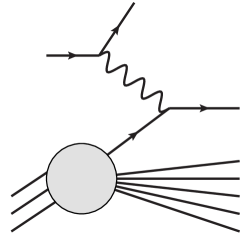
Figure 1: DIS process in the IMF: a virtual photon interacts with a pre-existing quark in the target.

In QCD one cannot calculate cross sections exactly. Instead, one arranges the calculations in a perturbative series assuming a small value for the coupling constant. When the scattering process studied involves QCD bound states, as is the case for DIS, one needs to separate the part of the process that can be described using weak coupling from the nonperturbative hadronic physics. The latter must then be parametrized by some functions of appropriate kinematical variables which must ultimately be obtained from experimental data or, in principle, from lattice calculations. A priori, there is no unique way to decide what are the best degrees of freedom to describe the nonperturbative part of the process. Different scattering processes or different kinematical regimes might be more optimally described using a different language. In order for the theory to have predictive power, the nonperturbative description should be as universal as possible. This means that the same degrees of freedom can be used in descriptions of different processes, e.g. measured in one process to calculate a genuine prediction for the cross section of another. It is also helpful, if not strictly speaking necessary, for the description to be related to a simple physical picture of the nonperturbative QCD bound state. A cross section is naturally a Lorentz invariant quantity and as such independent of the frame in which one decides to view the process. The microscopic degrees of freedom describing a QCD bound state can, however, be very different in different Lorentz frames. These different ways of viewing the nonperturbative structure of the bound state can be naturally adapted to very different schemes of organizing perturbative QCD calculations. This is indeed the case for the Infinite Momentum Frame (IMF) and the Target Rest Frame (TRF) (more appropriately the dipole frame) that we will describe in the following. Both are used to organize QCD calculations into perturbatively calculable parts, a nonperturbative input and weak coupling renormalization group equations describing the dependence of the nonperturbative input on some kinematical variable. Both have their advantages and disadvantages and are applicable for partially overlapping sets of scattering processes and kinematical regimes.

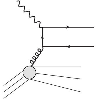
Figure 2: Higher order DIS process in the IMF: a virtual photon interacts with gluon via a quark-antiquark pair.

The usual perturbative QCD description of a DIS process is based on the collinear factorization formalism. The most natural physical picture in this case is the one in the IMF, where the proton moves at a very high energy. The relevant degrees of freedom in the proton are then quasi-free partons, quarks and gluons. The partons are collinear, i.e. they share a fraction $x=k^{+}/P^{+}$ of the longitudinal momentum (more precisely $+$-momentum) of the proton, but have a very small transverse momentum ${k_{T}}$. According to a simple uncertainty argument the (light cone) lifetime $\Delta x^{+}\sim 1/k^{-}=2k^{+}/{k_{T}}^{2}$ of these fluctuations is long compared to the resolution scale of the virtual photon, $\Delta x^{+}\sim 1/q^{-}\sim k^{+}/Q^{2}$. Thus the process can be viewed as a virtual photon instantaneously measuring the partonic content of the proton; to leading order just the quark distribution, see Fig. 1. Using light cone quantization, one can relate the cross section to the Fock state decomposition of the proton.

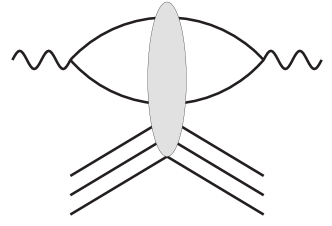
Figure 3: Leading order DIS process in the dipole picture: the virtual photon splits into a quark-antiquark pair, which interacts with the target.

To leading order in perturbation theory, the virtual photon only measures the quark number density in the target proton, see Fig. 1. QCD dynamics is probed in the collinear picture when one goes beyond leading order, e.g. in the process shown in Fig. 2. The degrees of freedom used to parametrize the nonperturbative physics of the proton are number densities of quarks and gluons, i.e. parton distribution functions (PDF’s). By extracting the leading large transverse momentum $Q^{2}$ behavior of the higher order diagrams such as Fig. 2, one can derive the DGLAP renormalization equations, which describe the dependence of these PDF’s on the external virtuality $Q^{2}$. The kinematical regime of validity of the decription for sufficiently inclusive processes is very broad; the longitudinal momentum fraction $x$ can be arbitrary as long as the momentum scale $Q^{2}$ is large enough.

Now let us look at the same process in a different frame where the target proton moves slowly, but the virtual photon has a large momentum $q^{+}$. Now, according to exactly the same kinematical argument as above, quantum fluctuations in the virtual photon exist on a much longer timescale than the interaction. They are then instantaneously struck by the color fields in the target proton. During this short interaction time the structure of the probe $\gamma^{*}$ is frozen. A natural method to understand this process is to light cone quantize the virtual photon. Since it is a clean and controlled object and not a complicated QCD bound state, the light cone quantization part of the calculation is purely perturbative. The nonperturbative object describing the target, on the other hand, is its scattering amplitude with the probe. The microscopical description of the target naturally associated with this picture is as a classical strong color field. Since the probe has a high energy, its interaction with this field can be calculated using the eikonal approximation.

Figure 4: Next to leading order DIS process in the dipole picture: the virtual photon state also has a quark-antiquark-gluon component.

The lowest nontrivial component in the $\gamma^{*}$ state that can interact with a target color field is a quark-antiquark dipole, Fig. 3. As in the collinear picture, QCD dynamics comes in when one moves to higher order in perturbation theory. In this case the perturbative expansion is the one describing the virtual photon, and the NLO correction involves the inclusion of an additional gluon in the virtual photon state, as depicted in Fig. 4. At least in the large $\href{http://www-spires.slac.stanford.edu/spires/find/hep/www?j=NUCIA\%2C$\%2Ci}{{\it Nuovo Cim.\ }{\bf$} (l) i}mit,ormoregenerallyusingamoreexplicitmodelforthescattering,e.g.theclassicalfieldpicture,thescatteringamplitudeofthe$q¯qg$statecanberelatedtothatoftheoriginaldipole.Theintegrationoverthephasespaceoftheadditionalgluonyieldsacorrectiontothecrosssectionoftheoriginaldipolethatisenhancedbyalargelogarithmoftheenergy$W^2$.Theselogarithmscanthenberesummedintoarenormalizationgroupequation:BK~{}\cite[cite]{[\@@bibref{}{Balitsky:1995ub,Kovchegov:1999yj}{}{}]}orJIMWLK~{}\cite[cite]{[\@@bibref{}{Jalilian-Marian:1997xn,Jalilian-Marian:1997jx,Jalilian-Marian:1997gr,Jalilian-Marian:1997dw,JalilianMarian:1998cb,Iancu:2000hn,Iancu:2001md,Ferreiro:2001qy,Iancu:2001ad,Weigert:2000gi,Mueller:2001uk}{}{}]}thatdescribesthedependenceofthescatteringamplitudeontheenergy.TheprocedureiscompletelyanalogoustothephysicsofDGLAP,with$ln1/x$playingtheroleof$lnQ^2$asthelargelogarithmresummedandthescatteringamplitudetheroleofthePDF^{\prime}sasthefunctiondescribingthetarget.Thedownsideofthispictureisthatitisonlyapplicableatsmall$x$,with$Q^2$nottoolargebutlargeenoughforthecouplingtobeweak.Buttocompensateforthisthereareseveraladvantages.Sinceoneisworkingdirectlywiththeimaginarypartoftheforwardelasticscatteringamplitude,i.e.thetotaldipole-targetcrosssection,implementingunitarityconstraintsisstraighforwardandtransparent.Thesameamplitudeisalsoprobedinelasticprocesses,i.e.diffractiveDIS,whichenhancesthepredictivepoweroftheframework.Thisshouldbecontrastedwithcollinearperturbationtheory,wherediffractivePDF^{\prime}sareusuallyfittodataindependentlyfromtheinclusiveones.Also,sinceoneisnotcountinggluonsinthetargetbuttreatingthemcoherentlyasacolorfield,theformalismismuchmorenaturallysuitedtodescribingthenonlinearphysicsofgluonsaturation.\par$

2.2 Gluon saturation

The physical picture of renormalization group evolution in the collinear framework is one of a cascade, where partons split by gluon emission and pair creation. As the virtuality $Q^{2}$ or energy $\sim 1/x$ increases, there is phase space for more of these splittings, and the number of partons grows. At some point in the cascade it is possible that the phase space density of gluons is large enough for also mergings of gluons to become important. We can parametrically estimate when this happens using the following simple argument [14]. We can assume, by the uncertainty principle, that one gluon accupies an area $\sim 1/Q^{2}$ in the tranverse plane. The number of these gluons per unit rapidity in a proton of area $\pi R_{p}^{2}$ is given by the gluon distribution $xG(x,Q^{2})$. Thus the number of gluons in a cell of size $1/Q^{2}$ is given by the gluon density times the area of the cell $\sim(xG(x,Q^{2})/\pi R_{p}^{2})\times(1/Q^{2})$. For gluon mergings to be important they must overlap enough to pay the price of the coupling $\alpha_{\mathrm{s}}$ in the probability for merging. This leads to the estimate that the gluon mergings become important when $xG(x,Q^{2})/(Q^{2}\pi R_{p}^{2})\gtrsim 1/\alpha_{\mathrm{s}}$. The $x$-dependent value of the characteristic transverse momentum scale at which this happens is known as the saturation scale $Q_{\textnormal{s}}$; it is the solution of the equation

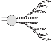
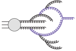
Figure 5: Linear and nonlinear cascade of gluons

$$\pi R_{p}^{2}Q_{\textnormal{s}}^{2}\sim\alpha_{\mathrm{s}}xG(x,Q_{\textnormal{s}}^{2}).$$ (1)

This equation is naturally an order of magnitude estimate, and the exact numerical value of a characteristic momentum scale depends on the precise definition. We will argue in the following that it is more natural to give such a definition in the dipole picture. Diagrammatically this transition from a cascade of pure splittings to one which also includes mergings could be illustrated by something like Fig. 5. In practice it is difficult to work quantitatively with gluon merging diagrams of the kind sketched in Fig. 5 (however, for an interesting attempt to introduce saturation into a Monte Carlo cascade see [15]). Thus the IMF collinear picture is not very convenient for understanding saturation quantitatively. It is also not clear whether the chosen degree of freedom, a number density of gluons, is conceptionally meaningful in a regime of important nonlinear interactions between them.

In the dipole picture the same phenomenon of parton saturation appears in a very different way. The target proton is described by a dimensionless (imaginary part of the forward elastic) scattering amplitude ${\mathcal{N}}$, which is related to the total dipole-target cross section by the optical theorem $\sigma=2\int\,\mathrm{d}^{2}{\mathbf{b}_{T}}{\mathcal{N}}$. The amplitude naturally varies between no interaction ${\mathcal{N}}=0$ and total absorption, i.e. the black disk limit ${\mathcal{N}}=1$ (in principle unitarity allows values up to ${\mathcal{N}}=2$). We are working in the eikonal approximation where the size of the dipole $r\sim 1/Q$ stays fixed during the interaction. Since a dipole of size $r=0$ is a color neutral object and should not interact in QCD, we know that ${\mathcal{N}}(r=0)=0$. For small enough dipoles the scattering should be weak and dominated by the perturbatively leading process of two-gluon exchange. Indeed one has

$$\sigma\sim 2\pi R_{p}^{2}\mathcal{N}(r)\sim\alpha_{\mathrm{s}}r^{2}xG\left(x,Q^{2}\sim 1/r^{2}\right)\quad\textnormal{ for }\quad r\to 0.$$ (2)

Now we can immediately see that the perturbative two-gluon exchange approximation cannot remain valid for arbitrarily large dipoles, i.e. small $Q^{2}$. Some mechanism involving multiple gluon ecxhanges must begin to be important when ${\mathcal{N}}\sim\alpha_{\mathrm{s}}r_{\textnormal{s}}^{2}xG(x,Q^{2}\sim 1/r_{\textnormal{s}}^{2})/(\pi R_{p}^{2})\sim 1$. With the identification $Q_{\textnormal{s}}=1/r_{\textnormal{s}}$ this is exactly the same saturation condition that we obtained previously in Eq. (1). The difference is that now the phenomenon does not appear to follow from nonlinear gluon dynamics. Instead it is required by unitarity and must, and easily can, be built into the formalism used. This is the case in the CGC framework, and in particular for the BK and JIMWLK equations. In practice this is done by assuming that the target is described by a strong color field, with which the quark and antiquark in the dipole interact eikonally by picking up an SU($\href{http://www-spires.slac.stanford.edu/spires/find/hep/www?j=NUCIA\%2C$\%2CW}{{\it Nuovo Cim.\ }{\bf$} ()) W}ilsonline\begin{equation}V=\mathbb{P}\exp\left\{-ig\int\!\!\,\mathrm{d}x^{+}A^{-}\right\}.\end{equation}ThedipoleamplitudethenturnsouttobeacorrelationfunctionoftwooftheseWilsonlines\begin{equation}{\mathcal{N}}({\mathbf{r}_{T}}={\mathbf{x}_{T}}-{\mathbf{y}_{T}})=1-\frac{1}{\href{http://www-spires.slac.stanford.edu/spires/find/hep/www?j=NUCIA\%2Cmissing\%2Cmissing}{{\it Nuovo Cim.\ }{\bf missing} (missing) missing}}\bigg{<}\,\mathrm{Tr}\,V^{\dagger}({\mathbf{x}_{T}})V({\mathbf{y}_{T}})\bigg{>},\end{equation}automaticallysatisfyingtherequirements$N(r=0)=0$and$N(r→∞)=1$(sinceatlargeseparationstheWilsonlinesareuncorrelatedandaverageseparatelytozeroforstrongfields).\par$

3 NLO theory

3.1 Evolution equations

 

Figure 6: Diagrams needed to derive the BK equation.

As discussed above, by including one additional gluon to the dipole (see Fig. 6), relating the $q\bar{q}$ and $q\bar{q}g$ cross sections to each other using the large $\href{http://www-spires.slac.stanford.edu/spires/find/hep/www?j=NUCIA\%2C$\%2Ce}{{\it Nuovo Cim.\ }{\bf$} (m) e}anfieldlimitandpickinguptheleadinglogarithmof$x$fromtheintegrationoverthephasespaceofthegluononecanderivetheleadingorderBKequationforthe$y=ln1/x$-dependenceofthescatteringamplitude$N$:\begin{equation}\partial_{y}\mathcal{N}({\mathbf{r}_{T}})=\frac{\alpha_{\mathrm{s}}\href{http://www-spires.slac.stanford.edu/spires/find/hep/www?j=NUCIA\%2Cmissing\%2Cmissing}{{\it Nuovo Cim.\ }{\bf missing} (missing) missing}}{2\pi^{2}}\int\,\mathrm{d}^{2}{\mathbf{r}^{\prime}_{T}}\frac{{\mathbf{r}_{T}}^{2}}{{\mathbf{r}^{\prime}_{T}}^{2}\left({\mathbf{r}^{\prime}_{T}}-{\mathbf{r}_{T}}\right)^{2}}\left[\mathcal{N}\left({\mathbf{r}^{\prime}_{T}}\right)+\mathcal{N}\left({\mathbf{r}_{T}}-{\mathbf{r}^{\prime}_{T}}\right)-\mathcal{N}\left({\mathbf{r}^{\prime}_{T}}\right)\mathcal{N}\left({\mathbf{r}_{T}}-{\mathbf{r}^{\prime}_{T}}\right)-\mathcal{N}\left({\mathbf{r}_{T}}\right)\right].\end{equation}Inthelinearlimit(droppingthe$N^2$-term)thisreducestotheLOBFKLequation.TheBFKLequationhasbeenknowntoNLOaccuracyforsometime\cite[cite]{[\@@bibref{}{Fadin:1996nw,Fadin:1998py,Ciafaloni:1998gs}{}{}]}.AttheNLOlevelonestartsalsopickinguplargelogarithmsoftransversemomenta,whichweresubsequentlyresummedinMellinspace~{}\cite[cite]{[\@@bibref{}{Salam:1998tj,Ciafaloni:1999yw,Altarelli:1999vw,Ciafaloni:2003rd}{}{}]}inordertogetameaningfulresult.TheNLOversionofthenonlinearBKequation~{}\cite[cite]{[\@@bibref{}{Balitsky:2008zza}{}{}]}(seealsotheequation~{}\cite[cite]{[\@@bibref{}{Balitsky:2014mca}{}{}]}forthebaryonoperator)hasalsobeenknownforseveralyears.Afullnumericalsolutionofthisequation,was,however,performedonlyveryrecently~{}\cite[cite]{[\@@bibref{}{Lappi:2015fma}{}{}]}(see,however,previousnumericalstudies~{}\cite[cite]{[\@@bibref{}{Avsar:2011ds}{}{}]}).Ascouldbeexpected,itsuffersfromthesameproblemswithlargetransverselogarithmsasNLOBFKL.Resummingtheminthecaseofthenonlinearequationrequires,however,differentmethodsthatareonlynowbeingdeveloped~{}\cite[cite]{[\@@bibref{}{Iancu:2015joa,Iancu:2015vea}{}{}]}.AtthetimeoftheDIS2015conference,thestateoftheartforphenomenologicalapplicationsisstilltheleadingorderBKequation,supplementedwithrunningcouplingcorrections.\par TheBKequationusesamean-fieldapproximation(replacing$¡^D^D ¿→¡^D¿¡^D ¿$,where$^D=1Nuovo Cim. missing (missing) missing  Tr   V^†V$isthedipoleoperator)toclosetheequation.WithoutthisapproximationoneobtainsamoregeneralinfinitehierarchyofequationsthatcouplesexpectationvaluesofdifferentproductsofWilsonlines.Thishierarchycanbeequivalentlywrittenasarenormalizationgroupequationforthe\emph{probability distribution}ofWilsonlines,andisknownastheJIMWLKequation.WhiletheNLOJIMWLKequationcannotdirectlybereadofffromtheNLOBKequation,theloopintegralsrequiredinderivingthetwoaremostlythesame.ThishasveryrecentlymadeitpossibletoderivetheNLOJIMWLKequation~{}\cite[cite]{[\@@bibref{}{Balitsky:2013fea,Kovner:2013ona}{}{}]},relyingheavilyontheseearlierresults.\par$

3.2 Forward particle production in pA

 

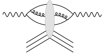
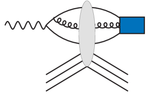
Figure 7: Left: A contribution to the NLO impact factor for DIS. Right: A contribution to NLO exclusive vector meson production.

For a full NLO calculation of a physical cross section the evolution equations by themselves are not enough. One must also calculate the parts of the process without a large resummed logarithm to NLO accuracy. For the case of DIS this means the full calculation of diagrams such as the one in Fig. 7, where the leading high energy logarithm gives the LO evolution equation and the remainder is a part of the NLO ”impact factor”. This has been done in two separate papers [31, 32] using a slightly different formalism. The consistency of these two results with each other is yet to be confirmed, and neither of them has yet been applied to practical phenomenology. A similar calculation, involving the modeling of the $q\bar{q}g$ state in a vector meson wavefunction (see Fig. 7) would be required for exclusive vector meson production.

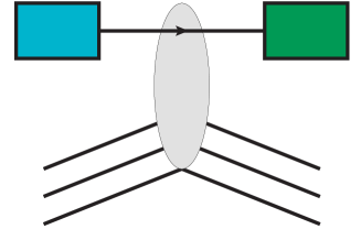
Figure 8: Forward particle production at leading order.

While progress in NLO DIS phenomenology has been slower, there has been much activity recently on calculating particle production in forward proton-nucleus collisions to NLO. Here the physical picture (see Fig. 8) starts from a high-$x$ quark or gluon from the proton, described using a conventional collinear PDF. The quark passes through the strong color field of the target nucleus, acquiring transverse momentum from the intrinsic ${k_{T}}$ of the small-$x$ gluons in the target and finally fragments into hadrons. The fragmentation can be described by conventional fragmentation functions, but the interaction with the target is given by the same Wilson line as the quark and antiquark in DIS, Eq. (3). When the eikonal quark-target scattering amplitude is squared, one obtains a cross section which is essentially given by just the Fourier-transform of the (DIS) dipole cross section (4).

 

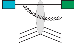
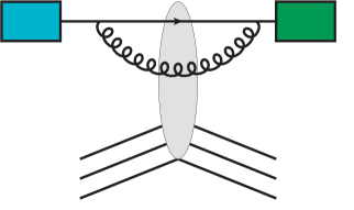
Figure 9: Real (left) and virtual (right) NLO corrections to quark production in forward proton-nucleus collisions.

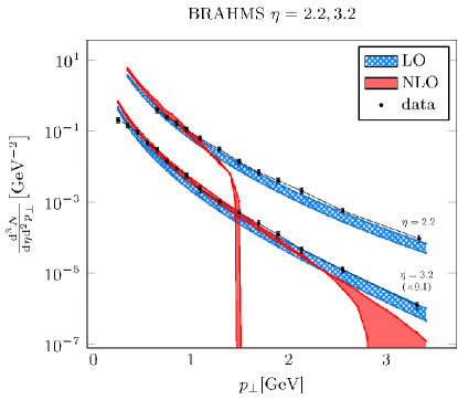
Figure 10: LO and NLO single inclusive cross sections from [33] compared to BRAHMS data.

At NLO accuracy one needs to consider the one loop corrections, e.g. the ones shown in Fig. 9. Some years back Chirilli et. al. [34, 35] demonstrated that, as expected, the appropriate logs of $x$ and $Q^{2}$ in these contributions can be factorized into the BK evolution of the target amplitude and the DGLAP evolution of the probe PDF and the fragmentation function. Unfortunately attempts to apply these results led to very large NLO corrections that, at high ${p_{T}}$, made the total cross section negative [33] (see Fig. 10). Several authors have tried to understand this problem [36, 37, 38, 39] and propose solutions. While some progress has indeed been made on the matter, it seems fair to say that the question of NLO particle production is still unsettled, and still an area of active study.

3.3 Transverse momentum and spin

The conventional operator definition for the transverse momentum dependent (TMD) gluon distribution is

$$xG(x,{\mathbf{k}_{T}})=\int\frac{\,\mathrm{d}x^{-}\,\mathrm{d}^{2}{\mathbf{x}_{T}}}{(2\pi)^{3}P^{+}}e^{ixP^{+}x^{-}-i{\mathbf{k}_{T}}\cdot{\mathbf{x}_{T}}}\langle P|F^{+i}(x^{-},{\mathbf{x}_{T}})\mathcal{L}F^{+i}(0)|P\rangle.$$ (6)

Since the operator is nonlocal, the two insertions of the field strength tensor $F^{i+}$ have to be connected by a gauge link $\mathcal{L}$, which follows a path that can be different for different processes. With a more general Lorentz index structure one can also write down similar expressions for spin dependent distributions. A major advance in the field in recent years has been to understand [40, 41, 42, 43, 44] how these different TMD distributions can, at small $x$, be expressed in terms of the Wilson lines (3). In the conventional perturbation theory framework the different distributions must be separately fit to separate experimental data. Being able to express them all in terms of the same Wilson line greatly enhances the universality and predictive power of the theory. In the CGC framework one can, for example, use only $F_{2}$ structure function data to fit the initial conditions for the BK evolution of the distribution of Wilson lines. These can then be used to calculate various TMD and spin distributions without any additional experimental data.

One example of such a TMD distribution is the linearly polarized gluon distribution [45]. Experimentally it is probed in dijet production in DIS, where the dependence of the cross sections on the azimuthal angle between the total and relative transverse momenta of the two jets (i.e. the angle between ${\mathbf{k}_{T1}}+{\mathbf{k}_{T2}}$ and ${\mathbf{k}_{T1}}-{\mathbf{k}_{T2}}$, where ${\mathbf{k}_{T1}}$ and ${\mathbf{k}_{T2}}$ are the transverse momenta of the jets). Measurements of multiparticle azimuthal correlations are a subject of much interest also in heavy ion collisions, where they are created in abundance by collective effects in the plasma. Indeed, starting from a coordinate space asymmetric initial distribution of matter as in a noncentral heavy ion collision, hydrodynamical flow generates strong anisotropies in momentum space due to the anisotropy of pressure gradients. The similar experimental signature of these very different physical effects, collective flow in QCD matter and polarization and correlation effects that are present already in DIS, makes the interpretation of multiparticle correlations measurements in proton-proton and proton-nucleus collisions very challenging.

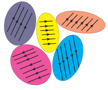
Figure 11: Color fields seen by dilute probe.

In the CGC picture, the mechanism for generating azimuthal correlations whithout collective final state effects has a very intuitive physical interpretation, which is easiest to describe in the case of a dilute object (dipole, forward proton) colliding with the dense color field [46]. The picture of particle production in this case is that of the particles from the probe passing through target that consists of domains of transverse color electric field (Fig. 11). The size of these domains in coordinate space is $\sim 1/Q_{\textnormal{s}}$, which corresponds to the target consisting of gluons with ${k_{T}}\sim Q_{\textnormal{s}}$. Particles from the probe that pass through the same domain in the target and that have the same color experience the same color electric field and are deflected in the same direction. This naturally leads to an angular correlation between these particles, and has been put forward [47, 48, 49, 50] as an at least partial explanation for many such correlation phenomena seen in proton-proton and proton-nucleus collisions.

4 Exclusive processes

Let us finally move to a topic where recent progress has been more experimentally driven, namely exclusive processes and in particular vector meson production. One of the strengths of the dipole picture is that the cross section is given by the square of the same elastic dipole-target scattering amplitude that determines the total cross section. This enables a direct relation between inclusive diffraction and the total cross section [51, 52, 53]. The additional ingredient needed for the description of exclusive vector meson production is the transition matrix element from the dipole to the vector meson bound state. This leads one to focus attention on heavy quark mesons, whose bound state properties can to some degree be understood perturbatively. In light cone quantization this information is expressed in terms of the so called vector meson (light cone) “wavefunction” (see Fig. 12).

Exclusive processes can provide important constraints for models of small $x$ gluons. However, due to the additional complication of the vector meson bound states, systematical studies are needed as a function of $x$, $Q^{2}$ (see e.g. [54]), vector meson species and nuclear mass number.

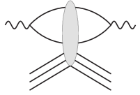
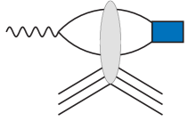
Figure 12: Total DIS cross section via the optical theorem (left) and the amplitude for exclusive vector meson production (right). The circled blob is the common amplitude, while the box surrounded by the dashed circle is the vector meson light cone wavefunction.

While waiting for an Electron-Ion Collider to explore the full parameter space, the nuclear mass number dependence can be addressed in the photoproduction limit $Q^{2}=0$ by ultraperipheral nucleus-nucleus collisions (UPC’s) at the LHC and at RHIC. The idea with UPC is to use the high electric charge of the fully ionized nucleus as a source of real photons. By triggering on events with no hadronic activity (besides the vector meson) one restricts the impact parameter to be beyond the range of the strong interaction; hence the term ultraperipheral. Using the equivalent flux of Weizsäcker-Williams photons from the ion one can relate the measured cross section to the photon-nucleus (or photon-proton) cross section.

Experimental studies of exclusive vector meson production are often portrayed as measurements of the nuclear gluon distribution. This interpretation is based on the formula that relates the exclusive vector meson cross section to the target gluon distribution as

$$\left.\frac{\,\mathrm{d}\sigma^{\gamma^{*}H\to VH}}{\,\mathrm{d}t}\right|_{t=0}=\frac{16\pi^{3}\alpha_{\mathrm{s}}^{2}\Gamma_{ee}}{3\alpha_{\textnormal{em}}M_{V}^{5}}\left[xg(x,Q^{2}=M_{V}^{2})\right]^{2}.$$ (7)

This equation is in fact [55] the small $r$ limit of the dipole model calculation, where the dipole cross section is related to the gluon distribution as in Eq. (2) and the wavefunction is reduced to its behavior around the origin, where it can be related to the electromagnetic decay width of the meson $\Gamma_{ee}$. Some of the theory calculations are indeed based on this formula, usually supplemented with phenomenological corrections for the normalization. In the CGC picture, however, it is natural to go beyond the small-$r$ limit and include the full integral over different size dipoles.

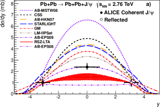
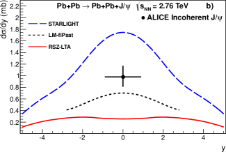
Figure 13: ALICE results for coherent $J/\Psi$ production compared to theoretical models, from [56]

In the case of nuclear targets one distinguishes two classes of events: coherent, where the nucleus stays intact in its ground state, and incoherent, where it breaks up, but only into color neutral protons and neutrons, preserving the rapidity gap characteristic of diffractive events. Coherent events dominate for small momentum transfers to the target $|t|\sim 1/R_{A}^{2}$, where $R_{A}$ is the nuclear radius. For $|t|\sim 1/R_{p}^{2}$, which is the typical momentum transfer for exclusive $ep$ events, the incoherent process dominates. Even here, however, the cross section is very much affected by nuclear effects, being suppressed by a factor $\sim 3$ [57] compered to $A$ times the nucleon cross section. This suppression can be understood as arising from a “survival probability”, where the (virtual) photon, after interacting elastically with one nucleon, must not interact inelastically with spectator nucleons to preserve the rapidity gap. The ALICE collaboration distinguishes between these two classes largely based on the transverse momentum of the vector meson which, for $Q^{2}=0$, is the same as the recoil momentum of the nucleus. The coherent cross section is related to the average gluon density in the nucleus, while the incoherent one directly measures the fluctuations [57]. This interpretation is very implicit in the SARTRE event generator [58]. Thus the incoherent data provides an important constraint on the fluctuating nuclear geometry that has become an important aspect of interpretations of heavy ion collisions, and deserves to be better addressed by the theory community.

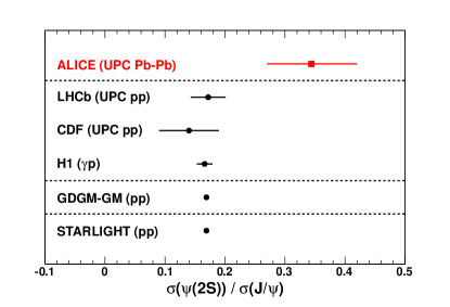
Figure 14: Ratio of $J/\Psi$ to $\Psi(2S)$ photoproduction cross sections from $\gamma$-proton collisions compared to the ALICE result from $\gamma$-nucleus collisions [59].

Figure 13 shows first results on $J/\Psi$ production from ALICE [56, 60] compared to theory calculations. Results have also been published by LHCb [61] ($\gamma$-proton collisions) and CMS [62] ($\gamma$-nucleus collisions). A particularly interesting result from ALICE is on the $\Psi(2S)$ to $J/\Psi$ cross section ratio (see Fig. 14), which is measured to be approximately twice as large as in $\gamma p$ collisions. In the dipole picture the cross section of the $2S$ state is suppressed with respect to the $1S$ state due to the “node effect”, i.e. a cancellation between different sign parts in the excited state meson wavefunction. Since the increased saturation scale diminishes the relative importance of the large-$r$ cross section, this node effect cancellation is naturally weaker for nuclei than for protons. In practice, however, it is difficult to see how the effect could become as large as indicated by the ALICE data. With many of the measurements still statistics limited, we can expect many more such interesting results from the future LHC runs.

5 Conclusions

In conclusion, we have here discussed some recent focus areas in small-$x$ physics, concentrating in particular on developments in the nonlinear gluon saturation regime. On the theory side, there is a systematical effort to push calculations to NLO accuracy. In spite of the recent progress there is still work to do to understand the interplay of small $x$ and large $Q^{2}$ logarithms at the NLO level. Another related area have been connections between the saturation formalism and that of TMD gluon distributions. Also here, the understanding of the formal theory side has improved significantly, but there is still much to do to turn these ideas into precision phenomenology. We have also discussed recent experimental progress, in particular with exclusive photoproduction of vector mesons at the LHC.

Acknowledgements

This work has been supported by the Academy of Finland, projects 267321 and 273464. The author thanks K. J. Eskola for comments on the manuscript.

References

- [1] I. Balitsky, Operator expansion for high-energy scattering, Nucl. Phys. B463 (1996) 99 [arXiv:hep-ph/9509348].
- [2] Y. V. Kovchegov, Small-x F2 structure function of a nucleus including multiple pomeron exchanges, Phys. Rev. D60 (1999) 034008 [arXiv:hep-ph/9901281].
- [3] J. Jalilian-Marian, A. Kovner, L. D. McLerran and H. Weigert, The intrinsic glue distribution at very small x, Phys. Rev. D55 (1997) 5414 [arXiv:hep-ph/9606337 [hep-ph]].
- [4] J. Jalilian-Marian, A. Kovner, A. Leonidov and H. Weigert, The BFKL equation from the Wilson renormalization group, Nucl. Phys. B504 (1997) 415 [arXiv:hep-ph/9701284].
- [5] J. Jalilian-Marian, A. Kovner, A. Leonidov and H. Weigert, The Wilson renormalization group for low x physics: Towards the high density regime, Phys. Rev. D59 (1999) 014014 [arXiv:hep-ph/9706377].
- [6] J. Jalilian-Marian, A. Kovner and H. Weigert, The Wilson renormalization group for low x physics: Gluon evolution at finite parton density, Phys. Rev. D59 (1999) 014015 [arXiv:hep-ph/9709432].
- [7] J. Jalilian-Marian, A. Kovner, A. Leonidov and H. Weigert, Unitarization of gluon distribution in the doubly logarithmic regime at high density, Phys. Rev. D59 (1999) 034007 [arXiv:hep-ph/9807462].
- [8] E. Iancu, A. Leonidov and L. D. McLerran, Nonlinear gluon evolution in the color glass condensate. I, Nucl. Phys. A692 (2001) 583 [arXiv:hep-ph/0011241].
- [9] E. Iancu and L. D. McLerran, Saturation and universality in QCD at small x, Phys. Lett. B510 (2001) 145 [arXiv:hep-ph/0103032].
- [10] E. Ferreiro, E. Iancu, A. Leonidov and L. McLerran, Nonlinear gluon evolution in the color glass condensate. II, Nucl. Phys. A703 (2002) 489 [arXiv:hep-ph/0109115].
- [11] E. Iancu, A. Leonidov and L. D. McLerran, The renormalization group equation for the color glass condensate, Phys. Lett. B510 (2001) 133 [arXiv:hep-ph/0102009].
- [12] H. Weigert, Unitarity at small Bjorken x, Nucl. Phys. A703 (2002) 823 [arXiv:hep-ph/0004044 [hep-ph]].
- [13] A. H. Mueller, A simple derivation of the JIMWLK equation, Phys. Lett. B523 (2001) 243 [arXiv:hep-ph/0110169].
- [14] A. H. Mueller and J.-w. Qiu, Gluon recombination and shadowing at small values of x, Nucl. Phys. B268 (1986) 427.
- [15] E. Avsar, G. Gustafson and L. Lonnblad, Small-x dipole evolution beyond the large- limit, JHEP 01 (2007) 012 [arXiv:hep-ph/0610157 [hep-ph]].
- [16] V. S. Fadin and L. Lipatov, Next-to-leading corrections to the BFKL equation from the gluon and quark production, Nucl. Phys. B477 (1996) 767 [arXiv:hep-ph/9602287 [hep-ph]].
- [17] V. S. Fadin and L. Lipatov, BFKL pomeron in the next-to-leading approximation, Phys. Lett. B429 (1998) 127 [arXiv:hep-ph/9802290 [hep-ph]].
- [18] M. Ciafaloni and G. Camici, Energy scale(s) and next-to-leading BFKL equation, Phys. Lett. B430 (1998) 349 [arXiv:hep-ph/9803389 [hep-ph]].
- [19] G. Salam, A resummation of large subleading corrections at small x, JHEP 9807 (1998) 019 [arXiv:hep-ph/9806482 [hep-ph]].
- [20] M. Ciafaloni, D. Colferai and G. Salam, Renormalization group improved small x equation, Phys. Rev. D60 (1999) 114036 [arXiv:hep-ph/9905566 [hep-ph]].
- [21] G. Altarelli, R. D. Ball and S. Forte, Resummation of singlet parton evolution at small x, Nucl. Phys. B575 (2000) 313 [arXiv:hep-ph/9911273 [hep-ph]].
- [22] M. Ciafaloni, D. Colferai, G. Salam and A. Stasto, Renormalization group improved small x Green’s function, Phys. Rev. D68 (2003) 114003 [arXiv:hep-ph/0307188 [hep-ph]].
- [23] I. Balitsky and G. A. Chirilli, Next-to-leading order evolution of color dipoles, Phys. Rev. D77 (2008) 014019 [arXiv:0710.4330 [hep-ph]].
- [24] I. Balitsky and A. V. Grabovsky, NLO evolution of 3-quark Wilson loop operator, JHEP 01 (2015) 009 [arXiv:1405.0443 [hep-ph]].
- [25] T. Lappi and H. Mäntysaari, Direct numerical solution of the coordinate space Balitsky-Kovchegov equation at next to leading order, Phys. Rev. D91 (2015) 074016 [arXiv:1502.02400 [hep-ph]].
- [26] E. Avsar, A. Stasto, D. Triantafyllopoulos and D. Zaslavsky, Next-to-leading and resummed BFKL evolution with saturation boundary, JHEP 1110 (2011) 138 [arXiv:1107.1252 [hep-ph]].
- [27] E. Iancu, J. D. Madrigal, A. H. Mueller, G. Soyez and D. N. Triantafyllopoulos, Collinearly-improved BK evolution meets the HERA data, arXiv:1507.03651 [hep-ph].
- [28] E. Iancu, J. Madrigal, A. Mueller, G. Soyez and D. Triantafyllopoulos, Resumming double logarithms in the QCD evolution of color dipoles, arXiv:1502.05642 [hep-ph].
- [29] I. Balitsky and G. A. Chirilli, Rapidity evolution of Wilson lines at the next-to-leading order, Phys. Rev. D88 (2013) 111501 [arXiv:1309.7644 [hep-ph]].
- [30] A. Kovner, M. Lublinsky and Y. Mulian, Jalilian-Marian, Iancu, McLerran, Weigert, Leonidov, Kovner evolution at next to leading order, Phys. Rev. D89 (2014) 061704 [arXiv:1310.0378 [hep-ph]].
- [31] I. Balitsky and G. A. Chirilli, Photon impact factor in the next-to-leading order, Phys. Rev. D83 (2011) 031502 [arXiv:1009.4729 [hep-ph]].
- [32] G. Beuf, NLO corrections for the dipole factorization of dis structure functions at low x, Phys. Rev. D85 (2012) 034039 [arXiv:1112.4501 [hep-ph]].
- [33] A. M. Stasto, B.-W. Xiao and D. Zaslavsky, Towards the test of saturation physics beyond leading logarithm, Phys. Rev. Lett. 112 (2014) 012302 [arXiv:1307.4057 [hep-ph]].
- [34] G. A. Chirilli, B.-W. Xiao and F. Yuan, One-loop factorization for inclusive hadron production in pA collisions in the saturation formalism, Phys. Rev. Lett. 108 (2012) 122301 [arXiv:1112.1061 [hep-ph]].
- [35] G. A. Chirilli, B.-W. Xiao and F. Yuan, Inclusive hadron productions in pA collisions, Phys. Rev. D86 (2012) 054005 [arXiv:1203.6139 [hep-ph]].
- [36] A. M. Staśto, B.-W. Xiao, F. Yuan and D. Zaslavsky, Matching collinear and small factorization calculations for inclusive hadron production in collisions, Phys. Rev. D90 (2014)no.~1 014047 [arXiv:1405.6311 [hep-ph]].
- [37] Z.-B. Kang, I. Vitev and H. Xing, Next-to-leading order forward hadron production in the small- regime: rapidity factorization, Phys. Rev. Lett. 113 (2014) 062002 [arXiv:1403.5221 [hep-ph]].
- [38] T. Altinoluk, N. Armesto, G. Beuf, A. Kovner and M. Lublinsky, Single-inclusive particle production in proton-nucleus collisions at next-to-leading order in the hybrid formalism, Phys. Rev. D91 (2015) 094016 [arXiv:1411.2869 [hep-ph]].
- [39] K. Watanabe, B.-W. Xiao, F. Yuan and D. Zaslavsky, Implementing the exact kinematical constraint in the saturation formalism, arXiv:1505.05183 [hep-ph].
- [40] F. Dominguez, C. Marquet, B.-W. Xiao and F. Yuan, Universality of unintegrated gluon distributions at small x, Phys. Rev. D83 (2011) 105005 [arXiv:1101.0715 [hep-ph]].
- [41] Y. V. Kovchegov and M. D. Sievert, Sivers function in the quasiclassical approximation, Phys. Rev. D89 (2014) 054035 [arXiv:1310.5028 [hep-ph]].
- [42] I. Balitsky and A. Tarasov, Rapidity evolution of gluon TMD from low to moderate , arXiv:1505.02151 [hep-ph].
- [43] P. Kotko, K. Kutak, C. Marquet, E. Petreska, S. Sapeta and A. van Hameren, Improved TMD factorization for forward dijet production in dilute-dense hadronic collisions, arXiv:1503.03421 [hep-ph].
- [44] Y. V. Kovchegov and M. D. Sievert, Calculating TMDs of an unpolarized target: Quasi-classical approximation and quantum evolution, arXiv:1505.01176 [hep-ph].
- [45] A. Metz and J. Zhou, Distribution of linearly polarized gluons inside a large nucleus, Phys. Rev. D84 (2011) 051503 [arXiv:1105.1991 [hep-ph]].
- [46] A. Kovner and M. Lublinsky, Angular correlations in gluon production at high energy, Phys. Rev. D83 (2011) 034017 [arXiv:1012.3398 [hep-ph]].
- [47] A. Dumitru, F. Gelis, L. McLerran and R. Venugopalan, Glasma flux tubes and the near side ridge phenomenon at RHIC, Nucl. Phys. A810 (2008) 91 [arXiv:0804.3858 [hep-ph]].
- [48] A. Dumitru, K. Dusling, F. Gelis, J. Jalilian-Marian, T. Lappi and R. Venugopalan, The ridge in proton-proton collisions at the LHC, Phys. Lett. B697 (2011) 21 [arXiv:1009.5295 [hep-ph]].
- [49] A. Dumitru and A. V. Giannini, Initial state angular asymmetries in high energy p+A collisions: spontaneous breaking of rotational symmetry by a color electric field and C-odd fluctuations, Nucl. Phys. A933 (2014) 212 [arXiv:1406.5781 [hep-ph]].
- [50] T. Lappi, Azimuthal harmonics of color fields in a high energy nucleus, Phys. Lett. B744 (2015) 315 [arXiv:1501.05505 [hep-ph]].
- [51] N. Nikolaev and B. G. Zakharov, Pomeron structure function and diffraction dissociation of virtual photons in perturbative QCD, Z. Phys. C53 (1992) 331.
- [52] H. Kowalski and D. Teaney, An impact parameter dipole saturation model, Phys. Rev. D68 (2003) 114005 [arXiv:hep-ph/0304189].
- [53] H. Kowalski, L. Motyka and G. Watt, Exclusive diffractive processes at HERA within the dipole picture, Phys. Rev. D74 (2006) 074016 [arXiv:hep-ph/0606272].
- [54] ZEUS collaboration, N. Kovalchuk, Charmonium production at HERA, PoS DIS2014 (2014) 187.
- [55] S. J. Brodsky, L. Frankfurt, J. Gunion, A. H. Mueller and M. Strikman, Diffractive leptoproduction of vector mesons in QCD, Phys. Rev. D50 (1994) 3134 [arXiv:hep-ph/9402283 [hep-ph]].
- [56] ALICE collaboration, E. Abbas et. al., Charmonium and pair photoproduction at mid-rapidity in ultra-peripheral Pb-Pb collisions at =2.76 TeV, Eur. Phys. J. C73 (2013) 2617 [arXiv:1305.1467 [nucl-ex]].
- [57] T. Lappi and H. Mäntysaari, Incoherent diffractive -production in high energy nuclear DIS, Phys. Rev. C83 (2011) 065202 [arXiv:1011.1988 [hep-ph]].
- [58] T. Toll and T. Ullrich, Exclusive diffractive processes in electron-ion collisions, Phys. Rev. C87 (2013) 024913 [arXiv:1211.3048 [hep-ph]].
- [59] ALICE collaboration, J. Adam et. al., Coherent (2S) photo-production in ultra-peripheral Pb-Pb collisions at = 2.76 TeV, arXiv:1508.05076 [nucl-ex].
- [60] ALICE collaboration, B. Abelev et. al., Coherent photoproduction in ultra-peripheral Pb-Pb collisions at TeV, Phys. Lett. B718 (2013) 1273 [arXiv:1209.3715 [nucl-ex]].
- [61] LHCb collaboration, R. Aaij et. al., Updated measurements of exclusive and (2S) production cross-sections in pp collisions at TeV, J. Phys. G41 (2014) 055002 [arXiv:1401.3288 [hep-ex]].
- [62] CMS collaboration, Photoproduction of the coherent accompanied by the forward neutron emission in ultra-peripheral PbPb collisions at 2.76 TeV, 2014. CMS-PAS-HIN-12-009.