On Consistency of Approximate Bayesian Computation

Abstract

Approximate Bayesian computation (ABC) methods have become increasingly prevalent of late, facilitating as they do the analysis of intractable, or challenging, statistical problems. With the initial focus being primarily on the practical import of ABC, exploration of its formal statistical properties has begun to attract more attention. The aim of this paper is to establish general conditions under which ABC methods are Bayesian consistent, in the sense of producing draws that yield a degenerate posterior distribution at the true parameter (vector) asymptotically (in the sample size). We derive conditions under which arbitrary summary statistics yield consistent inference in the Bayesian sense, with these conditions linked to identification of the true parameters. Using simple illustrative examples that have featured in the literature, we demonstrate that identification, and hence consistency, is unlikely to be achieved in many cases, and propose a simple diagnostic procedure that can indicate the presence of this problem. We also formally explore the link between consistency and the use of auxiliary models within ABC, and illustrate the subsequent results in the Lotka-Volterra predator-prey model.

Keywords: Bayesian consistency, likelihood-free methods, conditioning, auxiliary model-based ABC, ordinary differential equations, Lotka-Volterra model.

JEL Classification: C11, C15, C18

MSC2010 Subject Classification: 62F15, 62F12, 62C10

1 Introduction

The use of approximate Bayesian computation (ABC) methods in models with intractable likelihoods has gained increased momentum over recent years, extending beyond the original applications in the biological sciences. (See Marin et al., 2011, and Sisson and Fan, 2011, for recent reviews.). Whilst ABC evolved initially as a practical tool, attention has begun to shift to the investigation of its formal statistical properties, in particular as they relate to the choice of summary statistics on which the technique typically relies; see for example, Fearnhead and Prangle (2012), Gleim and Pigorsch (2013), Marin et al. (2014), Martin et al. (2014) and Martin et al. (2014).

The aim of this paper is to establish general conditions under which summary statistic-based ABC methods are Bayesian consistent, in the sense of producing draws that yield a degenerate distribution at the true parameter (vector) in the (sample size) limit. This aim is much broader than that underlying Martin et al. (2014), in which standard quasi-likelihood conditions were invoked to establish the Bayesian consistency of auxiliary model-based versions of ABC. In particular, we derive the conditions under which arbitrary summary statistics yield consistent inference, with these conditions linked to the identification of the true parameters in any particular instance. Using simple illustrative examples that have featured in the literature, we demonstrate that consistency is not achieved in many cases. This finding calls into doubt routine applications of the ABC method that are driven primarily by the convenience with which simple summary statistics can be computed, without further thought being given to the information content of those summaries.

Consistency by its very nature is more of a “thought experiment” than a practical feature of an estimation procedure. Nonetheless, consistency is a useful metric with which to gauge the output of a given statistical procedure. Following Diaconis and Freedman (1986), we argue that regardless of Bayesian bearing, that is, whether one is a “Classical” Bayesian (who believes in a “true but unknown parameter which is to be estimated from the data”) or a “Subjective” Bayesian (who does not believe in true models but, rather, thinks in terms of predictive distributions) consistency is important for verification and practical implementation of Bayesian procedures. That is, whilst consistency is a property that sits naturally within the Classical Bayesian paradigm, it can also be viewed as being important to Subjectivists. To wit, Blackwell and Dubins (1962) and Diaconis and Freedman (1986) argue that consistency can be viewed as a “merging of intersubjective opinions” and that consistency of the posterior implies that two separate subjective Bayesians with different prior beliefs will ultimately end up with similar predictive distributions.

In what follows, we only concern ourselves with the idea of consistency as it pertains to some true model that is known up to an unknown vector of parameters. In this setting Bayesian consistency means that any Bayesian method should yield increasingly accurate posterior inference as the sample size increases. While the theory of Bayesian consistency for likelihood-based Bayesian methods is now well documented, at least in the finite-dimensional parameter case, a thorough study on Bayesian consistency of so-called likelihood free methods, such as ABC, has yet to be undertaken. This represents an important gap in the literature, and is one we look to fill.

Bayesian consistency for posteriors based on finite-dimensional parameters is often derived under boundedness conditions for the underlying density function of the true model; see, for example, Le Cam (1953), Ibragimov and Has’minskii (1981), and Ghosal et al. (1995). In the ABC setting however, conditions based on the underlying density function are not useful since by the nature of the very problems to which ABC is applied, the underlying density is typically unknown in closed form. To this end, we derive a set of conditions on the summary statistics chosen within the ABC procedure that, when satisfied, ensure consistency of the posterior obtained from ABC. These conditions are similar in spirit to those seen in the literature on indirect inference (Gouriéroux, et al., 1993). Examples from the ABC literature are used to demonstrate how the aforementioned conditions can be verified in practice.

The paper proceeds as follows. In Section 2 we briefly outline the basic principles of ABC. In Section 3, we establish conditions under which ABC will be consistent for the unknown parameters, and simple examples that respectively do and do not satisfy these conditions are given. In Section 4 we then propose a practical technique for identifying, in any particular problem, when the conditions for consistency are (or are not) satisfied. The analysis in Sections 3 and 4 focuses on the typical application of ABC, whereby summary statistics are chosen that are deemed to contain some information about the parameters of the true model and, more often than not, are used to define a matching criterion that is a weighted function of sample moments. In Section 5 we couch the discussion in terms of a general criterion function, where the latter derives from an auxiliary model, and which may - but certainly does not need to - derive from the likelihood function of that approximating model. In Section 6 we pursue the matter of consistency when using ABC to conduct inference in systems of ordinary differential equations (ODEs), with the Lotka-Volterra system for predator and prey used for illustration, and demonstrate that a common method for obtaining ABC posterior estimates in this setting does not yield Bayesian consistent inference. Section 7 concludes. Proofs of two theorems and one corollary are provided in an appendix to the paper.

2 ABC: an Outline of the Basic Approach

Suppose we are interested in conducting Bayesian inference on a complex parametric model indexed by the unknown $p$-dimensional parameter $\mathbf{\theta}\in\mathbf{\Theta}$, $\mathbf{\Theta}\subset\mathbb{R}^{p}$ compact, and let $P_{\mathbf{\theta}}$ denote the family of probability measures induced by the model. Assume $P_{\mathbf{\theta}}$ admits a corresponding conditional density $p(\cdot|\mathbf{\theta})$ and assume we have $T$ observations on the stochastic process $y_{t}$, characterized by $p(\mathbf{y|\theta})$, with $\mathbf{y}=(y_{1},y_{2},...,y_{T})^{\prime}$ denoting the $T$-dimensional vector of observed data. The aim of ABC is to produce draws from an approximation to the posterior distribution of the unknown $\mathbf{\theta}$ given observed data $\mathbf{y}$,

$$p(\mathbf{\theta|y})\propto p(\mathbf{y|\theta})p(\mathbf{\theta}),$$

in the case where both the prior, $p(\mathbf{\theta})$, and the likelihood, $p(\mathbf{y|\theta})$, can be easily simulated. These draws are used, in turn, to approximate posterior quantities of interest, including marginal posterior moments, marginal posterior distributions and predictive distributions. The simplest (accept/reject) form of the algorithm (Tavaré et al., 1997, Pritchard et al., 1999) is detailed in Algorithm 1.

Algorithm 1 ABC algorithm

1:Simulate $\mathbf{\theta}^{i}$, $i=1,2,...,N$, from $p(\mathbf{\theta})$

2:Simulate $\mathbf{z}^{i}=(z_{1}^{i},z_{2}^{i},...,z_{T}^{i})^{\prime}$, $i=1,2,...,N$, from the likelihood, $p(\mathbf{.|\theta}^{i})$

3:Select $\mathbf{\theta}^{i}$ such that:

$$d\{\mathbf{\eta}(\mathbf{y}),\mathbf{\eta}(\mathbf{z}^{i})\}\leq\varepsilon,$$ (1)

where $\mathbf{\eta}(\mathbf{\cdot})$ is a (vector) statistic, $d\{\cdot,\cdot\}$ is a distance function (or metric), and the tolerance level $\varepsilon$ is chosen as small as the computing budget allows.

Algorithm 1 thus samples $\mathbf{\theta}$ and $\mathbf{z}$ from the joint posterior:

$$p_{\varepsilon}(\mathbf{\theta},\mathbf{z|\eta(y)})=\frac{p(\mathbf{\theta})p(\mathbf{z|\theta})\mathbb{I}_{\varepsilon}[\mathbf{z}(\mathbf{\theta})]}{\textstyle\int_{\mathbf{\Theta}}\int_{\mathbf{z}}p(\mathbf{\theta})p(\mathbf{z|\theta})\mathbb{I}_{\varepsilon}[\mathbf{z}(\mathbf{\theta})]d\mathbf{z}d\mathbf{\theta}},$$

where $\mathbb{I}_{\varepsilon}[\mathbf{z}(\mathbf{\theta})]$:=$\mathbb{I}[d\{\mathbf{\eta}(\mathbf{y}),\mathbf{\eta}(\mathbf{z(\theta)})\}\leq\varepsilon]$ is one if $d\left\{\mathbf{\eta}(\mathbf{y}),\mathbf{\eta}(\mathbf{z(\theta)})\right\}\leq\varepsilon$ and zero else. Clearly, when $\mathbf{\eta}(\mathbf{y})$ is a sufficient statistic and $\varepsilon$ is arbitrarily small,

$$p_{\varepsilon}(\mathbf{\theta|\eta(y)})=\textstyle\int_{\mathbf{z}}p_{\varepsilon}(\mathbf{\theta},\mathbf{z|\eta(y)})d\mathbf{z}$$ (2)

approximates the exact posterior, $p(\mathbf{\theta|y})$, and draws from $p_{\varepsilon}(\mathbf{\theta},\mathbf{z|\eta(y)})$ can be used to estimate features of the true posterior. In practice however, the complexity of the models to which ABC is applied implies, almost by definition, that sufficiency is unattainable. Hence, in the limit, as $\varepsilon\rightarrow 0$, the draws can be used only to approximate features of $p(\mathbf{\theta|\eta}(\mathbf{y})).$

ABC-based estimates of $p(\mathbf{\theta|y})$ thus suffer from three types of approximation error: one invoked by the use of summary statistics that are not sufficient for $\mathbf{\theta}$; another associated with the use in practice of a non-zero tolerance, $\varepsilon$, for selecting draws from $p(\mathbf{\theta|\eta}(\mathbf{y}))$; and, thirdly, the error produced when using non-parametric density techniques to estimate $p(\mathbf{\theta|\eta(y)})$ from a given set of selected draws. For any level of overall computational burden (i.e., the total number of draws $N$), reducing $\varepsilon$ comes at a cost of reducing the probability of a draw being accepted, thereby contributing to the third form of error. The problem is exacerbated the larger is the dimension of $\mathbf{\eta}(\mathbf{y})$; see Blum (2010), Blum et al. (2013) and Nott et al. (2014). In practice $\varepsilon$ tends to be chosen such that, for a given value of $N$, a certain (small) proportion of draws of $\mathbf{\theta}^{i}$ are selected, with attempts then made to reduce the third form of error using a variety of post-sampling (kernel-based) corrections of the draws (Beaumont et al., 2002, Blum, 2010, Blum and François, 2010). Other work gives emphasis to choosing $\mathbf{\eta(\cdot)}$ and/or the selection mechanism itself in such a way that $p(\mathbf{\theta|\eta}(\mathbf{y}))$ is a closer match to $p(\mathbf{\theta|y})$, in some sense. This may involve the replacement of the basic accept/reject scheme with Markov chain Monte Carlo (MCMC) and/or sequential Monte Carlo (SMC) steps (Marjoram et al., 2003, Sisson et al., 2007, Beaumont  et al., 2009, Toni et al., 2009 and Wegmann et al., 2009); or the selection of a vector $\mathbf{\eta(\cdot)}$ that is more informative in some well-defined sense; see Joyce and Marjoram (2008), Wegmann et al. (2009), Blum (2010) and Fearnhead and Prangle (2012).

In this latter spirit - and mimicking the frequentist techniques of indirect inference (II) (Gouriéroux et al., 1993, Heggland and Frigessi, 2004) and efficient method of moments (EMM) (Gallant and Tauchen, 1996), Drovandi et al. (2011), Gleim and Pigorsch (2013), Martin et al. (2014), Drovandi et al. (2015) and Creel and Kristensen (2015) exploit an approximating model to produce the summary statistic vector $\mathbf{\eta}(\mathbf{\cdot})$. Under certain conditions on the auxiliary model, asymptotic sufficiency (at least) is attainable via use of the maximum likelihood estimates of the auxiliary parameters as the matching statistics in the ABC algorithm. Martin et al. also prove (for $\varepsilon\rightarrow 0$) the (Bayesian) consistency of the ABC approach that uses the MLE of the parameters of the auxiliary model to define $\mathbf{\eta}(\mathbf{\cdot})$, under similar conditions to those used to prove the consistency of the II method. The authors demonstrate the equivalence (again, as the tolerance approaches zero) of inference based on the score of the auxiliary model to that based on the MLE. This equivalence holds for any sample size and, hence, ensures that consistency is maintained by the (computationally efficient) score-based approach on the satisfaction of the appropriate conditions.

In this paper we also address the issue of Bayesian consistency, but in the completely general setting in which $\mathbf{\eta(\cdot)}$ comprises an arbitrary vector summary statistic, with elements possibly including, but not limited to, sample moments of the data, and with $\mathbf{\eta(\cdot)}$ not necessarily having an explicit link to the parameters of an auxiliary model. In the particular situation where $\mathbf{\eta(}\mathbf{\cdot)}$ forms a vector statistic composed of sample moments, ABC parallels the frequentist method of simulated moments (McFadden, 1989, Pakes and Pollard, 1989, Duffie and Singleton, 1993). In the following section we maintain full generality in terms of the definition of $\mathbf{\eta(\cdot).}$ In Section 5 we then consider the case where the matching criterion is explicitly defined with respect to an auxiliary model, highlighting the fact that the likelihood function of that model is by no means the only possible criterion that can be adopted.

3 ABC and Consistency

3.1 Consistency and Summary Statistics

Herein, we will only concern ourselves with the Classical ideal of Bayesian consistency: namely, as more data accumulates the posterior should stabilize around some true value and eventually collapse to a point mass at the same true value. More formally, for some set $A\subset\Theta$, define the posterior probability of $A$ as

$$\text{Pr}(\mathbf{\theta}\in A|\mathbf{y})=\displaystyle\int\limits_{A}p(\mathbf{\theta|y})d\mathbf{\theta,}$$

we then have the following well-known definition:

Definition 1:

For true value $\mathbf{\theta}=\mathbf{\theta}^{0},$ the posterior density $p(\mathbf{\theta|y})$ is Bayesian consistent if for any $\delta>0$ and $\aleph_{\delta}(\mathbf{\theta}^{0})$ an open neighborhood of $\mathbf{\theta}^{0}$, $\text{Pr}\mathbf{(\theta\notin\aleph}_{\delta}\mathbf{(\theta}^{0}\mathbf{)|y)}\overset{P}{\rightarrow}0$ as $T\rightarrow\infty.$

Herein, the symbol $\overset{P}{\rightarrow}$ denotes convergence in probability, and the symbols $o_{P}(a_{T}),O_{P}(b_{T}),\text{plim}_{T\rightarrow\infty},$ to be used below, have the usual definition.

Unlike the notion of consistency defined above, Bayesian consistency of posterior densities obtained from ABC requires not only $T\rightarrow\infty$ but $\varepsilon\rightarrow 0$ and is particular to the choice of $\mathbf{\eta}(\cdot)$ (and, indeed $d\{\mathbf{\cdot,\cdot}\}$). Given this fact, we require a separate definition of Bayesian consistency for ABC.

Definition 2:

For true value $\mathbf{\theta}=\mathbf{\theta}^{0}$ and (vector) summary statistics $\mathbf{\eta(\cdot);}$ $\mathbb{R}^{T}\rightarrow\mathbf{B}$, where $\mathbf{B}\subset\mathbf{\mathbb{R}}^{d}\$and$\ d\geq p,$ the ABC-based posterior density $p_{\varepsilon}(\mathbf{\theta|\eta(y)})$ is Bayesian consistent if for any $\delta>0$, $\text{Pr}_{\varepsilon}(\mathbf{\theta\notin\aleph_{\delta}(\theta^{0})|\eta(y)})\overset{P}{\rightarrow}0$ as $T\rightarrow\infty$ and $\varepsilon\rightarrow 0$.

In addition, and in common with the standard definition (Defn. 1), the prior density used in ABC must be positive at the true value $\mathbf{\theta}^{0}$ and so we will assume the following condition is satisfied.

Assumption [P]:

The prior density $p(\cdot)$ is continuous and $p(\mathbf{\theta}^{0})>0.$

As a heuristic for what Bayesian consistency in the ABC setting entails, consider the following simple example. Assume $\Theta:=[0,1]$ and that $\theta\in\Theta$ has uniform prior probability. Consider some $\delta>0$, $\varepsilon>0$, and assume we have data $\mathbf{y}$ that is generated according to true (scalar) value $\theta^{0}$. For $N=5$ simulations the output is contained in Figure 1. For the particular $\delta>0$ and $\varepsilon>0$ chosen, two points lie within $\aleph_{\delta}(\theta^{0})$ and three points lie outside. Clearly, the ABC-based posterior density $p_{\varepsilon}(\theta\mathbf{|\eta(y)})$ only places mass on $\theta_{1}$ and $\theta_{4}$, as these points lead to a distance less than $\varepsilon$, and zero mass is placed on the remaining three points. The ABC-based posterior density $p_{\varepsilon}(\theta\mathbf{|\eta(y)})$ will be Bayesian consistent if for any arbitrary $\delta>0$ and some $\varepsilon>0$ similar behavior to that observed in Figure 1 holds as $T\rightarrow\infty$. This requires the following to be satisfied: one, for any given $\delta>0$, we must be able to simulate draws within $\aleph_{\delta}(\theta^{0})$ (guaranteed by Assumption [P]); two, for any $T$, including large $T$, there must exist a value of $\varepsilon$ such that the only draws satisfying $d\{\mathbf{\eta(y),\eta(z)}\}\leq\varepsilon$ are those in $\aleph_{\delta}(\theta^{0})$; three, for the value of $\varepsilon$ in two, there must exist a corresponding number of simulation draws $N(\varepsilon)$ such that at least one simulated $\theta^{i}\in\{\theta^{i}\}_{i=1}^{N(\varepsilon)}$ satisfying $d\{\mathbf{\eta(y),\eta}(\mathbf{z}(\theta^{i}))\}\leq\varepsilon$ occurs, else $p_{\varepsilon}(\theta\mathbf{|\eta(y)})$ will not exist.

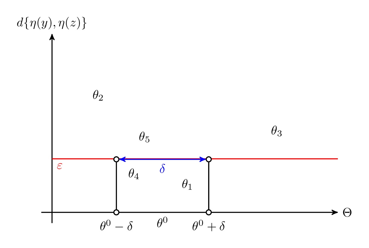
Figure 1: An illustration of ABC output for $N=5$ simulations and given values of $\theta^{0},\delta,\varepsilon,$ and $\mathbf{\eta}(\mathbf{y}).$

The formalization of these statements, along with the precise set of assumptions that a vector of summary statistics, $\mathbf{\eta(y)},$ should satisfy in order for ABC to yield consistent inference, is the content of Theorem 1 and its proof. Subsequent to the presentation of the theorem, we provide a simple example in which the conditions are satisfied, followed by a second example in which they are not. The way in which an increase in the dimension of $\mathbf{\eta(y)}$ can be used to retrieve consistency in the latter case, is then illustrated.

Define the limiting value of the summary statistic based on observed data (respectively, simulated data) as $\mathbf{b(\theta}^{0}\mathbf{)}$ (respectively, $\mathbf{b(\theta}^{i}\mathbf{)}$), and let $\|\cdot\|$ denote the Euclidean norm.

Theorem 1

Let $d\{\cdot,\cdot\}$ be an induced metric on the normed space $(\mathbf{B,}\left\|\cdot\right\|_{\ast})$. Given summary statistics $\mathbf{\eta}(\mathbf{y})$, assume that the following conditions are satisfied:

[S0]

The DGP for $\mathbf{y}$ is uniquely defined at $\mathbf{\theta}^{0}.$

[S1]

$\|\mathbf{\eta}(\mathbf{y})-\mathbf{b}(\mathbf{\theta}^{0})\|=o_{P}(1)$.

[S2]

The map $\mathbf{\theta}^{i}\mapsto\mathbf{b}(\mathbf{\theta}^{i})$ is deterministic, continuous, and satisfies

[S2(1)]

$\sup_{\mathbf{\theta\in\Theta}}\|\mathbf{\eta}(\mathbf{z}(\mathbf{\theta}))-\mathbf{b}(\mathbf{\theta})\|=o_{P}(1)$.

[S2(2)]

$\mathbf{b}(\mathbf{\cdot})$ is one-to-one in $\mathbf{\theta}^{i}$.

If [S0]-[S2] above and [P] are satisfied, then, for any $\delta>0,$ $\text{Pr}_{\varepsilon}(\mathbf{\theta}\notin\aleph_{\delta}(\mathbf{\theta}^{0})|\mathbf{\eta(y))}\overset{P}{\rightarrow}0$ as $T\rightarrow\infty$ and $\varepsilon\rightarrow 0.$

Remark 1

Theorem 1 states that, for ABC based on $\mathbf{\eta}(\cdot)$ to be consistent the limit map $\mathbf{\theta}^{i}\mapsto\mathbf{b}(\mathbf{\theta}^{i})$ must act in the same manner as the “binding function” in indirect inference; see Gouriéroux et al. (1993) and Gouriéroux and Monfort (1996) for a general discussion of binding functions.

Remark 2

Since we are only concerned with Classical Bayesian consistency, Assumption [S0] is implicit and therefore not explicitly required. However, Assumption [S0] is a deep identification condition that may not be satisfied in all circumstances and is therefore maintained to illustrate the scope of the models to which this result will apply. Assumption [S1] is often satisfied under general conditions restricting the dependence in the observed data. Assumption [S2(1)] requires that for all $\xi>0,$

$$\lim_{T\rightarrow\infty}\Pr\left(\sup_{\mathbf{\theta\in\Theta}}\left\|\mathbf{\eta}(\mathbf{z(\theta)})-\mathbf{b}(\mathbf{\theta})\right\|>\xi\right)=0,$$

and is generally referred to as uniform convergence. This stronger notion of convergence is required to ensure that the simulated paths $\mathbf{z(\theta)}$, and the subsequent $\mathbf{\eta}(\mathbf{z(\theta)})$, are well-behaved over $\mathbf{\Theta}$.  General conditions determining satisfaction of [S2(1)] are now well-known and a great many results can be obtained from the empirical process literature; see, for instance, Pollard (1990). In particular, [S2(1)] is likely to be satisfied for many different types of summary statistics so long as the prior density $p(\cdot)$ admits values of $\mathbf{\theta}$ that do not allow the simulated data to display too much persistence.

Remark 3

Theorem 1 requires that the (vector of) summary statistics based on observed data converges, with respect to $d\{\cdot,\cdot\},$ to a fixed quantity and the corresponding vector of statistics based on simulated data $\mathbf{z}^{i}=\mathbf{z(\theta}^{i}\mathbf{)}$ converges (uniformly), with respect to $d\{\cdot,\cdot\},$ to a deterministic function of $\mathbf{\theta}^{i}$. Consistency thus depends not only on the choice of $\mathbf{\eta(y)}$ but also on the precise choice of $d\{\cdot,\cdot\},$ with convergence in one metric not necessarily implying convergence in another. However, restricting $d:\mathbf{B}\times\mathbf{B}\rightarrow\mathbb{R}_{+}$ to be an induced metric  on the normed space $(\mathbf{B,}\left\|\cdot\right\|_{\ast})$ - i.e., for $\mathbf{\eta}_{1}\mathbf{,\eta}_{2}\in\mathbf{B\,}$, requiring that $d\{\mathbf{\eta}_{1}\mathbf{,\eta}_{2}\}=$ $\left\|\mathbf{\eta}_{1}\mathbf{-\eta}_{2}\right\|_{\ast}$ for some norm $\left\|\cdot\right\|_{\ast}$ - relieves the convergence issue since all norms on $\mathbf{B}$ are equivalent to the Euclidean norm $\|\cdot\|$. The requirement that $d\{\cdot,\cdot\}$ be an induced metric is not restrictive as the most common choices of $d\{\cdot,\cdot\}$ satisfy this condition.

Remark 4

Bayesian consistency says that for any $\delta>0$, $p_{\varepsilon}(\mathbf{\theta}|\mathbf{\eta(y)})$ will attribute zero probability, as $T\rightarrow\infty$, to points outside $\aleph_{\delta}(\mathbf{\theta}^{0})$; it does not say anything about how well $p_{\varepsilon}(\mathbf{\theta}|\mathbf{\eta(y)})$ approximates the posterior density $p(\mathbf{\theta|y})$ or even the partial posterior density $p(\mathbf{\theta}|\mathbf{\eta(y)})$. Specifically, the demonstration of Bayesian consistency is distinct from existing theoretical work on ABC that shows $p_{\varepsilon}(\mathbf{\theta}|\mathbf{\eta(y)})$ is consistent for $p(\mathbf{\theta}|\mathbf{\eta(y)})$, as $N\rightarrow\infty$ and $\varepsilon\rightarrow 0,$ for any $\mathbf{\theta\in\Theta}$ and for any fixed T. To prove the latter form of result, researchers have borrowed from the literature on nonparametric density estimation and relied on the idea of mean squared error (MSE) consistency, which requires the bias and variance of $p_{\varepsilon}(\mathbf{\theta}|\mathbf{\eta(y)})-$ $p(\mathbf{\theta}|\mathbf{\eta(y)})$ to approach zero as $N\rightarrow\infty$ and $\varepsilon\rightarrow 0;$ see, for example, Blum (2010) and Biau et al. (2015). In particular, MSE consistency requires a specific rate condition between $N\$and $\varepsilon$ to ensure that the variance of $p_{\varepsilon}(\mathbf{\theta}|\mathbf{\eta(y)})-$ $p(\mathbf{\theta}|\mathbf{\eta(y)})$ shrinks to zero fast enough. As noted in the proof of Theorem 1, Bayesian consistency still requires $N$ to increase as $\varepsilon\rightarrow 0,$ but only to ensure that $p_{\varepsilon}(\mathbf{\theta|\eta(y)})$ exists for small $\varepsilon$, and any $T$. In this way, the particular relationship between $N$ and $\varepsilon$ is independent of the sample size $T$. This lack of any $T$-dependent condition for $\varepsilon$ contrasts with the need for such a condition when deriving results for the asymptotic distribution of ABC point estimators; see, for example, Li and Fearnhead (2015). We elaborate further on this distinction in an on-line supplementary appendix to the paper.

3.2 Success and Failure of Summary Statistic-based ABC

Consistency of ABC based on $\mathbf{\eta}(\cdot)$ hinges on the particular form of $\mathbf{b}(\mathbf{\theta}^{i})$. If $\mathbf{b}(\mathbf{\cdot})$ is one-to-one, i.e., the map $\mathbf{\theta}^{i}\mapsto\mathbf{b}(\mathbf{\theta}^{i})$ satisfies [S2(2)], and the remaining assumptions in Theorem 1 hold, ABC based on $\mathbf{\eta}(\cdot)$ will be consistent. There is generally no guarantee that $\mathbf{b(\cdot)}$ will be one-to-one and satisfaction of this condition depends on both the true structural model and the particular choice of summary statistics. Examples 1 and 2 illustrate a case where [S2(2)] is and is not satisfied, respectively. Example 3 illustrates the impact on identification and, hence, the attainment of consistency, of adding summary statistics to an initial set.

Example 1 (Satisfaction of S2(2) )

Consider the following autoregressive (AR) model of order one:

$$y_{t}=\theta y_{t-1}+\nu_{t},$$

where $\nu_{t}\sim$i.i.d.$N(0,1)$ and $|\theta|<1,\theta\neq 0$. Whilst the likelihood for this model is known in closed form and, hence, exact Bayesian inference is perfectly feasible, for the sake of illustration, consider Algorithm 2 based on the summary statistic $\eta(\mathbf{y})=\frac{1}{T}\sum_{t=2}^{T}y_{t}y_{t-1}$.

Algorithm 2 ABC algorithm: AR(1) example

1:Simulate the AR(1) coefficient $\theta^{i}$ from, for instance, a uniform prior over $(-1,1);$

2:Generate an i.i.d. sequence $\{\nu_{t}\}_{t=1}^{T}$;

3:Produce a simulated series $\{z_{t}^{i}(\theta^{i})\}_{t=1}^{T}$;

4:Accept the value simulated in Step (1) if $d\{\eta(\mathbf{y}),\eta(\mathbf{z}^{i})\}\leq\varepsilon$ for $\varepsilon>0$ and small.

Assume that some true value $\theta^{0}$ has generated the observed sample $\mathbf{y}$. For $p_{\varepsilon}\left(\theta|\eta(\mathbf{y})\right)$ to be degenerate at $\theta^{0}$ it must be that $d\{b(\theta^{0}),b(\theta^{i})\}=0$ has a unique solution $\theta^{i}=\theta^{0}$. By the weak law of large numbers $\eta(\mathbf{y})\overset{P}{\rightarrow}E[y_{t}y_{t-1}]=$ $b(\theta^{0})=\theta^{0}/(1-(\theta^{0})^{2})$ and $\eta(\mathbf{z}^{i})\overset{P}{\rightarrow}E[z_{t}^{i}z_{t-1}^{i}]=$ $b(\theta^{i})=\theta^{i}/(1-(\theta^{i})^{2})$, so $d\{b(\theta^{0}),b(\theta^{i})\}=0$ requires that

$$0=b(\theta^{0})-b(\theta^{i})=(\theta^{i})^{2}\theta^{0}+\theta^{i}(1-(\theta^{0})^{2})-\theta^{0}$$

has unique solution $\theta^{i}=\theta^{0}$. This quadratic equation in $\theta^{i}$ has two solutions: $\theta^{i}=\theta^{0}$ and $\theta^{i}=-1/\theta^{0}$. However, given that $|\theta^{0}|<1,\;\theta^{0}\neq 0$, the second solution is not in the feasible region for $\theta^{i}$ and so ABC based on $\eta(\mathbf{y})=\frac{1}{T}\sum_{t=2}^{T}y_{t}y_{t-1}$ satisfies the conditions of Theorem 1.

Example 2 (Failure of S2(2))

Consider now the moving average (MA) model of order two:

$$y_{t}=e_{t}+\theta_{1}e_{t-1}+\theta_{2}e_{t-2},$$ (3)

where $e_{t}\sim i.i.d.N(0,1)$ and $\theta_{1},\theta_{2}$ satisfy the following invertibility conditions

$$-2<\theta_{1}<2,\;\theta_{1}+\theta_{2}>-1,\theta_{1}-\theta_{2}<1.$$ (4)

Following Marin et al. (2011), we choose as summary statistics the sample autocovariances $\eta_{j}(\mathbf{y})=\frac{1}{T}\sum_{t=1+j}^{T}y_{t}y_{t-j}$, for $j=0,1,2...,K.$ Consider, initially, Algorithm 3, based on $\mathbf{\eta}\left(\mathbf{y}\right)=(\eta_{0}\mathbf{(y)},\eta_{1}\mathbf{(y)})^{\prime}$.

Algorithm 3 ABC algorithm: MA(2) example

1:Simulate the MA(2) coefficients $\mathbf{\theta}^{i\text{ }}$from $p\left(\mathbf{\theta}\right)$ satisfying (4), where $\mathbf{\theta}=(\theta_{1},\theta_{2})^{\prime}$;

2:Generate an i.i.d. sequence $\{e_{t}\}_{t=1}^{T}$;

3:Produce a simulated series $\{z_{t}^{i}\left(\mathbf{\theta}^{i}\right)\}_{t=1}^{T}$;

4:Accept the value generated in Step (1) if $d\{\mathbf{\eta(y)},\mathbf{\eta}(\mathbf{z}^{i})\}\leq\varepsilon$ for $\varepsilon>0$ and small.

Assume that true value $\mathbf{\theta}^{0}=(\theta_{1}^{0},\theta_{2}^{0})^{\prime}$ has generated the observed data $\mathbf{y}$. By the weak law of large numbers $\eta_{0}(\mathbf{y})\overset{P}{\rightarrow}E[y_{t}^{2}]=1+(\theta_{1}^{0})^{2}+(\theta_{2}^{0})^{2}$ and $\eta_{1}(\mathbf{y})\overset{P}{\rightarrow}E[y_{t}y_{t-1}]=\theta_{1}^{0}(1+\theta_{2}^{0})$. In addition, conditional on $\mathbf{\theta}^{i}=(\theta_{1}^{i},\theta_{2}^{i})^{\prime}$ satisfying equation (4), $\eta_{0}(\mathbf{z}^{i})\overset{P}{\rightarrow}1+(\theta_{1}^{i})^{2}+(\theta_{2}^{i})^{2}$ and $\eta_{1}(\mathbf{z}^{i})\overset{P}{\rightarrow}\theta_{1}^{i}(1+\theta_{2}^{i}).$ For $p_{\varepsilon}\left(\mathbf{\theta}|\mathbf{\eta(y)}\right)$ obtained from the above algorithm to be degenerate at $\mathbf{\theta}^{0}$ it must be that for all $\mathbf{\theta}^{i}\mathbf{,\theta}^{0}\mathbf{\in\Theta}$, $0=\mathbf{b}(\mathbf{\theta}^{0})-\mathbf{b}(\mathbf{\theta}^{i})$ has unique solution $\mathbf{\theta}^{i}=\mathbf{\theta}^{0}.$ Clearly,

$$0=\mathbf{b}(\mathbf{\theta}^{0})-\mathbf{b}\left(\mathbf{\theta}^{i}\right)=\begin{pmatrix}1+(\theta_{1}^{0})^{2}+(\theta_{2}^{0})^{2}\\ \theta_{1}^{0}(1+\theta_{2}^{0})\end{pmatrix}-\begin{pmatrix}1+(\theta_{1}^{i})^{2}+(\theta_{2}^{i})^{2}\\ \theta_{1}^{i}(1+\theta_{2}^{i})\end{pmatrix}.$$

As in Marin et al. (2011), take $\theta_{1}^{0}=.6,\theta_{2}^{0}=.2$. Then the question becomes, does there exist $\theta_{1}^{i}\neq.6,\theta_{2}^{i}\neq.2$ such that

$$0=\mathbf{b}(\theta^{0})-\mathbf{b}\left(\theta^{i}\right)=\begin{pmatrix}1+(.6)^{2}+(.2)^{2}\\ .6(1+.2)\end{pmatrix}-\begin{pmatrix}1+(\theta_{1}^{i})^{2}+(\theta_{2}^{i})^{2}\\ \theta_{1}^{i}(1+\theta_{2}^{i})\end{pmatrix}?$$ (5)

Simple numerical calculations reveal that (5) has two solutions: $\theta_{1}^{i}=.6,\theta_{2}^{i}=.2$ and $\theta_{1}^{i}\approx.5453,\theta_{2}^{i}\approx.3204$, where the latter solution remains in the feasible region for $\mathbf{\theta}^{i}=(\theta_{1}^{i},\theta_{2}^{i})^{\prime}.$ Therefore, $\mathbf{b}(\mathbf{\cdot})$ is not one-to-one and the ABC-based posterior will not converge to $\mathbf{\theta}^{0}=(.6,.2)^{\prime}$.

Example 3 (Effect of Additional Statistics)

Consider the same MA(2) model as in Example 2, but now consider the use of the three-dimensional vector of summary statistics:

$$\mathbf{\eta}\left(\mathbf{y}\right)=(\eta_{0}\mathbf{(y)},\eta_{1}\mathbf{(y)},\eta_{2}\mathbf{(y)})^{\prime}.$$

In the language of the generalized method of moments (GMM) literature, the summary statistics of which $\mathbf{\eta}(\mathbf{y})\$is comprised “over-identify” $\mathbf{\theta}^{0}.$ In this case, [S2(2)] will be satisfied if the following equation has a unique solution for all $\mathbf{\theta}^{i},\mathbf{\theta}^{0}$ $\in\Theta$:

$$0=\mathbf{b(\theta}^{0}\mathbf{)-b(\theta}^{i}\mathbf{)}=\left(\begin{array}[]{c}1+(\theta_{1}^{0})^{2}+(\theta_{2}^{0})^{2}\\ \theta_{1}^{0}(1+\theta_{2}^{0})\\ \theta_{2}^{0}\end{array}\right)-\left(\begin{array}[]{c}1+(\theta_{1}^{i})^{2}+(\theta_{2}^{i})^{2}\\ \theta_{1}^{i}(1+\theta_{2}^{i})\\ \theta_{2}^{i}\end{array}\right).$$

The additional (linear) restriction, $0=\theta_{2}^{0}-\theta_{2}^{i},$ ensures that the only value that satisfies $0=\mathbf{b(\theta}^{0}\mathbf{)-b(\theta}^{i}\mathbf{)}$ is now $\mathbf{\theta}^{0}=(\theta_{1}^{0},\theta_{2}^{0})^{\prime}$, and consistency will be achieved as a consequence.

Simply adding summary statistics to the ABC procedure is, however, not guaranteed to yield consistent inference: the chosen summary statistics must be informative about the underlying parameters $\mathbf{\theta}$ governing the statistical properties of the structural model. To illustrate this point, consider again the above example, but with the three-dimensional vector summary statistic:

$$\mathbf{\eta}\left(\mathbf{y}\right)=(\eta_{0}\mathbf{(y),}\eta_{1}\mathbf{(y),}\eta_{3}\mathbf{(y)})^{\prime},$$

where $\eta_{3}(\mathbf{y})=\frac{1}{T}\sum_{t=4}^{T}y_{t}y_{t-3}.$ Given the nature of the structural model, $\eta_{3}(\mathbf{y})\overset{P}{\rightarrow}E[y_{t}y_{t-3}]=0$ and by construction $\eta_{3}(\mathbf{z}^{i})\overset{P}{\rightarrow}E[z_{t}^{i}z_{t-3}^{i}]=0$ for all $\mathbf{\theta}^{i}$. Hence, the summary statistic $\eta_{3}(\mathbf{y})$ yields no new information about $\mathbf{\theta}^{0}$ and does not therefore produce a mapping $\mathbf{\theta}^{i}\longmapsto\mathbf{b(\theta}^{i}\mathbf{)}$ that is one-to-one.

We illustrate the theoretical results in Examples 2 and 3 graphically in Figure 2, denoting the three relevant vectors of summary statistics as:

$$\mathbf{\eta}^{1}\left(\mathbf{y}\right) = (\eta_{0}\mathbf{(y),}\eta_{1}\mathbf{(y)})^{\prime},$$

$$\mathbf{\eta}^{2}\left(\mathbf{y}\right) = (\eta_{0}\mathbf{(y),}\eta_{1}\mathbf{(y),}\eta_{2}\mathbf{(y)})^{\prime},$$

$$\mathbf{\eta}^{3}\left(\mathbf{y}\right) = (\eta_{0}\mathbf{(y),}\eta_{1}\mathbf{(y),}\eta_{3}\mathbf{(y)})^{\prime}.$$

Using the true parameter vector $\mathbf{\theta}^{0}=(\theta_{1}^{0},\theta_{2}^{0})^{\prime}=(0.6,0.2)^{\prime},$ a vector of ‘observed’ data, $\mathbf{y}=(y_{1},y_{2},...,y_{T})^{\prime}$ is generated, for  $T=100,$ $200,$ $500,$ $1,000$ and $5,000$. For each given sample of size $T$, $p(\mathbf{\theta|y})$ is then estimated via the ABC method, using $N=50,000$ simulated draws from uniform priors satisfying (4), and with the tolerance $\varepsilon_{j}$, $j=1,2,3,$ chosen so that only one-percent of the simulated draws are accepted. The top two panels of Figure 2 plot $p_{\varepsilon_{1}}(\theta_{1}\mathbf{|\eta}^{1}\mathbf{(y)})$ and $p_{\varepsilon_{1}}(\theta_{2}\mathbf{|\eta}^{1}\mathbf{(y)})$ respectively, where the notation here indicates the kernel density estimate of the relevant marginal density, conditional on $\mathbf{\eta}^{1}\mathbf{(y)}$, and as defined for the given $\varepsilon_{1}.$ As the sample size increases both estimated marginals become more concentrated, but not around the true values of $0.6$ and $0.2.$ In contrast, the plots in the two middle panels demonstrate the consistency that obtains when conditioning on $\mathbf{\eta}^{2}\mathbf{(y)}$, a result that is not replicated in the two bottom panels, in which the three-dimensional conditioning vector is $\mathbf{\eta}^{3}\left(\mathbf{y}\right).$ 

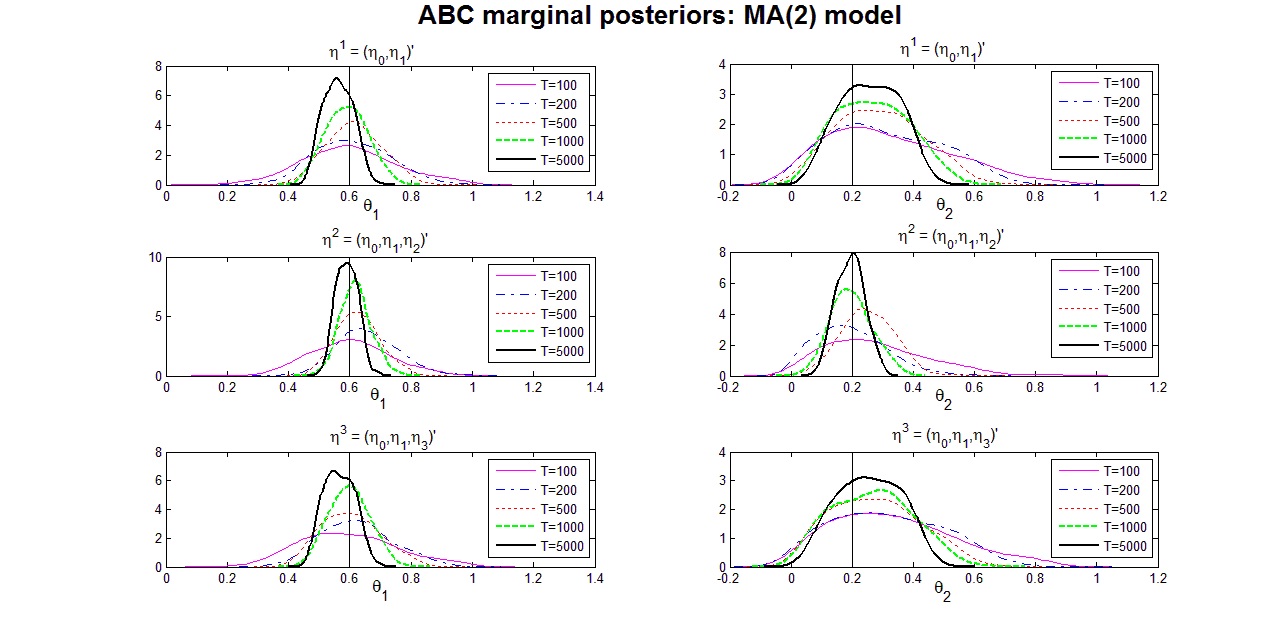
Figure 2: ABC-based estimates of the marginal posterior densities for the parameters of the MA(2) model, $\theta_{1}$ and $\theta_{2}$, with varying sample sizes. Top two panels: summary statistic vector of $\mathbf{\eta}^{1}\left(\mathbf{y}\right)=(\eta_{0}\mathbf{(y),}\eta_{1}\mathbf{(y)})^{\prime}\mathbf{;}$ Middle two panels: summary statistic vector of $\mathbf{\eta}^{2}\left(\mathbf{y}\right)=(\eta_{0}\mathbf{(y),}\eta_{1}\mathbf{(y),}\eta_{2}\mathbf{(y)})^{\prime}\mathbf{;}$ Bottom two panels: summary statistic vector of $\mathbf{\eta}^{3}\left(\mathbf{y}\right)=(\eta_{0}\mathbf{(y),}\eta_{1}\mathbf{(y),}\eta_{3}\mathbf{(y)})^{\prime}\mathbf{.}$ The true parameter values are $\theta_{1}^{0}=0.6$ and $\theta_{2}^{0}=0.2$.

Remark 5

The above example illustrates that adding additional summary statistics to an ABC procedure may or may not aid researchers in obtaining consistent inference. In particular, adding summary statistics will only be helpful if the additional statistics contain information about the parameters that is not accounted for by the summary statistics already used in the analysis. Therefore, arbitrarily adding summary statistics will not necessarily yield valid inference. Moreover, and as was noted in Section 2, given that adding summary statistics hampers our ability to accurately estimate the associated conditional density, adding summary statistics to any initial ABC procedure should be embarked upon with care.

Remark 6

It is also important to note that no link is to be expected between the particular model at hand and the likelihood of Assumption [S2(2)] being satisfied. As the above examples illustrate, it is the combination of the model structure and the choice of summary statistics that determines Bayesian consistency via ABC.

4 Detecting Consistency

4.1 Preliminaries

Beyond understanding the theoretical conditions that must hold in order for a particular set of summary statistics to yield valid inference, and noting that in complex settings verifying the conditions of Theorem 1 will typically not be possible via analytical means, it is useful to have some way of ascertaining numerically whether those conditions actually hold in any given case. To this end, we present a diagnostic tool that can be used to determine if the estimated posterior obtained using a specific set of summary statistics, say $\mathbf{\eta}(\mathbf{y})$, is Bayesian consistent.

The key insight to understanding the diagnostic procedure is that if the true value $\mathbf{\theta}^{0}$ were known, we would only require a local version of the identification condition (Assumption [S2(2)]); i.e., we would only need to check that there existed no $\mathbf{\theta}^{\ast}$, with $\mathbf{\theta}^{\ast}\neq\mathbf{\theta}^{0}$, for which $\mathbf{b}(\mathbf{\theta}^{\ast})=\mathbf{b}(\mathbf{\theta}^{0}).$ However, because $\mathbf{\theta}^{0}$ is unknown, a sufficient condition to ensure that the above holds is that the map $\mathbf{\theta\mapsto b(\theta)}$ is one-to-one; i.e., that $\mathbf{b}(\mathbf{\theta}^{0})-$ $\mathbf{b}(\mathbf{\theta}^{\ast})=\mathbf{0}$ yields the unique solution $\mathbf{\theta}^{\ast}=\mathbf{\theta}^{0}$ for each and every possible value of $\mathbf{\theta}^{0}.$ In this way, detecting Bayesian consistency in ABC reduces to detecting satisfaction of the one-to-one mapping assumption. The diagnostic procedure we propose seeks to verify this condition, and hence the consistency of ABC posterior estimates, in two stages: firstly, as it is applied to the observed data $\mathbf{y}$ (Section 4.2), and secondly, in terms of its repeated application to data sets artificially generated from the assumed true data generating process and across the feasible parameter space (Section 4.3).

The verification procedure exploits the following two facts: 1) under the conditions of Theorem 1, the possible set of solutions for which $d\{\mathbf{\eta}(\mathbf{y}),\mathbf{\eta(z(\theta))}\}=o_{P}(1)$ always includes $\mathbf{\theta}=\mathbf{\theta}^{0}$; 2) if $d\{\mathbf{\eta(y),\eta(z(\theta))}\}=o_{P}(1)$ uniquely at $\mathbf{\theta}=\mathbf{\theta}^{0}$, then an ABC procedure based on an augmented vector of summary statistics, $\mathbf{\gamma(y)}=(\mathbf{\eta}(\mathbf{y})^{\prime},\mathbf{g}(\mathbf{y})^{\prime})^{\prime}$, will yield a posterior that is Bayesian consistent, so long as $\mathbf{g}(\cdot)$ satisfies conditions [S1] and [S2(1)] of Theorem 1. To state these results more formally, assume $\mathbf{\eta}(\mathbf{y})$ (respectively, $\mathbf{g}(\mathbf{y})$) has a well-defined limit $\mathbf{b}_{1}(\mathbf{\theta}^{0})$ (respectively, $\mathbf{b}_{2}(\mathbf{\theta}^{0})$) and denote the limit quantity of $\mathbf{\eta}(\mathbf{z}^{i})$ (respectively, $\mathbf{g}(\mathbf{z}^{i})$) as $\mathbf{b}_{1}(\mathbf{\theta}^{i})$ (respectively, $\mathbf{b}_{2}(\mathbf{\theta}^{i})$).

Corollary 1

Given summary statistics $\mathbf{\gamma(y)}=(\mathbf{\eta}(\mathbf{y})^{\prime},\mathbf{g}(\mathbf{y})^{\prime})^{\prime}$, assume that the following conditions are satisfied:

[C0]

The DGP for $\mathbf{y}$ is uniquely defined at $\mathbf{\theta}^{0}.$

[C1]

For $\mathbf{b}(\mathbf{\theta}^{0})=(\mathbf{b}_{1}(\mathbf{\theta}^{0})^{\prime},\mathbf{b}_{2}(\mathbf{\theta}^{0})^{\prime})^{\prime}$, we have $\|\mathbf{\gamma}(\mathbf{y})-\mathbf{b}(\mathbf{\theta}^{0})\|=o_{P}(1)$.

[C2]

The map $\mathbf{\theta}^{i}\mapsto\mathbf{b}(\mathbf{\theta}^{i})$ is deterministic, continuous, exists for all $\mathbf{\theta}^{i}\in\mathbf{\Theta},$ and satisfies

[C2(1)]

$\sup_{\mathbf{\theta\in\Theta}}\|\mathbf{\gamma}(\mathbf{z}(\mathbf{\theta}))-\mathbf{b}(\mathbf{\theta})\|=o_{P}(1)$,

[C2(2)]

$\mathbf{b}_{1}(\mathbf{\cdot})$ is one-to-one in $\mathbf{\theta}^{i}.$

If [C0]-[C2] and [P] are satisfied, then, for all $\delta>0,$ Pr${}_{\varepsilon}(\mathbf{\theta}\notin\aleph_{\delta}(\mathbf{\theta}^{0})|\mathbf{\gamma(y))}\overset{P}{\rightarrow}0$ as $T\rightarrow\infty$ and $\varepsilon\rightarrow 0$.

4.2 Use of the Observed Data

To understand the implications of Corollary 1, consider the case where we have already obtained $p_{\varepsilon_{1}}(\mathbf{\theta|\eta(y))}$, for some tolerance $\varepsilon_{1},$ with $\mathbf{\eta(y)}$ based on a value of $T$ that is assumed to be large enough for large sample behavior to be in evidence. Now, if we were to run ABC again using the joint summary statistic $\mathbf{\gamma(y)}$, Corollary 1 implies that one of two things will happen: either the posterior $p_{\varepsilon_{2}}(\mathbf{\theta|\gamma(y)),}$ computed for some tolerance $\varepsilon_{2},$ will be located in a very similar position to $p_{\varepsilon_{1}}(\mathbf{\theta|\eta(y))}$, only potentially flatter or with a slightly different shape, a consequence of the increased dimensionality, or the high mass region of $p_{\varepsilon_{2}}(\mathbf{\theta|\gamma(y))}$ will be located in a distinctly different part of the support from that of $p_{\varepsilon_{1}}(\mathbf{\theta|\eta(y))}.$ We refer to this latter event as one of $p_{\varepsilon_{2}}(\mathbf{\theta|\gamma(y))}$ “jumping away” from $p_{\varepsilon_{1}}(\mathbf{\theta|\eta(y))}$ and, according to Corollary 1, see the occurrence of this event as evidence that the initial summary statistics did not yield a posterior that is Bayesian consistent. If, on the other hand, the addition of $\mathbf{g}(\mathbf{y})$ does not cause the mass of $p_{\varepsilon_{2}}(\mathbf{\theta|\gamma(y))}$ to jump in relation to $p_{\varepsilon_{1}}(\mathbf{\theta|\eta(y))}$, then this suggests that the initial choice of summary statistics, $\mathbf{\eta(y),}$ may have yielded valid inference. The use of the word ‘may’ reflects the fact that there is no guarantee possible, via use of the observed data alone, that consistency has been achieved, since there is no guarantee a priori that $d\{\mathbf{\eta(y),\eta(z(\theta))}\}=o_{P}(1)$ has a unique solution $\mathbf{\theta}=\mathbf{\theta}^{0}$. It is this point that is addressed in next subsection.

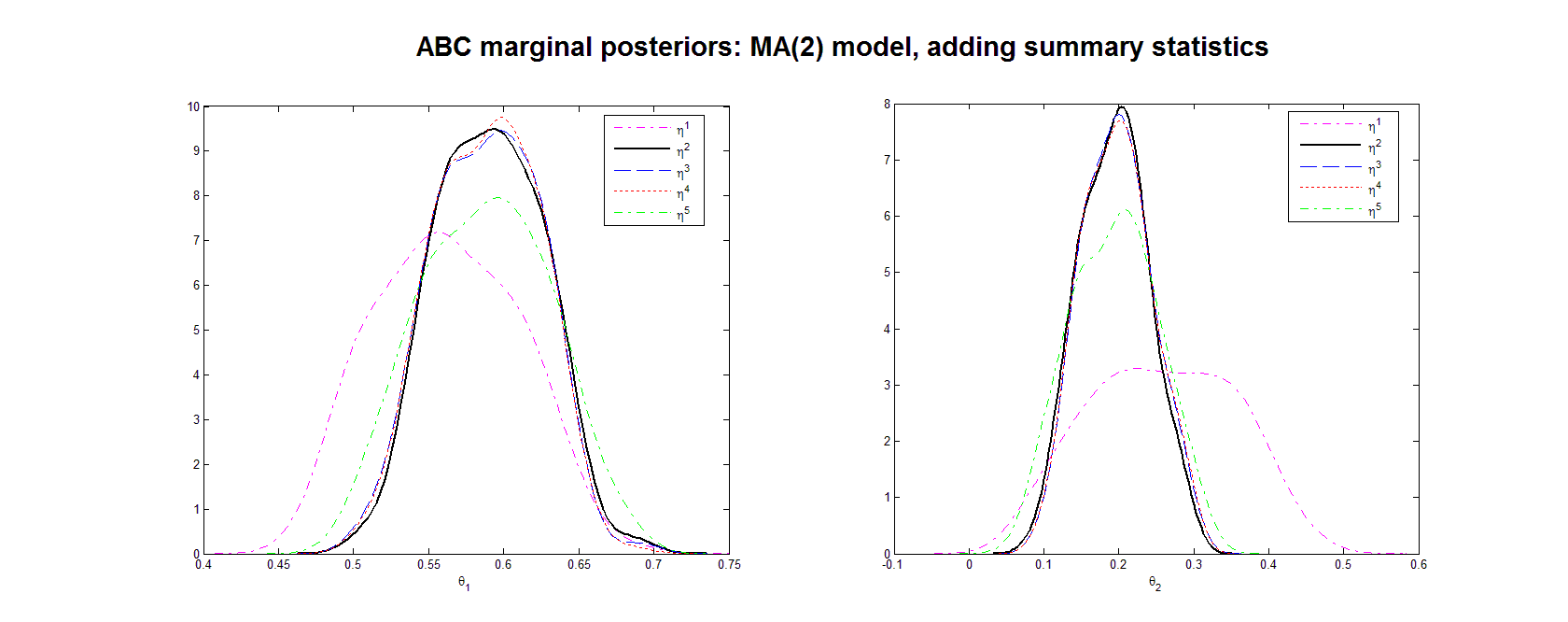
Figure 3: ABC-based estimates of the marginal posterior densities for the parameters of the MA(2) model, $\theta_{1}$ and $\theta_{2}$, with $T=5000$. The key for both panels indicates the summary statistic vector used: $\mathbf{\eta}^{1}\left(\mathbf{y}\right)=(\eta_{0}\mathbf{(y),}\eta_{1}\mathbf{(y)})^{\prime}\mathbf{;}$ $\mathbf{\eta}^{2}\left(\mathbf{y}\right)=(\mathbf{\eta}^{1}(\mathbf{y})^{\prime},\eta_{2}(\mathbf{y}))^{\prime}\mathbf{;}$ $\mathbf{\eta}^{3}(\mathbf{y})=(\mathbf{\eta}^{2}(\mathbf{y})^{\prime},\eta_{3}(\mathbf{y}))^{\prime}\mathbf{;}$ $\mathbf{\eta}^{4}(\mathbf{y})=(\mathbf{\eta}^{3}(\mathbf{y})^{\prime},\frac{1}{T}\sum_{t=1}^{T}y_{t})^{\prime};$ $\mathbf{\eta}^{5}\mathbf{(y)}=(\mathbf{\eta}^{4}(\mathbf{y})^{\prime},\frac{1}{T}\sum_{t=1}^{T}y_{t}^{3})^{\prime}.$ The statistics $\mathbf{\eta}^{2}(\mathbf{y})$ to $\mathbf{\eta}^{5}(\mathbf{y})$ yield Bayesian consistency. The true parameter values are $\theta_{1}^{0}=0.6$ and $\theta_{2}^{0}=0.2$.

Meanwhile, we illustrate this preliminary diagnostic exercise via the MA(2) model, in which case (from Example 3) we have an analytical result that establishes that consistency for the true $\mathbf{\theta}^{0}=(\theta_{1}^{0},\theta_{2}^{0})^{\prime}=(.6,.2)^{\prime}$ is achieved via a particular choice of summary statistics. We adopt five different choices of summary statistics for use in the illustration:

$$\mathbf{\eta}^{1}(\mathbf{y}) = (\eta_{0}(\mathbf{y}),\eta_{1}(\mathbf{y}))^{\prime}$$

$$\mathbf{\eta}^{2}(\mathbf{y}) = (\mathbf{\eta}^{1}(\mathbf{y})^{\prime},\eta_{2}(\mathbf{y}))^{\prime}$$

$$\mathbf{\eta}^{3}(\mathbf{y}) = (\mathbf{\eta}^{2}(\mathbf{y})^{\prime},\eta_{3}(\mathbf{y}))^{\prime}$$

$$\mathbf{\eta}^{4}(\mathbf{y}) = (\mathbf{\eta}^{3}(\mathbf{y})^{\prime},\frac{1}{T}\sum_{t=1}^{T}y_{t})^{\prime}$$

$$\mathbf{\eta}^{5}\mathbf{(y)} = (\mathbf{\eta}^{4}(\mathbf{y})^{\prime},\frac{1}{T}\sum_{t=1}^{T}y_{t}^{3})^{\prime},$$

where $\eta_{j}(\mathbf{y})=\frac{1}{T}\sum_{t=1+j}^{T}y_{t}y_{t-j}\,,$ for $j=0,1,2,3.$ We set the sample size to $T=5,000$, consider $N=50,000$ simulations and set the tolerance $\varepsilon_{j},$ $j=1,...,5$, so that we retain one-percent of the simulated draws for each choice of summary statistics. From our previous theoretical analysis we know that $\mathbf{\eta}^{1}(\mathbf{y})$ will not yield an estimated posterior, $p_{\varepsilon_{1}}(\mathbf{\theta}|\mathbf{\eta}^{1}(\mathbf{y}))$, that is Bayesian consistent, while the remaining sets will yield posteriors that are Bayesian consistent, due to the inclusion of $\eta_{2}\mathbf{(y).}$ Therefore, after adding $\eta_{2}\mathbf{(y)}$ to our initial choice of summary statistics, $\mathbf{\eta}^{1}(\mathbf{y}),$ the estimated posterior $p_{\varepsilon_{2}}(\mathbf{\theta}|\mathbf{\eta}^{2}(\mathbf{y}))$ should be centered around the true values, or thereabouts (given the still finite value of $T$); that is, the main mass of the posterior computed using $\mathbf{\eta}^{2}(\mathbf{y})$ should “jump” away from the main mass of the posterior computed using $\mathbf{\eta}^{1}(\mathbf{y})$. Subsequently, the posteriors based on summary statistics $\mathbf{\eta}^{3}\mathbf{(y)},\mathbf{\eta}^{4}\mathbf{(y)}$ and $\mathbf{\eta}^{5}\mathbf{(y)}$ should not move much, if at all, in relation to $p_{\varepsilon_{2}}(\mathbf{\theta}|\mathbf{\eta}^{2}(\mathbf{y}))$ but may possibly become flatter, and possibly change shape, with each additional summary statistic. Figure 3 illustrates these points exactly. The estimated posterior $p_{\varepsilon_{2}}(\mathbf{\theta}|\mathbf{\eta}^{2}\mathbf{(y)})$ is seen to shift substantially in relation to the estimated posterior $p_{\varepsilon_{1}}(\mathbf{\theta}|\mathbf{\eta}^{1}\mathbf{(y)})$. In turn, adding $\eta_{3}(\mathbf{y})$ and $\frac{1}{T}\sum_{t=1}^{T}y_{t}$ to $\mathbf{\eta}^{2}\mathbf{(y)}$ causes minimal change, and certainly no discernible change in location. The location of the high mass point is preserved by the subsequent addition of $\frac{1}{T}\sum_{t=1}^{T}y_{t}^{3}$; however at this point the dimension of the full statistic $\mathbf{\eta}^{5}\mathbf{(y)}$ appears to cut in, with the accuracy of the kernel density estimation adversely affected.

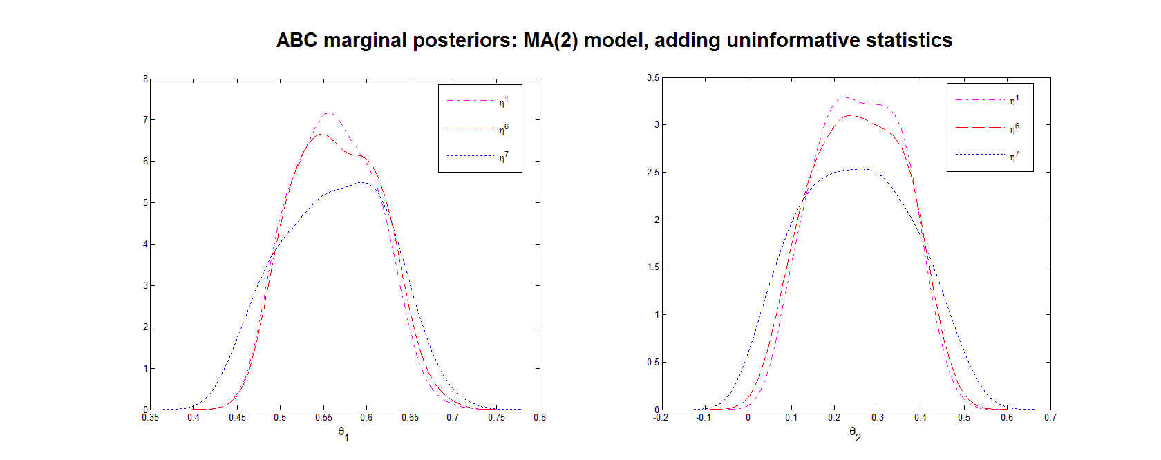
Figure 4: ABC-based estimates of the marginal posterior densities for the parameters of the MA(2) model, $\theta_{1}$ and $\theta_{2}$, with $T=5000$. The key for both panels indicates the summary statistic vector used: $\mathbf{\eta}^{1}\left(\mathbf{y}\right)=(\eta_{0}\mathbf{(y),}\eta_{1}\mathbf{(y)})^{\prime}\mathbf{;}$ $\mathbf{\eta}^{6}\mathbf{(y)}=(\mathbf{\eta}^{1}\mathbf{(y)},\eta_{3}(\mathbf{y}))^{\prime}\mathbf{;}$ $\mathbf{\eta}^{7}\mathbf{(y)}=(\mathbf{\eta}^{6}\mathbf{(y)},\frac{1}{T}\sum_{t=1}^{T}y_{t}^{3})^{\prime}.$ All three summary statistics do not yield Bayesian consistency. The true parameter values are $\theta_{1}^{0}=0.6$ and $\theta_{2}^{0}=0.2$.

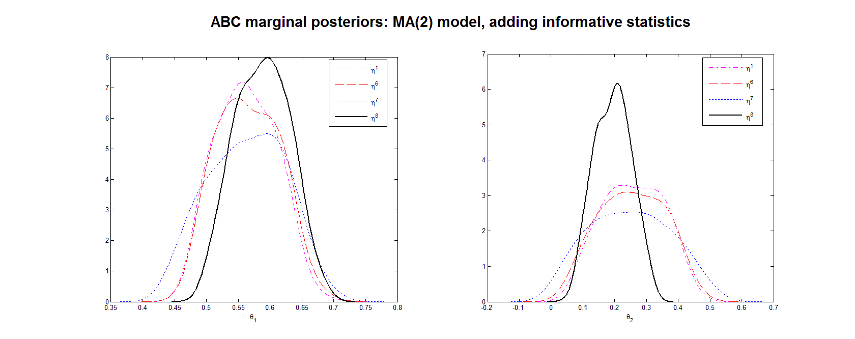
Figure 5: ABC-based estimates of the marginal posterior densities for the parameters of the MA(2) model, $\theta_{1}$ and $\theta_{2}$, with $T=5000$. The key for both panels indicates the summary statistic vector used: $\mathbf{\eta}^{1}\left(\mathbf{y}\right)=(\begin{array}[]{cc}\eta_{0}\mathbf{(y),}&\eta_{1}\mathbf{(y)}\end{array})^{\prime}\mathbf{;}$ $\mathbf{\eta}^{6}\mathbf{(y)}=(\mathbf{\eta}^{1}\mathbf{(y)},\eta_{3}(\mathbf{y}))^{\prime}\mathbf{;}$ $\mathbf{\eta}^{7}\mathbf{(y)}=(\mathbf{\eta}^{6}\mathbf{(y)},\frac{1}{T}\sum_{t=1}^{T}y_{t}^{3})^{\prime};$ $\mathbf{\eta}^{8}\mathbf{(y)}=(\mathbf{\eta}^{7}\mathbf{(y)},\eta_{2}(\mathbf{y}))^{\prime}.$ The first three summary statistics do not yield Bayesian consistency. The fourth is associated with consistency and the marginal posterior estimates are shown to differ markedly from the first three as a consequence. The true parameter values are $\theta_{1}^{0}=0.6$ and $\theta_{2}^{0}=0.2$.

Let us now consider a similar exercise with summary statistics $\mathbf{\eta}^{1}\mathbf{(y)}=(\eta_{0}(\mathbf{y}),\eta_{1}(\mathbf{y}))^{\prime},\mathbf{\eta}^{6}\mathbf{(y)}=(\mathbf{\eta}^{1}\mathbf{(y)},\eta_{3}(\mathbf{y}))^{\prime},\mathbf{\eta}^{7}\mathbf{(y)}=(\mathbf{\eta}^{6}\mathbf{(y)},\frac{1}{T}\sum_{t=1}^{T}y_{t}^{3})^{\prime}$ and $\mathbf{\eta}^{8}\mathbf{(y)}=(\mathbf{\eta}^{7}\mathbf{(y)},\eta_{2}(\mathbf{y}))^{\prime}$, where we deliberately use different notation to distinguish these statistics from those used in the illustration above. In this particular setup the only set of summary statistics that will yield consistent inference is $\mathbf{\eta}^{8}\mathbf{(y)}$, and the aim of the exercise is to illustrate the differential impact of adding non-informative and informative summary statistics to an initial set that does not yield identification. First, consider Figure 4, which plots posteriors based only on $\mathbf{\eta}^{1}\mathbf{(y),\eta}^{6}\mathbf{(y)}$ and $\mathbf{\eta}^{7}\mathbf{(y).}$ Adding $\eta_{3}(\mathbf{y})$ to $\mathbf{\eta}^{1}\mathbf{(y)}$ to produce $\mathbf{\eta}^{6}\mathbf{(y)}$ (which we know does not yield identification) causes the estimated posterior $p_{\varepsilon_{6}}(\mathbf{\theta}|\mathbf{\eta}^{6}(\mathbf{y}))$ to flatten out compared to $p_{\varepsilon_{1}}(\mathbf{\theta}|\mathbf{\eta}^{1}(\mathbf{y}))$, and to shift slightly. Now, adding the statistic $\frac{1}{T}\sum_{t=1}^{T}y_{t}^{3}$ to $\mathbf{\eta}^{6}\mathbf{(y)}$, knowing as we do that this statistic will also not aid in identification, the posterior $p_{\varepsilon_{7}}(\mathbf{\theta}|\mathbf{\eta}^{7}(\mathbf{y}))$ becomes even flatter (reflecting the increased dimension) and continues to shift away from the posterior mode of both previously estimated posteriors, a clear indication that we did not yet have a valid set of summary statistics on the previous rounds.

In Figure 5 we then superimpose on these three plots the estimated marginal posterior based on $\mathbf{\eta}^{8}\mathbf{(y)}$, where we know that the combination of $\mathbf{\eta}^{7}\mathbf{(y)}$ and $\eta_{2}(\mathbf{y})$ (which defines $\mathbf{\eta}^{8}\mathbf{(y)}$) contains sufficient information for the parameters to now be identified. The change in the estimated posterior $p_{\varepsilon_{8}}(\mathbf{\theta}|\mathbf{\eta}^{8}(\mathbf{y}))$, relative to the existing three, is marked, with a clear peak observed around the true values, $\theta_{1}^{0}=0.6$ and $\theta_{2}^{0}=0.2$. Subsequent additions of statistics to this set will, along the lines illustrated in Figure 3, produce posteriors that now remain reasonably fixed at the same modal value and that vary only in terms of dispersion, if at all.

The results of this section are summed up in the following remarks:

Remark 7

Corollary 1 says that if ABC based on summary statistics $\mathbf{\eta}(\mathbf{y})$ yields consistent inference, adding more information, in the form of additional summary statistics, will never invalidate the inference. Typically, adding further statistics can ‘dull’ the inference, in terms of producing a more dispersed posterior, or a posterior with slightly different shape; but it will not shift the mode. Hence, repeated augmentation of an initial choice of statistics, whereby the mode of the estimated posterior eventually ‘settles’ at a particular location, should instill some confidence in the mind of the investigator that consistency may have been achieved.

Remark 8

Whilst the impact of adding non-informative statistics to an initially non-informative set is likely to be problem-specific, we speculate that small and continual changes in both location and dispersion are indicative that a sufficiently informative set of summary statistics has not yet been located. A more substantial shift at some point, followed by a lack of change in the location at least, with the subsequent additions of statistics, is indicative that identification and, hence, consistency, may have been achieved. As flagged above, however, important caveats pertaining to this statement are pursued in the following section.

Remark 9

The above procedure has a similar flavor to the stepwise search algorithm proposed in Joyce and Marjoram (2008). Despite this apparent similarity however, the two procedures differ in terms of their details, as well as having very different objectives. To wit, whilst the approach outlined above is concerned with obtaining a vector of summary statistics that yield consistent inference, that of Joyce and Marjoram is concerned with obtaining a vector of summary statistics that is as informative as possible (or ‘approximately sufficient’ to use their terminology) for any given $T.$

4.3 Use of Repeated Simulation

We have demonstrated how the numerical procedure proposed above can determine with some certainty whether or not $p_{\varepsilon}\mathbf{(\theta|\eta(y))}$ - for some choice of $\mathbf{\eta(y)}$ - is concentrating at $\mathbf{\theta}^{0}$, in the artifical scenario in which $\mathbf{\theta}^{0}$ is known. In practice of course, the true value $\mathbf{\theta}^{0}$ is unknown, and the proposed method is not capable of distinguishing between $p_{\varepsilon}(\mathbf{\theta|\eta(y)})$ concentrating at $\mathbf{\theta}^{0}$ and $p_{\varepsilon}(\mathbf{\theta|\eta(y)})$ concentrating at some other value $\mathbf{\theta}^{\ast}\neq\mathbf{\theta}^{0}$, satisfying $\mathbf{b(\theta}^{\ast}\mathbf{)}=\mathbf{b(\theta}^{0}\mathbf{)}$. However, if the binding function is one-to-one, perverse situations such as the above can be ruled out.

For a fixed (vector) summary statistic, $\mathbf{\eta(y)}$, it turns out that verifying whether or not the binding function is one-to-one is, in principle, possible. To understand how we can verify this condition, first recall that $\mathbf{b(\theta)}$ is simply the limit, as $T\rightarrow\infty$, of the simulated summary statistics$\ \mathbf{\eta(z(\theta))}$, and note that because $\mathbf{z(\theta)}$ is simulated from the structural model, $\mathbf{z(\theta)}$ is no longer restricted to be of the same length as the observed sample $\mathbf{y}$. From these facts, we see that our ability to obtain $\mathbf{b(\theta)}$ is limited only by computational power and time; i.e., we are limited only by our ability to simulate (very) long trajectories for $\mathbf{z(\theta)}$. In addition, the entire map $\mathbf{\theta}\mapsto\mathbf{b(\theta)}$ can be obtained simply by simulating long trajectories of $\mathbf{z(\theta)}$, forming $\mathbf{\eta(z(\theta))}$, and repeating the exercise at every $\mathbf{\theta}\in\mathbf{\Theta}$. Therefore, with enough computing power (and time), it is theoretically possible to verify whether or not $\mathbf{\theta}\mapsto\mathbf{b(\theta)}$ is one-to-one.

While the above logic demonstrates that it is theoretically possible to verify the one-to-one condition, it is not practically possible as this approach (technically) requires simulating an infinite number of infinite series. However, when the data is stationary and the parameter space relatively small, we can approximately check this condition through the following steps:

Algorithm 4 One-to-one verification

1:Use the empirical procedure in Section 4.2 to identify a (vector) summary statistic of interest, hereafter denoted $\mathbf{\eta(\cdot).}$

2:Choose $K^{\ast}$ distinct parameter values with which to simulate data from the structural model, call them $\mathbf{\theta}^{0,1},...,\mathbf{\theta}^{0,K^{\ast}}$. Choose a large integer $T^{\ast}>>T>>0$.

3:Simulate $\widetilde{{\mathbf{z}}}^{k}=(z_{1}(\mathbf{\theta}^{0,k}),...,z_{T^{\ast}}(\mathbf{\theta}^{0,k}))^{\prime}$ and form the series $\left\{\mathbf{\eta}(\widetilde{{\mathbf{z}}}^{k})\right\}_{k=1}^{K^{\ast}}$; $\left\{\mathbf{\eta}(\widetilde{{\mathbf{z}}}^{k})\right\}_{k=1}^{K^{\ast}}$ constitutes a discrete approximation to $\mathbf{\theta}\mapsto\mathbf{b(\theta)}$

4:Determine whether or not $\left\{\mathbf{\eta}(\widetilde{{\mathbf{z}}}^{k})\right\}_{k=1}^{K^{\ast}}$ contains $K^{\ast}$ unique elements.

For $K^{\ast}$ and $T^{\ast}$ large enough, if $\mathbf{\eta}(\cdot)$ satisfies Step (4), and if the estimated $p_{\varepsilon}(\mathbf{\theta}|\mathbf{\eta}(\mathbf{y}))$, as based on the observed data, $\mathbf{y}$, is also collapsing toward some point, one should conclude in favor of consistency. Of course, this process leaves much left unspecified, with the most critical issues being how to span the parameter space, how to selected the set of pre-specified statistics, and the order in which they are to be explored, plus the manner in which degeneracy of the estimated posterior is tested for as $T$ is allowed to increase. However, providing guidelines for and proving the theoretical properties of any such search procedure would require several layers of formalization and the introduction of new terms and concepts that would detract from the current message of the paper. Hence, at this stage we simply emphasize that a completely satisfactory assessment of consistency would appear to require both the use of the observed data and repeated application of data from the assumed process; and suggest that the sort of exercise we are proposing here, albeit informal, is a sensible one to pursue.

5 Criterion Functions based on an Auxiliary Model

5.1 Consistency of Auxiliary Model-based ABC

At a minimum, implementation of ABC requires some means of generating summary statistics $\mathbf{\eta}(\mathbf{y})$ that are “informative” about the unknown parameters of the underlying structural model; whereby “informative” it is generally meant that the summary statistics are a useful way of characterizing the information contained in the observed data. However, the previous sections demonstrate that care must be taken to ensure that the chosen summary statistics yield consistent inference.

An alternative way of obtaining informative summary statistics is through the use of an auxiliary model that depends on parameters $\mathbf{\beta}\in\mathbf{B}\subset\mathbb{R}^{d_{\beta}}$, where $d_{\beta}\geq p$=dim$(\mathbf{\Theta})$, and for which the likelihood function of the auxiliary model, denoted by $L(\mathbf{y};\mathbf{\beta})$, is known in closed form. Given a simple auxiliary likelihood $L(\mathbf{y};\mathbf{\beta})$, a growing literature suggests using summary statistics generated from $L(\mathbf{y};\mathbf{\beta})$; for example, one can choose $\mathbf{\eta}(\mathbf{y})=\mathbf{\widehat{\beta}(y)},$ where $\mathbf{\widehat{\beta}(y)}=\arg\max_{\beta\in\mathbf{B}}L(\mathbf{y};\mathbf{\beta})$, or $\mathbf{\eta}(\mathbf{y})$ equivalent to the vector score of $L(\mathbf{y};\mathbf{\beta})$ evaluated at $\mathbf{\widehat{\beta}(y)}$. However, by its very nature the auxiliary model, and by proxy the summary statistics derived from $L(\mathbf{y};\mathbf{\beta})$, is (are) likely to describe only certain salient features of the underlying structural model. In particular, there is generally no reason to believe that the auxiliary model should “nest” the true structural model in some well-defined sense. Indeed, if it does so then this suggests either that the structural model itself is tractable - hence excluding the need for ABC - or that the nesting model is highly parameterized, thereby inducing a $\mathbf{\eta}(\mathbf{\cdot})$ of high dimension and the associated problems for accuracy.

Given then that a typical auxiliary model is capable of representing only certain salient features of the DGP, there is nothing particularly special about choosing the auxiliary likelihood function to generate summary statistics for use within ABC. Moreover, in many cases a realistic auxiliary model may yield a likelihood function that is itself too complicated for ABC, from a purely computational standpoint, whilst an alternative criterion function, based on the same auxiliary model, may yield computationally simpler summary statistics. For example, alternative criterion functions - other than an auxiliary likelihood - that could be used inside an ABC algorithm include: sums of squared errors, least absolute deviations, and even quadratic functions of sample moments (conditional and unconditional) from an auxiliary model, with the latter used to define an MSM-type of approach, but with moments of the auxiliary rather than the true model defining the selection mechanism.

However, as in the previous section, conditions need to be placed on the relevant criterion function to ensure the resultant ABC procedure yields consistent inference. This is the content of Theorem 2. Begin by defining a sample criterion function based on observed data $\mathbf{y}$ (respectively, simulated data $\mathbf{z}^{i}=\mathbf{z(\theta}^{i}\mathbf{)})$ $Q(\mathbf{y};\mathbf{\beta})$ (respectively, $Q(\mathbf{z}^{i};\mathbf{\beta})$) and define $\mathbf{\widehat{\beta}(y)}$ (respectively, $\mathbf{\widehat{\beta}}(\mathbf{z}^{i})$) as the minimizer of $Q(\mathbf{y};\mathbf{\beta})$ (respectively, $Q(\mathbf{z}^{i};\mathbf{\beta})$). For a particular choice of $Q(\cdot;\mathbf{\beta})$ an ABC algorithm could be based on the summary statistics $\mathbf{\eta(y)=\widehat{\beta}(y)}$, $\mathbf{\eta}(\mathbf{z}^{i})=\mathbf{\widehat{\beta}}(\mathbf{z}^{i})$.

The above intuition yields ABC Algorithm 5 based on generic criterion $Q(.;\mathbf{\beta})$:

Algorithm 5 ABC algorithm: auxiliary criterion function

1:Obtain $\widehat{\mathbf{\beta}}\mathbf{(y)=\arg\min_{\beta\in\mathbf{B}}}Q(\mathbf{y};\mathbf{\beta})$,

2:Simulate $\mathbf{\theta}^{i}$, $i=1,2,...,N$, from $p(\mathbf{\theta})$

3:Simulate $\mathbf{z}^{i}=(z_{1}^{i},z_{2}^{i},...,z_{T}^{i})^{\prime}$, $i=1,2,...,N$, from the likelihood, $p(\mathbf{.|\theta}^{i})$

4:Select $\mathbf{\theta}^{i}$ such that:

$$d\{\mathbf{\eta}(\mathbf{y}),\mathbf{\eta}(\mathbf{z}^{i})\}=d\{\mathbf{\widehat{\beta}(y)},\mathbf{\widehat{\beta}}(\mathbf{z}^{i})\}\leq\varepsilon,$$ (6)

where $d\{\cdot,\cdot\}$ is a distance function (or metric), and the tolerance level $\varepsilon$ is chosen as small as the computing budget allows.

Denote the posterior obtained from the above algorithm as $p_{\varepsilon}^{Q}(\mathbf{\theta}|\mathbf{\eta}(\mathbf{y}))$. The following result gives conditions under which $\text{Pr}_{\varepsilon}^{Q}(\mathbf{\theta\notin\aleph}_{\delta}\mathbf{(\theta}^{0})|\mathbf{\eta}(\mathbf{y}))\overset{P}{\rightarrow}0$ as $T\rightarrow\infty$ and $\varepsilon\rightarrow 0$.

Theorem 2

For an auxiliary model with parameters $\mathbf{\beta}\in\mathbf{B}$, $\mathbf{B}\subset\mathbb{R}^{d_{\beta}}$ compact, assume that the following are satisfied:

[G1]

There exists a deterministic limit criterion function $Q_{\infty}(\mathbf{\theta}^{i};\mathbf{\beta})$ such that

[G1(1)]

$Q_{\infty}(\mathbf{\theta}^{i}\mathbf{;\beta})$ is continuous as a function of $\mathbf{\beta}$, uniformly in $\mathbf{\theta}^{i}$.

[G1(2)]

$\sup_{\beta\in\mathbf{B}}\left|Q(\mathbf{y};\mathbf{\beta})-Q_{\infty}(\mathbf{\theta}^{0}\mathbf{;\beta})\right|=o_{P}(1)$ and $\ \sup_{\mathbf{\theta\in\Theta},\mathbf{\beta}\in\mathbf{B}}\left|Q(\mathbf{z(\theta)};\mathbf{\beta})-Q_{\infty}(\mathbf{\theta;\beta})\right|=o_{P}(1)$

[G2]

$Q_{\infty}(\mathbf{\theta}^{i}\mathbf{;\beta})$ has a unique minimum $\mathbf{b}(\mathbf{\theta}^{i})$ for all $\mathbf{\theta}^{i}\in\mathbf{\Theta}$; i.e., for all $\mathbf{\theta}^{i}\in\mathbf{\Theta}$, $\mathbf{b}(\mathbf{\theta}^{i}):=\arg\min_{\beta\in\mathbf{B}}Q_{\infty}(\mathbf{\theta}^{i}\mathbf{;\beta})$ and $\mathbf{\beta}^{0}:=\mathbf{b}(\mathbf{\theta}^{0}).$

[G3]

$\mathbf{b}\left(\mathbf{\cdot}\right)$ is one-to-one in $\mathbf{\theta}^{i}$; i.e., $\mathbf{\beta}=\mathbf{b}(\mathbf{\theta}^{i})$ has a unique solution for all $\mathbf{\theta}^{i}\in\mathbf{\Theta}$.

If [G1]-[G3] and [P] are satisfied Pr${}_{\varepsilon}^{Q}(\mathbf{\theta}\notin\aleph_{\delta}(\mathbf{\theta}^{0})|\mathbf{\eta(y))}\rightarrow_{p}0$ as $T\rightarrow\infty$ and $\varepsilon\rightarrow 0.$

Remark 10

The above result states that, so long as $Q(\mathbf{.};\mathbf{\beta})$ satisfies standard properties ([G1], [G2]), and if the so-called binding function $\mathbf{b}(\mathbf{\cdot})$ is one-to-one, an ABC algorithm that uses as summary statistics the minimizers of $Q(.;\mathbf{\beta})$ will yield a posterior that is degenerate at $\mathbf{\theta}^{0}$. For a specific objective function, conditions [G1] and [G2] are generally satisfied under more primitive conditions; see, for example, Jennrich (1969) in the setting where $Q(.;\mathbf{\beta})$ is the nonlinear least squares criterion, and Newey and McFadden (1994) in the case where $Q(.;\mathbf{\beta})$ is a minimum distance criterion. While the result of Theorem 2 is intuitive it is nonetheless important as it illustrates that we are not confined to using simple summary statistics of the data or the log-likelihood function $L\left(\mathbf{y};\mathbf{\beta}\right)$ of the auxiliary model within ABC. Instead, any criterion function satisfying [G1]-[G3] can be used to generate valid summary statistics for use in ABC.

Remark 11

An alternative to Algorithm 5 is to replace the summary statistics $\mathbf{\eta(y)}=\widehat{\mathbf{\beta}}(\mathbf{y})$, $\mathbf{\eta}(\mathbf{z}^{i})=\widehat{\mathbf{\beta}}(\mathbf{z}^{i})$ in Step (3) with a distance based on $(\partial/\partial\beta)Q(\mathbf{z}^{i};\mathbf{\widehat{\beta}(y)})$; e.g.,

$$d\left\{\mathbf{\eta(y),\eta(z}^{i}\mathbf{)}\right\}=\sqrt{\left\{(\partial/\partial\mathbf{\beta})Q(\mathbf{z}^{i};\mathbf{\widehat{\beta}(y)})\right\}^{{}^{\prime}}\widehat{\Omega}(\mathbf{y})\left\{(\partial/\partial\mathbf{\beta})Q(\mathbf{z}^{i};\mathbf{\widehat{\beta}(y)})\right\}\text{,}}$$ (7)

for some positive definite weighting matrix $\widehat{\Omega}(\mathbf{y}).$ Such an algorithm would be quite useful in situations where $(\partial/\partial\beta)Q(\mathbf{z}^{i};\mathbf{\widehat{\beta}(y)})$ is known in closed form and would (in all cases) lead to an ABC algorithm that is several orders of magnitude faster than one based on computing $\mathbf{\widehat{\beta}}(\mathbf{z}^{i})$ at every value $\mathbf{\theta}^{i}$. Under conditions similar to those in Theorem 2, a consistency result will hold for the posterior obtained from an ABC algorithm that uses the distance measure in (7). We omit this proof for brevity.

5.2 The Role of the Auxiliary Model

Intimately tied to the idea of choosing a suitable criterion function is the choice of the auxiliary model from which the criterion function is computed. If the chosen auxiliary model is a poor representation of the observed data it is likely that no criterion function, likelihood or otherwise, will produce adequate summary statistics upon which to base our ABC algorithm. In this way using summary statistics from an auxiliary model inside of ABC is not a panacea.

ABC algorithms based on an auxiliary model and with summary statistics derived from a criterion function $Q(.;\mathbf{\beta})$ can fail for precisely the same reason ABC based on arbitrary summary statistics can fail, namely, failure of [G3] (respectively [S2(2)]). Satisfaction of [G3] is affected by both the choice of the auxiliary model and the subsequent criterion function used to obtain $\mathbf{\eta(y)=\mathbf{\widehat{\beta}(}y\mathbf{)}}$. Since the choice of auxiliary model and criterion $Q(.;\mathbf{\beta})$ are user and example specific, attempting to give hard and fast guidelines for how one should choose either is a research topic in its own right. Rather, we simply advocate that validation of [G1]-[G3] should at least be attempted for any specified combination (of model and criterion function) before implementing an ABC algorithm. In the following example we provide support for this statement by illustrating a case in which consistency is not yielded via what seems to be a sensible ABC specification: namely the use of an AR(2) auxiliary model along with an OLS criterion function to produce inference about the true parameters of a MA(2) model.

Example 4

Consider again the MA(2) model from Example 2. Instead of a summary statistic based ABC approach, consider implementing ABC using summary statistics generated via the OLS criterion function for the AR(2) auxiliary model: $y_{t}=\beta_{1}y_{t-1}+\beta_{2}y_{t-2}+\nu_{t}$, with $\nu_{t}\sim(0,1).$ Using

$$Q(\mathbf{y};\mathbf{\beta})=\frac{1}{T}\sum_{t=3}^{T}(y_{t}-\beta_{1}y_{t-1}-\beta_{2}y_{t-2})^{2},$$ (8)

and OLS estimator $\mathbf{\widehat{\beta}(y)}=(\widehat{\beta}_{1}\mathbf{(y)},\widehat{\beta}_{2}\mathbf{(y)})^{\prime}$, the summary statistic $\mathbf{\eta}(\mathbf{y})=(\widehat{\beta}_{1}(\mathbf{y}),\widehat{\beta}_{2}(\mathbf{y}))^{\prime}$, which has a simple closed form, can be used to build a computationally simple ABC algorithm.

Given the particular structure of $Q(\cdot;\mathbf{\beta})$ in (8) and under conditions (4) for $\mathbf{\theta}$, [G1] and [G2] are satisfied. Therefore, all that remains is to verify [G3]. Differentiating the limit criterion $Q_{\infty}(\mathbf{\theta}^{i}\mathbf{;\beta})$ with respect to $\mathbf{\beta}=(\beta_{1},\beta_{2})^{\prime}$ yields the following equations

$$\begin{array}[]{c}E(y_{t-1}(z_{t}^{i}-\beta_{1}z_{t-1}^{i}-\beta_{2}z_{t-2}^{i}))=0,\\ E(y_{t-2}(z_{t}^{i}-\beta_{1}z_{t-1}^{i}-\beta_{2}z_{t-2}^{i}))=0.\end{array}$$ (9)

Defining the autocovariances based on $\mathbf{\theta}^{i}$ as $\gamma_{0}^{i}=(1+(\theta_{1}^{i})^{2}+(\theta_{2}^{i})^{2}),\gamma_{1}^{i}=(\theta_{1}^{i}+\theta_{1}^{i}\theta_{2}^{i})$ and $\gamma_{2}^{i}=\theta_{2}^{i}$, we can re-write (9) as

$$\begin{array}[]{c}\gamma_{1}^{i}-\beta_{1}\gamma_{0}^{i}-\beta_{2}\gamma_{1}^{i}=0,\\ \gamma_{2}^{i}-\beta_{1}\gamma_{1}^{i}-\beta_{2}\gamma_{0}^{i}=0.\end{array}$$ (10)

Solving for $\beta_{1},\beta_{2}$ in (10) yields the following:

$$\beta_{1}(\mathbf{\theta}^{i}):=\left[\gamma_{1}^{i}-\left(\frac{\gamma_{1}^{i}\gamma_{2}^{i}}{\gamma_{0}^{i}}\right)\right]/\left[\gamma_{0}^{i}-\left(\frac{(\gamma_{1}^{i})^{2}}{\gamma_{0}^{i}}\right)\right],\beta_{2}(\mathbf{\theta}^{i}):=\frac{\gamma_{2}^{i}}{\gamma_{0}^{i}}-\frac{\gamma_{1}^{i}}{\gamma_{0}^{i}}\beta_{1}(\mathbf{\theta}^{i}).$$

Interestingly, and as an illustration of the point made in Section 4.1, the binding function $\mathbf{b}(\mathbf{\theta}^{i})=(\beta_{1}(\mathbf{\theta}^{i}),\beta_{2}(\mathbf{\theta}^{i}))^{\prime}$ does not admit a unique solution to $0=\mathbf{\mathbf{b(\mathbf{\theta}^{0})}-b(\theta}^{i}\mathbf{)},$ for all $\mathbf{\theta}^{0},\mathbf{\theta}^{i}$$\in\mathbf{\Theta}$. For instance, simple numerical calculations reveal that if $\mathbf{\theta}^{0}=(\theta_{1}^{0},\theta_{2}^{0})^{\prime}=\left(.6,.2\right)^{\prime}$ the equation $0=\mathbf{\mathbf{b(\mathbf{\theta}^{0})}-b(\theta}^{i}\mathbf{)}$ has a unique solution satisfying the conditions of (4), namely $\mathbf{\theta}^{i}\mathbf{=\theta}^{0}$ (a second solution, $\mathbf{\theta}^{i}=(3,5)^{\prime}$, exists but does not satisfy the parameter restrictions (4)). However, if  $\mathbf{\theta}^{0}=\left(.5,.5\right)^{\prime},$ the equation $0=\mathbf{\mathbf{b(\mathbf{\theta}^{0})}-b(\theta}^{i}\mathbf{)}$ has two solutions satisfying the conditions of (4), $\mathbf{\theta}^{i}\mathbf{=}\left(.5,.5\right)^{\prime}$ and $\mathbf{\theta}^{i}=(1,2)$! Therefore, $\mathbf{b}(\mathbf{\theta}^{i})=(\beta_{1}(\mathbf{\theta}^{i}),\beta_{2}(\mathbf{\theta}^{i}))^{\prime}$ is not a one-to-one function and hence will not yield consistent inference in general.

6 Consistency of ABC in Ordinary Differential Equations Models

In this section we investigate the ability of ABC to yield Bayesian consistent inference for parameters governing a system of ordinary differential equations (ODEs). As will be demonstrated, this particular type of application, which has been given some attention in the ABC literature (see, for example, Toni et al., 2009, Sun et al., 2014, Prangle, 2015), highlights certain important issues related to Bayesian consistency of ABC-based posterior estimates. In particular, by checking the conditions of Theorem 2 in a simple deterministic system, we demonstrate that ABC can yield inconsistent inference in such settings, highlighting the importance of these conditions for verifying the validity of ABC-based inference. While we specifically focus on a simple deterministic system, these findings can easily be generalized to other ODEs.

Specifically, we give our attention to the Lotka-Volterra (LV) model, which describes the interaction between a species $x_{1}$, referred to as the prey species, and a species $x_{2}$, referred to as the predator species. For ${\mathbf{\theta}}=(\theta_{1},\theta_{2})^{\prime}$ unknown, we consider the deterministic LV model defined through the system of ODEs:

$$\frac{dx_{1}}{dt} = \theta_{1}x_{1}-x_{1}x_{2},$$ (11)

$$\frac{dx_{2}}{dt} = \theta_{2}x_{1}x_{2}-x_{2}.$$

For any point $t_{i}$ in the interval $[0,T],$ the vector ${\mathbf{x}}(t_{i})=(x_{1}(t_{i}),x_{2}(t_{i}))^{\prime}$ is the solution to the above ODEs, with initial value $t_{0}.$ Typically, it is assumed that we do not observe ${\mathbf{x}}(t_{i})$; rather, we observe a quantity corresponding to ${\mathbf{x}}(t_{i})$ that is measured with error that is both additive and independent over observational points, see, for example, Beck and Arnold (1977). Following this usual practice then, we specify a measurement equation of the form

$${\mathbf{y}}(t_{i})={\mathbf{x}}(t_{i})+{\mathbf{\nu}}(t_{i}),$$ (12)

where  ${\mathbf{\nu}}(t_{i})\sim i.i.d.(0,\Sigma_{v})$ and $\Sigma_{v}$ is diagonal.

Assume we have an observed sample of size $R_{T}$ from (12), with corresponding design points $t_{1},...,t_{R_{T}},$ fixed or random. Our goal is to estimate the posterior density of ${\mathbf{\theta}}$ using the observed sample $\left\{{\mathbf{y}}(t_{i})\right\}_{i=1}^{R_{T}}\,,$ and prior density $p({\mathbf{\theta}}).$ Toni et al. (2009) propose to estimate these posteriors via ABC using the squared distance between the observed and simulated samples. Specifically, for $\left\{{\mathbf{y}}(t_{i})\right\}_{i=1}^{R_{T}}$ the observed sample and $\left\{{\mathbf{z}}(t_{i};{\mathbf{\theta}})\right\}_{i=1}^{R_{T}}$ the simulated sample, obtained by solving equation (11) at ${\mathbf{\theta}}=(\theta_{1},\theta_{2})^{\prime}$, ABC is based on the distance

$$\rho\left\{\mathbf{y,z(\theta)}\right\}=\frac{1}{R_{T}}\sum_{j=1}^{2}\sum_{i=1}^{R_{T}}(y_{j}(t_{i})-z_{j}(t_{i};\mathbf{\theta})))^{2}.$$ (13)

That is, draws of $\mathbf{\theta}$ are retained according to the proximity of the stochastic quantity $y_{j}(t_{i})$ to the deterministic quantity $z_{j}(t_{i};\mathbf{\theta}).$

It is critical to note, however, that choosing values of $\mathbf{\theta}^{i}$ such that $\rho\left\{\mathbf{y,z(\theta}^{i}\mathbf{)}\right\}\leq\varepsilon$ will not yield an ABC-based posterior that is Bayesian consistent. This can be seen by noting that as $R_{T}\rightarrow\infty,$ even if we select $\mathbf{\theta}^{i}\mathbf{=\theta}^{0}$, and so $x_{j}(t_{i})=z_{j}(t_{i};\mathbf{\theta}^{0})$ for all $t_{i}$ and $j=1,2$, it will be the case that $\lim_{R_{T}\rightarrow\infty}\rho\left\{\mathbf{y,z(\theta}^{0}\mathbf{)}\right\}\overset{P}{\rightarrow}E(\nu_{1}^{2}(t_{i})+\nu_{2}^{2}(t_{i}))>\varepsilon$, for $\varepsilon$ arbitrarily small. Therefore, there exists no value of $\mathbf{\theta}^{i}\in\mathbf{\Theta}$ for which $\rho\left\{\mathbf{y,z(\theta}^{i}\mathbf{)}\right\}\leq\varepsilon$ as $R_{T}\rightarrow\infty$ and $\varepsilon\rightarrow 0,$ and so the ABC-based posterior defined by the distance $\rho\left\{\mathbf{y,z(\theta)}\right\}$ can not be Bayesian consistent.

However, an alternative to the “distance” $\rho\left\{{\mathbf{y,z(\theta)}}\right\}$ in (13) is a metric based on statistics obtained from minimizing an objective function representing the data in equation (12). A common means of obtaining (frequentist) point estimates for parameters defined by ODEs is nonlinear least squares (NLS), whereby the squared distance between the observed and simulated solutions is minimized (see Beck and Anrnold, 1977, for a discussion). This then motivates us to consider the consistency properties of an ABC method that mimics the spirit of NLS. As such, we consider as summary statistics for use in ABC, the parameters that minimize the ordinary least squares (OLS) criterion

$$Q({\mathbf{y;\beta}})=\frac{1}{R_{T}}\sum_{j=1}^{2}\frac{1}{\beta_{2,j}}\sum_{i=1}^{R_{T}}(y_{j}(t_{i})-\beta_{1,j})^{2},$$

with respect to $\mathbf{\beta}=(\mathbf{\beta}_{1}^{\prime},\mathbf{\beta}_{2}^{\prime})^{\prime}$, ${\mathbf{\beta}}_{1}=({\beta}_{1,1},{\beta}_{1,2})^{\prime}$ and ${\mathbf{\beta}}_{2}=({\beta}_{2,1},{\beta}_{2,2})^{\prime},$ which defines $\widehat{\beta}_{1,j}=\frac{1}{R_{T}}\sum_{i=1}^{R_{T}}y_{j}(t_{i})$ as the sample mean and $\widehat{\beta}_{2,j}=\frac{1}{R_{T}}\sum_{i=1}^{R_{T}}(y_{j}(t_{i})-\widehat{\beta}_{1,j})^{2}$ as the sample variance. ABC can then be conducted using $\widehat{{\mathbf{\beta}}}(\mathbf{y})=(\widehat{{\mathbf{\beta}}}_{1}^{\prime}(\mathbf{y}),\widehat{{\mathbf{\beta}}}_{2}^{\prime}(\mathbf{y}))^{\prime}$ and its simulated counterpart $\widehat{{\mathbf{\beta}}}(\mathbf{z}^{i})=(\widehat{{\mathbf{\beta}}}_{1}^{\prime}(\mathbf{z}^{i}),\widehat{{\mathbf{\beta}}}_{2}^{\prime}(\mathbf{z}^{i}))^{\prime}\,,$ with a distance of the form specified in (6) adopted. Further alternatives can be defined by basing ABC on matching $\widehat{{\mathbf{\beta}}}_{1}(\mathbf{y})$ alone (respectively, $\widehat{{\mathbf{\beta}}}_{2}(\mathbf{y})$) with its simulated counterpart $\widehat{{\mathbf{\beta}}}_{1}(\mathbf{z}^{i})$ (respectively, $\widehat{{\mathbf{\beta}}}_{2}(\mathbf{z}^{i})$), with the use of $\widehat{{\mathbf{\beta}}}_{1}(\mathbf{\cdot})$ alone as the matching statistic being closest in spirit to NLS.

Sufficient conditions guaranteeing that ABC will yield consistent inference are given in Theorem 2 and must be verified, for each version of ${\mathbf{\eta(y)}},{\mathbf{\eta(z}^{i}})$ obtained from $Q({\mathbf{\cdot;\beta}}).$ Whilst formal verification of the identification condition in this case is complicated by the fact that ${\mathbf{x}}(t_{i})$ has no closed form, some analytical insights are attainable, by noting the following. Define $\bar{x}_{j}=\lim_{R_{T}\rightarrow\infty}\frac{1}{R_{T}}\sum_{i=1}^{R_{T}}x_{j}(t_{i}),$ $\bar{x}_{j}^{2}=\lim_{R_{T}\rightarrow\infty}\frac{1}{R_{T}}\sum_{i=1}^{R_{T}}x_{j}^{2}(t_{i}),$ and corresponding simulated counterparts $\bar{z}_{j}({\mathbf{\theta}})=\lim_{R_{T}\rightarrow\infty}\frac{1}{R_{T}}\sum_{i=1}^{R_{T}}z_{j}(t_{i};{\mathbf{\theta}}),$ $\bar{z}_{j}^{2}({\mathbf{\theta}})=\lim_{R_{T}\rightarrow\infty}\frac{1}{R_{T}}\sum_{i=1}^{R_{T}}z_{j}^{2}(t_{i};{\mathbf{\theta}}),$ for $j=1,2$. Assuming these quantities exist, it can be shown that

$$\lim_{R_{T}\rightarrow\infty}\widehat{\beta}_{2,j}(\mathbf{y})\xrightarrow{P}\bar{x}_{j}^{2}+\sigma_{j}^{2}-(\bar{x}_{j})^{2},$$

where $\sigma_{j}^{2}$ is the $(j,j)$ element of $\Sigma_{v}$. However, it is also the case that

$$\lim_{R_{T}\rightarrow\infty}\widehat{\beta}_{2,j}({\mathbf{z({\theta})}})\xrightarrow{P}\bar{z}_{j}^{2}({\mathbf{\theta}})-\left(\bar{z}_{j}({\mathbf{\theta}})\right)^{2}.$$

Hence, as $R_{T}\rightarrow\infty$

$$\left\|\widehat{{\mathbf{\beta}}}_{2}(\mathbf{y})-\widehat{{\mathbf{\beta}}}_{2}(\mathbf{z(}{\mathbf{\theta}}^{0}))\right\|\neq o_{P}(1)$$

and so there is no hope that ABC based on ${\mathbf{\eta(y)}}=\widehat{{\mathbf{\beta}}}_{2}(\mathbf{y})$ will yield consistent inference. That is, and reverting to the general notation of the previous section, $Q({\mathbf{y}};{\mathbf{\beta}})$ and $Q({\mathbf{z}}(\mathbf{\theta}^{0});{\mathbf{\beta}})$ do not have corresponding limit $Q_{\infty}(\mathbf{\theta}^{0};{\mathbf{\beta}})$, which violates Assumption [G1] of Theorem 2. This same point pertains to the case in which the augmented statistic $\widehat{{\mathbf{\beta}}}(\mathbf{y})$ is used.

The critical insight from the above illustration, as it pertains to ABC, is that a mismatch between the assumed processes for the observed and simulated data, with the latter failing to replicate the stochastic nature of the former, can create a fundamental disconnect between the matching statistics formed from the two sets of data, so that they will never coincide, no matter the proximity of the drawn parameter vector to the truth. We now contrast this with an alternative approach in which we deliberately draw simulated data according to the measurement equation

$${\mathbf{z}}(t_{i};{\mathbf{\theta}})={\mathbf{w}}(t_{i};{\mathbf{\theta}})+{\mathbf{\tilde{\nu}}}(t_{i}),$$ (14)

where ${\mathbf{w}}(t_{i};{\mathbf{\theta}})$ is the numerical solution of the ODE at parameter value ${\mathbf{\theta}}$ and ${\mathbf{\tilde{\nu}}}(t_{i})$ is a random error drawn from the same distribution as ${\mathbf{\nu}}(t_{i}).$ In this case, it is easy to verify that the simulated statistics $\widehat{{\mathbf{\beta}}}_{2}(\mathbf{z}^{i})\$and $\widehat{{\mathbf{\beta}}}(\mathbf{z}^{i})$ depend on the measurement error variance $\Sigma_{v}$ in the same manner as the observed data, with Assumption [G1] of Theorem 2 no longer violated as a consequence, and so, as $R_{T}\rightarrow\infty$ 

$$\left\|\widehat{{\mathbf{\beta}}}_{2}(\mathbf{y})-\widehat{{\mathbf{\beta}}}_{2}(\mathbf{z(}{\mathbf{\theta}}^{0}))\right\|=o_{P}(1),{\text{ and }}\left\|\widehat{{\mathbf{\beta}}}(\mathbf{y})-\widehat{{\mathbf{\beta}}}(\mathbf{z(}{\mathbf{\theta}}^{0}))\right\|=o_{P}(1).$$

Once again, since no closed form solution exists for the state process, establishing the identification condition analytically, as in the previous examples, is not feasible. However, numerical exploration indicates the existence of consistency for matching statistics $\widehat{{\mathbf{\beta}}}_{1}(y),$ $\widehat{{\mathbf{\beta}}}_{2}(y)$ and $\widehat{{\mathbf{\beta}}}(y)$ when data is simulated according to (14).

It has generally been recognized that consistent inference for point estimates of parameters in ODEs is due to the additive nature of the measurement error, combined with the fact that the measurement error has mean zero, known variance, and is independent of the data, as well as the satisfaction of identification conditions guaranteeing the existence of a unique minimum at $\mathbf{\theta}^{0}$; see, for example, Beck and Arnold (1977). However, when conducting inference for ODEs via ABC, we see that in addition to these conditions (or variants thereof), care must be taken to ensure that data is simulated in such a way that it matches the observed data. It is the price we pay for conducting complete inference using a simulation-based procedure.

7 Discussion

Consistency is one of the most fundamental properties with which to gauge the output of a statistical inference procedure. With our focus on Bayesian consistency, we demonstrate that in the limit (as both $T\rightarrow\infty$ and $\varepsilon\rightarrow 0$) the ABC posterior estimate will be degenerate at the true parameter (vector) if (and only if!) the summary statistics upon which ABC is based are appropriately chosen. Conditions guaranteeing Bayesian consistency of ABC posterior estimates for a wide range of summary statistics, with and without respect to an auxiliary model, with the former defined with respect to an arbitrary criterion function, are developed and several examples featured in the literature are used to illustrate these conditions. The results are less heartening than expected and demonstrate that consistent inference in ABC is in no way guaranteed. In general, we find that ABC will only yield consistent inference when a judicious choice of summary statistics has been employed, subsequently calling into question a large collection of ABC results based on arbitrary summary statistics, as well as those generated from well-specified auxiliary models. In addition, our results highlight the need both to specify a proper distance measure and to ensure an exact match between the process assumed to have generated the observed data and that used to produce simulated samples, in order to have any hope of yielding consistent inference.

To determine if ABC will be Bayesian consistent in practice, we develop a useful and computationally simple diagnostic procedure that can be applied to any given data set and any choice of summary statistics. This procedure constitutes an important first step in determining, in any practical situation, whether ABC will yield consistent inference. Formalization of this diagnostic procedure, as well as work detailing its theoretical properties, is a topic of ongoing research by the authors.

Before closing, we re-emphasize the fact that the results presented herein, while cast within the framework of the ABC accept/reject algorithm, apply to the more sophisticated variants of the ABC method. In particular, the results are applicable to ABC algorithms that generate summary statistics through various simulation-based approximations, as well as algorithms that utilize more efficient methods of post-sampling density estimation. Given this fact, the results discussed herein can be used to form the basic foundation for determining Bayesian consistency for all summary statistic-based ABC algorithms. Further, the key issue that we have emphasized throughout, namely the need to verify the relevant conditions for Bayesian consistency, including the required one-to-one property of the (implied) binding function, is just as pertinent, of course, to related frequentist simulation-based inference methods. In particular, the development of a formal and rigorous method for confirming the one-to-one property of the binding function is as critical to the establishment of the (asymptotic) validity of all other such methods as it is to ABC.

8 Appendix: Proofs

Proof of Theorem 1. The proof is broken into three parts: first, we show that the only value $\mathbf{\theta}^{i}$ that will be selected for all $\varepsilon\geq 0$ as $T\rightarrow\infty$ is $\mathbf{\theta}^{i}=\mathbf{\theta}^{0}$; second, we demonstrate that for any $\varepsilon>0$ there exists some $N(\varepsilon)$ such that if $N>N(\varepsilon)$ the posterior density $p_{\varepsilon}(\mathbf{\theta}|\mathbf{\eta}(\mathbf{y}))$ has a well-defined probability limit; lastly, we use these two pieces to demonstrate that for any $\aleph_{\delta}(\mathbf{\theta}^{0})$ and $\Lambda_{\delta}:=\Theta/\aleph_{\delta}(\mathbf{\theta}^{0})$, the posterior probability $\text{Pr}_{\varepsilon}(\mathbf{\theta}\in\Lambda_{\delta}|\mathbf{\eta}(\mathbf{y}))\xrightarrow{P}0$.

Part 1:

By the triangle inequality

$$d\{\mathbf{\eta}(\mathbf{y}),\mathbf{\eta}(\mathbf{z}^{i})\}\leq d\{\mathbf{\eta}(\mathbf{y}),\mathbf{b}(\mathbf{\theta}^{i})\}+d\{\mathbf{b}(\mathbf{\theta}^{i}),\mathbf{\eta}(\mathbf{z}^{i})\}.$$ (15)

Applying the triangle inequality again to the first term on the right-hand-side of (15) yields

$$d\{\mathbf{\eta}(\mathbf{y}),\mathbf{\eta}(\mathbf{z}^{i})\}\leq d\{\mathbf{b}(\mathbf{\theta}^{0}),\mathbf{b}(\mathbf{\theta}^{i})\}+d\{\mathbf{\eta}(\mathbf{y}),\mathbf{b}(\mathbf{\theta}^{0})\}+d\{\mathbf{b}(\mathbf{\theta}^{i}),\mathbf{\eta}(\mathbf{z}^{i})\}.$$

By [S1], $\mathbf{\eta}(\mathbf{y})\overset{P}{\rightarrow}\mathbf{b}(\mathbf{\theta}^{0})$ and so $d\{\mathbf{\eta}(\mathbf{y}),\mathbf{b}(\mathbf{\theta}^{0})\}=o_{P}(1)$. In addition,

$$d\{\mathbf{\eta}(\mathbf{z}^{i}),\mathbf{b}(\mathbf{\theta}^{i})\}\leq\sup_{\mathbf{\theta\in\Theta}}d\{\mathbf{\eta}(\mathbf{z(\theta)}),\mathbf{b}(\mathbf{\theta})\},$$

and by [S2(1)] $\sup_{\mathbf{\theta\in\Theta}}d\{\mathbf{\eta}(\mathbf{z(\theta)}),\mathbf{b}(\mathbf{\theta})\}=o_{P}(1)$. Combining these facts yields

$$d\{\mathbf{\eta}(\mathbf{y}),\mathbf{\eta}(\mathbf{z}^{i})\}\leq d\{\mathbf{b}(\mathbf{\theta}^{0}),\mathbf{b}(\mathbf{\theta}^{i})\}+o_{P}(1).$$ (16)

For fixed $\varepsilon>0,$ as $T\rightarrow\infty$ a value $\mathbf{\theta}^{i}$ will be selected if

$$d\{\mathbf{b}(\mathbf{\theta}^{0}),\mathbf{b}(\mathbf{\theta}^{i})\}+o_{P}(1)\,\,\leq\varepsilon.$$

By [S2(2)] the only value of $\mathbf{\theta}^{i}\in\mathbf{\Theta}$ for which $\mathbf{b}(\mathbf{\theta}^{i})=\mathbf{b}(\mathbf{\theta}^{0})$ is $\mathbf{\theta}^{i}=\mathbf{\theta}^{0}$. Therefore, as $T\rightarrow\infty$, the only value of $\mathbf{\theta}^{i}$ satisfying $d\{\mathbf{b}(\mathbf{\theta}^{0}),\mathbf{b}(\mathbf{\theta}^{i})\}\leq\varepsilon$ for any $\varepsilon\geq 0$ is $\mathbf{\theta}^{i}=\mathbf{\theta}^{0}$.

Part 2:

Part 1 suggests that for small enough $\varepsilon$ the posterior density $p_{\varepsilon}(\mathbf{\theta}|\mathbf{\eta}(\mathbf{y}))$ will be zero for values $\mathbf{\theta}$ $\in\Lambda_{\delta}$ as $T\rightarrow\infty$. However, because $p_{\varepsilon}(\mathbf{\theta}|\mathbf{\eta}(\mathbf{y}))$ is built from $N$ random draws, for any $\varepsilon>0$ we must ensure that $N$ can be chosen large enough so that $\text{plim}_{T\rightarrow\infty}p_{\varepsilon}(\mathbf{\theta}|\mathbf{\eta}(\mathbf{y}))$ exists for any $\varepsilon>0$.

By compactness of $\mathbf{\Theta}$ and Assumption [P], for any $r>0$ there exists a finite integer $N(r)$ and points $\{\mathbf{\theta}^{i}\}_{i=1}^{N(r)}$, each drawn according to $\mathbf{\theta}^{i}\sim p(\mathbf{\theta})$, such that

$$\mathbf{\Theta}=\bigcup_{i=1}^{N(r)}\aleph_{r}(\mathbf{\theta}^{i})\text{ w.p.1.}$$

By continuity of $\mathbf{b}(\mathbf{\cdot})$, there exists an $r(\varepsilon)>0$ such that, $\|\mathbf{\theta}-\mathbf{\theta}^{0}\|<r(\varepsilon)$ implies $d\{\mathbf{b}(\mathbf{\theta}^{0}),\mathbf{b}(\mathbf{\theta})\}<\varepsilon$ for any $\varepsilon>0$. Combining the two ideas we see that for any $\varepsilon>0$, we can cover $\mathbf{\Theta}$ with $N(r(\varepsilon))$ balls w.p.1. Now, note that by Assumption [P] and the above argument, for any $\varepsilon>0$, we can find a radius $r(\varepsilon)$ such that $\mathbf{\theta}^{0}\in\aleph_{r(\varepsilon)}(\mathbf{\theta}^{i})$ for some $\mathbf{\theta}^{i}$, and $d\{\mathbf{b}(\mathbf{\theta}^{0}),\mathbf{b}(\mathbf{\theta}^{i})\}<\varepsilon\text{{}}\text{ w.p.1}$ as a consequence. In addition, by Assumption [S1], [S2(1)] and Part 1 of the proof,

$$d\{\mathbf{\eta(y)},\mathbf{\eta(z(\theta}^{i}))\}=d\{\mathbf{b(\theta}^{0}),\mathbf{b(\theta}^{i})\}+o_{P}(1)$$

for any $\mathbf{\theta}^{i}\in\mathbf{\Theta}$ and so

$$d\{\mathbf{\eta(y)},\mathbf{\eta(z(\theta}^{i}))\}<\varepsilon+o_{P}(1)$$

for $\mathbf{\theta}^{i}$ such that $\mathbf{\theta}^{0}\in\aleph_{r(\varepsilon)}(\mathbf{\theta}^{i})$. Using this fact, we have that

$$\mathbb{I}_{\varepsilon}[\mathbf{z}(\mathbf{\theta}^{i})]=\mathbb{I}[d\{\mathbf{\eta(y),\eta(z(\theta}^{i}))\}\leq\varepsilon] = \mathbb{I}[d\{\mathbf{b}(\mathbf{\theta}^{0}),\mathbf{b}(\mathbf{\theta}^{i})\}\leq\varepsilon]+o_{P}(1),$$

$$= 1+o_{P}(1).$$

From here we see that for $T$ arbitrarily large and any $\varepsilon>0$, there exists some $N(\varepsilon):=N(r(\varepsilon))$ such that for $N>N(\varepsilon)$

$$p_{\varepsilon}(\mathbf{\theta}|\mathbf{\eta}(\mathbf{y}))=\int_{\mathbf{z}}\frac{p(\mathbf{\theta})p(\mathbf{z}|\mathbf{\theta})\mathbb{I}_{{\varepsilon}}[\mathbf{z}(\mathbf{\theta})]}{\left\{\int_{\mathbf{\Theta}}\int_{\mathbf{z}}p(\mathbf{\theta})p(\mathbf{z}|\mathbf{\theta})\mathbb{I}_{A_{\varepsilon}}[\mathbf{z}(\mathbf{\theta})]d\mathbf{z}d\mathbf{\theta}\right\}}d\mathbf{z}$$ (17)

exists.

Part 3:

We now use Parts 1 and 2 to show that $\text{Pr}_{\varepsilon}(\mathbf{\theta}\in\Lambda_{\delta}|\mathbf{\eta(y)})\xrightarrow{P}0$, where $\Lambda_{\delta}:=\mathbf{\Theta}/\aleph_{\delta}(\mathbf{\theta}^{0})$. By Markov’s inequality

$$\lim_{T\rightarrow\infty}\text{Pr}\bigg{\{}\text{Pr}_{\varepsilon}(\mathbf{\theta}\in\Lambda_{\delta}|\mathbf{\eta}(\mathbf{y}))>\xi\bigg{\}}\leq\lim_{T\rightarrow\infty}\text{E}\bigg{\{}\text{Pr}_{\varepsilon}(\mathbf{\theta}\in\Lambda_{\delta}|\mathbf{\eta}(\mathbf{y}))\bigg{\}}/\xi,$$ (18)

for all $\xi>0$, and the result follows if the left-hand side of (18) is zero. By the definition of $p_{\varepsilon}(\mathbf{\theta}|\mathbf{\eta}(\mathbf{y}))$, $\text{Pr}_{\varepsilon}(\mathbf{\theta}\in A|\mathbf{\eta}(\mathbf{y}))<1$ for any $A\subset\mathbf{\Theta}$, $\varepsilon>0$, and $T\geq 1$. By the bounded convergence theorem

$$\lim_{T\rightarrow\infty}\text{E}\left[\text{Pr}_{\varepsilon}(\mathbf{\theta}\in\Lambda_{\delta}|\mathbf{\eta}(\mathbf{y}))\right]=\text{E}\left[\text{plim}_{T\rightarrow\infty}\text{Pr}_{\varepsilon}(\mathbf{\theta}\in\Lambda_{\delta}|\mathbf{\eta}(\mathbf{y}))\right].$$

By the definition of $p_{\varepsilon}(\mathbf{\theta}|\eta(\mathbf{y}))$ in (17), $\text{Pr}_{\varepsilon}(\mathbf{\theta}\in\Lambda_{\delta}|\mathbf{\eta}(\mathbf{y}))=o_{P}(1)$ only if, for some, $\varepsilon>0$

$$\sup_{\theta\in\Lambda_{\delta}}\mathbb{I}\left[d\{\mathbf{\eta}(\mathbf{y}),\mathbf{\eta}(\mathbf{z}(\mathbf{\theta}))\}\leq\varepsilon\right]=o_{P}(1).$$

For any $\delta>0$, if $\|\mathbf{\theta}-\mathbf{\theta}^{0}\|\geq\delta$, by injectivity of $\mathbf{b}(\cdot)$, it follows that $d\{\mathbf{b}(\mathbf{\theta}),\mathbf{b}(\mathbf{\theta}^{0})\}\geq\varepsilon_{\ast}$ for some $\varepsilon_{\ast}>0$. By compactness of $\Lambda_{\delta}$ and continuity of $\mathbf{b}(\cdot)$, there exists some $\mathbf{\theta}_{\ast}$ (not necessarily unique) such that

$$\mathbf{\theta}_{\ast}=\arg\inf_{\theta\in\Lambda_{\delta}}d\{\mathbf{b}(\mathbf{\theta}^{0}),\mathbf{b}(\mathbf{\theta})\},$$ (19)

and, by injectivity of $\mathbf{b}(\cdot),$ for some $\varepsilon_{\ast}>0$

$$d\{\mathbf{b}(\mathbf{\theta}^{0}),\mathbf{b}(\mathbf{\theta}_{\ast})\}\geq\varepsilon_{\ast}>0.$$ (20)

Moreover, by Assumptions [S1], [S2(1)], and equation (16) in Part 1,

$$\sup_{\theta\in\Lambda_{\delta}}|\mathbb{I}_{\varepsilon}[\mathbf{z}(\mathbf{\theta})]-\mathbb{I}_{\varepsilon}[\mathbf{b}(\mathbf{\theta})]|=\sup_{\theta\in\Lambda_{\delta}}|\mathbb{I}[d\{\mathbf{\eta}(\mathbf{y}),\mathbf{\eta}(\mathbf{z}(\mathbf{\theta}))\}\leq\varepsilon]-\mathbb{I}[d\{\mathbf{b}(\mathbf{\theta}^{0}),\mathbf{b}(\mathbf{\theta})\}\leq\varepsilon]|=o_{P}(1).$$ (21)

From equation (21) it follows that

$$\mathbb{I}[d\{\mathbf{\eta}(\mathbf{y}),\mathbf{\eta}(\mathbf{z}(\mathbf{\theta_{\ast}}))\}\leq\varepsilon]=\mathbb{I}[d\{\mathbf{b}(\mathbf{\theta}^{0}),\mathbf{b}(\mathbf{\theta_{\ast}})\}\leq\varepsilon]+o_{P}(1).$$

By the definition of $\mathbf{\theta}_{\ast}$ in (19) and equation (20), for any $\varepsilon^{\ast}<\varepsilon_{\ast}$,

$$\mathbb{I}[d\{\mathbf{b}(\mathbf{\theta}^{0}),\mathbf{b}(\mathbf{\theta_{\ast}})\}\leq\varepsilon^{\ast}]=0.$$

We can then conclude that

$$\mathbb{I}[d\{\mathbf{\eta}(\mathbf{y}),\mathbf{\eta}(\mathbf{z}(\mathbf{\theta}_{\ast})\}\leq\varepsilon^{\ast}]=o_{P}(1).$$

Moreover, from equation (19)

$$\inf_{\theta\in\Lambda_{\delta}}d\{\mathbf{b}(\mathbf{\theta}^{0}),\mathbf{b}(\mathbf{\theta})\}=d\{\mathbf{b}(\mathbf{\theta}^{0}),\mathbf{b}(\mathbf{\theta_{\ast}})\}\geq\varepsilon_{\ast}>\varepsilon^{\ast},$$ (22)

and so it follows from (21) and equation (22)

$$\sup_{\theta\in\Lambda_{\delta}}\mathbb{I}[d\{\mathbf{\eta}(\mathbf{y}),\mathbf{\eta}(\mathbf{z}(\mathbf{\theta}))\}\leq\varepsilon^{\ast}]=o_{P}(1).$$

Therefore, for $\varepsilon\leq\varepsilon^{\ast}$ and a corresponding $N>N(\varepsilon)$ number of simulated draws, which exists by Part 2, $\text{Pr}_{\varepsilon}(\mathbf{\theta}\in\Lambda_{\delta}|\mathbf{\eta}(\mathbf{y}))=o_{P}(1)$ and the result follows.    

Proof of Corollary 1. We have two cases to consider: one, the vector $\mathbf{b}(\mathbf{\theta}^{i})$ is one-to-one in $\mathbf{\theta}^{i}$ and two, only the sub-vector $\mathbf{b}_{1}(\mathbf{\theta}^{i})$ is one-to-one in $\mathbf{\theta}^{i}$. Clearly, if the first case obtains then the result follows from Theorem 1 and so we can focus on the latter case.

For the second case then, by the triangle inequality

$$d\{\mathbf{\gamma}(\mathbf{y}),\mathbf{\gamma}(\mathbf{z^{i}})\}\leq d\{\mathbf{\gamma}(\mathbf{y}),\mathbf{b}(\mathbf{\theta}^{i})\}+d\{\mathbf{b}(\mathbf{\theta}^{i}),\mathbf{\gamma}(\mathbf{z}^{i})\}.$$ (23)

Using the same arguments as in Theorem 1, equation (23) can be restated as

$$d\{\mathbf{\gamma}(\mathbf{y}),\mathbf{\gamma}(\mathbf{z^{i}})\}\leq d\{\mathbf{b}(\mathbf{\theta}^{0}),\mathbf{b}(\mathbf{\theta}^{i})\}+o_{P}(1).$$

By assumption $d\{\cdot,\cdot\}$ is an induced metric, and so for vectors $x$ and $z$ (of the same dimension) $d\{x,z\}=0$ if and only if $x=z.$ Using this fact we see that

$$d\{\mathbf{b}(\mathbf{\theta}^{0}),\mathbf{b}(\mathbf{\theta})\}=0\iff\left(\begin{array}[]{c}\mathbf{b}_{1}\mathbf{(\theta}^{0}\mathbf{)}\\ \mathbf{b}_{2}\mathbf{(\theta}^{0}\mathbf{)}\end{array}\right)=\left(\begin{array}[]{c}\mathbf{b}_{1}\mathbf{(\theta)}\\ \mathbf{b}_{2}\mathbf{(\theta)}\end{array}\right).$$

The key observation is that the set $S_{\mathbf{\theta}}:=\left\{\theta\in\Theta:\|\mathbf{b}_{2}(\mathbf{\theta}^{0})-\mathbf{b}_{2}(\mathbf{\theta})\|=0\right\}$ always includes the point $\mathbf{\theta=\theta}^{0}$, but can include other points since $\mathbf{b}_{2}\mathbf{(\cdot)}$ need not be one-to-one. However, by [C2(2)], we know that $\mathbf{b}_{1}(\mathbf{\cdot})$ is one-to-one and so the only value of $\mathbf{\theta}$ for which

$$\left(\begin{array}[]{c}\mathbf{b}_{1}\mathbf{(\theta}^{0}\mathbf{)}\\ \mathbf{b}_{2}\mathbf{(\theta}^{0}\mathbf{)}\end{array}\right)-\left(\begin{array}[]{c}\mathbf{b}_{1}\mathbf{(\theta)}\\ \mathbf{b}_{2}\mathbf{(\theta)}\end{array}\right)=\left(\begin{array}[]{c}0\\ 0\end{array}\right),$$

is $\mathbf{\theta=\theta}^{0}.$ The result then follows by the same arguments as in Theorem 1.    

Proof of Theorem 2. By the triangle inequality

$$d\{\mathbf{\widehat{\beta}}(\mathbf{y}),\mathbf{\widehat{\beta}}(\mathbf{z}^{i})\}\leq d\{\mathbf{\widehat{\beta}}(\mathbf{y}),\mathbf{b}(\mathbf{\theta}^{i})\}+d\{\mathbf{b}(\mathbf{\theta}^{i}),\mathbf{\widehat{\beta}}(\mathbf{z}^{i})\}.$$ (24)

Before proceeding further we must show that, under the maintained assumptions,

$$\sup_{\mathbf{\theta\in\Theta}}\left\|\mathbf{\widehat{\beta}}(\mathbf{z}(\mathbf{\theta}))-\mathbf{b}(\mathbf{\theta})\right\|=o_{P}(1).$$ (25)

Define the following terms:

$$\widetilde{Q}(\mathbf{\theta,\beta}) = Q(\mathbf{z}(\mathbf{\theta}),\mathbf{\beta})-Q_{\infty}(\mathbf{\theta},\mathbf{b}(\mathbf{\theta})),$$

$$\widetilde{Q}_{\infty}(\mathbf{\theta,\beta}) = Q_{\infty}(\mathbf{\theta,\beta})-Q_{\infty}(\mathbf{\theta},\mathbf{b}(\mathbf{\theta})).$$

Note that, by [G1(1)], for all $\delta>0$, if $\sup_{\mathbf{\theta\in\Theta}}\|\widehat{\mathbf{\beta}}(\mathbf{z}(\mathbf{\theta)})-\mathbf{b}(\mathbf{\theta})\|>\delta,$ there exists $\epsilon(\delta)>0$, such that

$$\sup_{\mathbf{\theta\in\Theta}}\|Q_{\infty}(\mathbf{\theta},\widehat{\mathbf{\beta}}(\mathbf{z}(\mathbf{\theta)}))-Q_{\infty}(\mathbf{\theta},\mathbf{b}(\mathbf{\theta}))\|=\sup_{\mathbf{\theta\in\Theta}}\|\widetilde{Q}_{\infty}(\mathbf{\theta},\widehat{\mathbf{\beta}}(\mathbf{z}(\mathbf{\theta)}))\|>\epsilon(\delta).$$

From here, note that

$$\text{Pr}\left(\sup_{\mathbf{\theta\in\Theta}}\|\widehat{\mathbf{\beta}}(\mathbf{z}(\mathbf{\theta)})-\mathbf{b}(\mathbf{\theta})\|>\delta\right)\leq\text{Pr}\left(\sup_{\mathbf{\theta\in\Theta}}\|\widetilde{Q}_{\infty}(\mathbf{\theta},\widehat{\mathbf{\beta}}(\mathbf{z}(\mathbf{\theta)}))\|>\epsilon(\delta)\right).$$

The result in (25) then follows if $\sup_{\mathbf{\theta\in\Theta}}\|\widetilde{Q}_{\infty}(\mathbf{\theta},\widehat{\mathbf{\beta}}(\mathbf{z}(\mathbf{\theta)}))\|=o_{P}(1)$.

Uniformly in $\mathbf{\theta}$,

$$\|\widetilde{Q}_{\infty}(\mathbf{\theta},\widehat{\mathbf{\beta}}(\mathbf{z}(\mathbf{\theta)})))\| \leq \|\widetilde{Q}_{\infty}(\mathbf{\theta},\widehat{\mathbf{\beta}}(\mathbf{z}(\mathbf{\theta)}))-\widetilde{Q}(\mathbf{\theta},\widehat{\mathbf{\beta}}(\mathbf{z}(\mathbf{\theta)}))\|+\|\widetilde{Q}(\mathbf{\theta},\widehat{\mathbf{\beta}}(\mathbf{z}(\mathbf{\theta)}))\|$$ (26)

$$= \|Q_{\infty}(\mathbf{\theta,}\widehat{\mathbf{\beta}}(\mathbf{z}(\mathbf{\theta)}))-Q(\mathbf{z}(\mathbf{\theta),}\widehat{\mathbf{\beta}}(\mathbf{z}(\mathbf{\theta)}))\|+\|\widetilde{Q}(\mathbf{\theta},\widehat{\mathbf{\beta}}(\mathbf{z}(\mathbf{\theta)}))\|$$

$$\leq \sup_{\mathbf{\beta}\in\mathbf{B}}\|Q_{\infty}(\mathbf{\theta},\mathbf{\beta})-Q(\mathbf{z}(\mathbf{\theta}),\mathbf{\beta})\|+\|\widetilde{Q}(\mathbf{\theta},\widehat{\mathbf{\beta}}(\mathbf{z}(\mathbf{\theta)}))\|$$

$$\leq o_{P}(1)+\|\widetilde{Q}(\mathbf{\theta},\widehat{\mathbf{\beta}}(\mathbf{z}(\mathbf{\theta)}))\|.$$

The first inequality follows from the triangle inequality, the second from the definition of $\widetilde{Q}_{\infty}(\mathbf{\theta},\mathbf{\beta})$ and $\widetilde{Q}(\mathbf{\theta},\mathbf{\beta})$, the third from the definition of $\sup,$ and the last from Assumption [G1(2)].

From (26), the result follows if

$$\sup_{\mathbf{\theta}\in\mathbf{\Theta}}\|\widetilde{Q}(\mathbf{\theta},\widehat{\mathbf{\beta}}(\mathbf{z}(\mathbf{\theta})))\|=o_{P}(1).$$

By the definition of $\widehat{\mathbf{\beta}}(\mathbf{z}(\mathbf{\theta}))$, uniformly in $\mathbf{\theta}$,  

$$\|\widetilde{Q}(\mathbf{\theta},\widehat{\mathbf{\beta}}(\mathbf{z}(\mathbf{\theta)}))\| \leq \inf_{\mathbf{\beta}\in\mathbf{B}}\|\widetilde{Q}(\mathbf{\theta},\mathbf{\beta})\|+o_{P}(1)$$ (27)

$$\leq \inf_{\mathbf{\beta}\in\mathbf{B}}\|\widetilde{Q}(\mathbf{\theta},\mathbf{\beta})-\widetilde{Q}_{\infty}(\mathbf{\theta},\mathbf{\beta})\|+\inf_{\mathbf{\beta}\in\mathbf{B}}\|\widetilde{Q}_{\infty}(\mathbf{\theta},\mathbf{\beta})\|+o_{P}(1)$$

$$\leq \sup_{\mathbf{\beta}\in\mathbf{B}}\|Q(\mathbf{z}(\mathbf{\theta}),\mathbf{\beta})-Q_{\infty}(\mathbf{\theta},\mathbf{\beta})\|+0+o_{P}(1)$$

$$\leq o_{P}(1),$$

with the last inequality following from [G1(2)]. Combining equations (26) and (27) yields $\sup_{\mathbf{\theta\in\Theta}}\left\|\mathbf{\widehat{\beta}}(\mathbf{z}(\mathbf{\theta}))-\mathbf{b}(\mathbf{\theta})\right\|=o_{P}(1),$ and we can conclude

$$d\{\widehat{\mathbf{\beta}}(\mathbf{z}^{i}),\mathbf{b}(\mathbf{\theta}^{i})\}\leq\sup_{\mathbf{\theta}\in\mathbf{\Theta}}d\{\mathbf{\widehat{\beta}}(\mathbf{z}(\mathbf{\theta})),\mathbf{b}(\mathbf{\theta})\}=o_{P}(1).$$ (28)

Applying equation (28) to equation (24) we have

$$d\{\mathbf{\widehat{\beta}}(\mathbf{y}),\mathbf{\widehat{\beta}}(\mathbf{z}^{i})\}\leq d\{\mathbf{\widehat{\beta}}(\mathbf{y}),\mathbf{b}(\mathbf{\theta}^{i})\}+o_{P}(1).$$ (29)

Applying the triangle inequality to $d\{\mathbf{\widehat{\beta}}(\mathbf{y}),\mathbf{b}(\mathbf{\theta}^{i})\}$ yields

$$d\{\mathbf{\widehat{\beta}}(\mathbf{y}),\mathbf{b}(\mathbf{\theta}^{i})\}\leq d\{\mathbf{\widehat{\beta}}(\mathbf{y}),\mathbf{b}(\mathbf{\theta}^{0})\}+d\{\mathbf{b}(\mathbf{\theta}^{0}),\mathbf{b}(\mathbf{\theta}^{i})\}+o_{P}(1),$$

By [G1] and [G2], $\left\|\mathbf{\widehat{\beta}}(\mathbf{y})-\mathbf{b}(\mathbf{\theta}^{0})\right\|=o_{P}(1),$ and so

$$d\{\mathbf{\widehat{\beta}}(\mathbf{y}),\mathbf{b}(\mathbf{\theta}^{i})\}\leq d\{\mathbf{b}(\mathbf{\theta}^{0}),\mathbf{b}(\mathbf{\theta}^{i})\}+o_{P}(1).$$ (30)

From (29) and (30) we thus have

$$d\{\mathbf{\widehat{\beta}}(\mathbf{y}),\mathbf{\widehat{\beta}}(\mathbf{z}^{i})\}\leq d\{\mathbf{b}(\mathbf{\theta}^{0}),\mathbf{b}(\mathbf{\theta}^{i})\}+o_{P}(1).$$

For fixed ${\varepsilon}\geq 0$, as $T\rightarrow\infty$ a value $\mathbf{\theta}^{i}$ will be selected if and only if

$$d\{\mathbf{b}(\mathbf{\theta}^{0}),\mathbf{b}(\mathbf{\theta}^{i})\}+o_{P}(1)\,\,\leq\varepsilon.$$

By [G3] the only value of $\mathbf{\theta}^{i}\in\mathbf{\Theta}$ for which $\mathbf{b}\left(\mathbf{\theta}^{i}\right)=\mathbf{b}\left(\mathbf{\theta}^{0}\right)$ is $\mathbf{\theta}^{i}\mathbf{=\theta}^{0}$. Therefore, the only value of $\mathbf{\theta}^{i}$ satisfying $d\{\mathbf{b}(\mathbf{\theta}^{0}),\mathbf{b}(\mathbf{\theta}^{i})\}\leq\varepsilon$ as $\varepsilon\rightarrow 0$ is $\mathbf{\theta}^{i}\mathbf{=\theta}^{0}$. The result follows using similar arguments to those of Theorem 1.

References

- [1] Beaumont, M.A., Cornuet, J-M., Marin, J-M. and Robert, C.P. 2009. Adaptive Approximate Bayesian Computation, Biometrika, 96, 983–990.
- [2] Beaumont, M.A., Zhang, W. and Balding, D.J. 2002. Approximate Bayesian Computation in Population Genetics, Genetics, 162, 2025–2035.
- [3] Beck, J.V. and Arnold, K.J. 1977. Parameter Estimation in Engineering and Science, John Wiley & Sons.
- [4] Biau, G., Cérou, F. and Guyader, A. 2015. New insights into Approximate Bayesian Computation. Ann. Inst. H. Poincaré Probab. Statist., 51, 376–403.
- [5] Blackwell, D. and Dubins, L. 1962. Merging of Opinions with Increasing Information, Ann. Statist., 33, 882–886.
- [6] Blum, M.G.B. 2010. Approximate Bayesian Computation: a Nonparametric Perspective, Journal of the American Statistical Association, 105, 1178-1187.
- [7] Blum, M.G.B. and François, O. 2010. Non-linear Regression Models for Approximate Bayesian Computation, Statistics and Computing, 20, 63–73.
- [8] Blum, M.G.B., Nunes, M.A., Prangle, D. and Sisson, S.A. 2013. A Comparative Review of Dimension Reduction Methods in Approximate Bayesian Computation, Statistical Science, 28, 189–208.
- [9] Creel, M. and Kristensen, D. 2015. ABC of SV: Limited Information Likelihood Inference in Stochastic Volatility Jump-Diffusion Models, Journal of Empirical Finance, 31, 85-108.
- [10] Diaconis, P. and Freedman, D. 1986. On the Consistency of Bayes Estimates, Ann. Statist., Vol 14, no. 1, 1–26.
- [11] Drovandi, C.C., Pettitt, A.N. and Faddy, M.J. 2011. Approximate Bayesian Computation Using Indirect Inference, J. Royal Statistical Soc. Series C, 60 1 –21.
- [12] Drovandi, C. C., Pettitt, A. N. and Lee, A. 2015. Bayesian Indirect Inference using a Parametric Auxiliary Model. Statistical Science, 30, 72–95.
- [13] Duffie, D. and Singleton, K.J. 1993. Simulated Moments Estimation of Markov Models of Asset Prices, Econometrica, 64, 929–952.
- [14] Fearnhead, P. and Prangle, D. 2012. Constructing Summary Statistics for Approximate Bayesian Computation: Semi-automatic Approximate Bayesian Computation. J. Royal Statistical Soc. Series B, 74, 419–474.
- [15] Gallant, A.R. and Tauchen, G. 1996. Which Moments to Match, Econometric Theory, 12, 657–681.
- [16] Ghosal, S., Ghosh, J.K. and Samanta, T. 1995. On Convergence of Posterior Distributions. Ann. Statist., 23, 2145–2152.
- [17] Gleim, A. and Pigorsch, C. 2013. Approximate Bayesian Computation with Indirect Summary Statistics. Draft paper: http://ect-pigorsch.mee.uni-bonn.de/data/research/papers/.
- [18] Gouriéroux, C. and Monfort, A. 1996. Simulation-based Econometric Methods, OUP.
- [19] Gouriéroux, C., Monfort, A. and Renault, E. 1993. Indirect Inference, Journal of Applied Econometrics, 85, S85–S118.
- [20] Heggland, K. and Frigessi, A. 2004. Estimating Functions in Indirect Inference, J. Royal Statistical Soc. Series B, 66, 447–462.
- [21] Ibragimov, I. A. and Has’minskii, R. Z. 1981. Statistical Estimation: Asymptotic Theory. Springer, New York.
- [22] Jennrich, R. I. 1969. Asymptotic Properties of Non-Linear Least Squares Estimators. Ann. Math. Statist., 40, 633–643.
- [23] Joyce, P. and Marjoram, P. 2008. Approximately Sufficient Statistics and Bayesian Computation. Statistical applications in genetics and molecular biology, 7, 1–16.
- [24] Le Cam. 1953. On Some Asymptotic Properties of Maximum Likelihood Estimates and Related Bayes Estimates. University of California Publications in Statistics, 1, 277–330.
- [25] Li, W. and Fearnhead, P. 2015. Behaviour of ABC for Big Data, http://arxiv.org/abs/1506.03481.
- [26] Marin, J-M., Pudlo, P., Robert, C.P. and Ryder, R. 2011. Approximate Bayesian Computation Methods. Statistics and Computing, 21, 289–291.
- [27] Marin, J-M., Pillai, N., Robert, C.P. and Rousseau, J. 2014. Relevant statistics for Bayesian model choice. J. Royal Statistical Soc. Series B, 76, 833–859.
- [28] Martin, G.M., McCabe, B.P.M., Maneesoonthorn, O. and Robert, C.P. 2014. Approximate Bayesian Inference in State Space Models, http://arxiv.org/abs/1409.8363.
- [29] Martin, J.S., Jasra, A., Singh, S.S., Whiteley, N., Del Morale, P. and McCoy, E. 2014. Approximate Bayesian Computation for Smoothing. Stochastic Analysis and Applications, 32, 397-420.
- [30] Marjoram, P., Molitor, J., Plagonal, V. and Tavaré, S. 2003. Markov Chain Monte Carlo Without Likelihoods, Proceedings of the National Academie of Science USA, 100, 15324–15328.
- [31] McFadden, D. 1989. A Method of Simulated Moments for Estimation of Discrete Response Models Without Numerical Integration, Econometrica, 57, 995–1026.
- [32] Milstein, G. 1978. A Method of Second Order Accuracy Integration of Stochastic Differential Equations, Theory of Probability and Its Applications, 23, 396–401.
- [33] Newey, W.K. and McFadden, D. 1994. Large Sample Estimation and Hypothesis Testing, In Handbook of Econometrics (Eds. Engle and McFadden), Amsterdam: Elsevier Science.
- [34] Nott D., Fan, Y., Marshall, L. and Sisson, S. 2014. Approximate Bayesian Computation and Bayes Linear Analysis: Towards High-dimensional ABC, Journal of Computational and Graphical Statistics, 23, 65–86.
- [35] Pakes, A. and Pollard, D. 1989. Simulation and the Asymptotics of Optimization Estimators, Econometrica, 57, 1027–1057.
- [36] Pollard , D. 1990. Empirical Processes: Theory and Applications. NSF-CBMS Regional Conference Series in Probability and Statistics, 2, 1–86.
- [37] Prangle, D. 2015. Adapting the ABC distance function, http://arxiv.org/pdf/1507.00874.
- [38] Pritchard, J.K., Seilstad, M.T., Perez-Lezaun, A. and Feldman, M.W. 1999. Population Growth of Human Y Chromosomes: A Study of Y Chromosome Microsatellites, Molecular Biology and Evolution, 16, 1791–1798.
- [39] Sisson S. and Fan, Y. 2011. Likelihood-free Markov Chain Monte Carlo. In Handbook of Markov Chain Monte Carlo (Eds. Brooks, Gelman, Jones, Meng). Chapman and Hall/CRC Press.
- [40] Sisson, S., Fan, Y. and Tanaka, M. 2007. Sequential Monte Carlo without Likelihoods, Proceedings of the National Academie of Science USA, 104, 1760–1765.
- [41] Sun, L., Lee, C. and Hoeting, J.A. 2014. Parameter Inference and Model Selection in Deterministic and Stochastic Dynamical Models via Approximate Bayesian Computation: Modeling a Wildlife Epidemic, http://arxiv.org/pdf/1409.7715.pdf.
- [42] Tavaré, S., Balding, D.J., Griffiths, R.C. and Donnelly, P. 1997. Inferring Coalescence Times from DNA Sequence Data, Genetics, 145, 505–518.
- [43] Toni, T., Welch, D., Strelkowa, N., Ipsen, A. and Stumpf, M.P.H. 2009. Approximate Bayesian Computation Scheme for Parameter Inference and Model Selection in Dynamical Systems, JRSS (Interface), 6, 187–202.
- [44] Wegmann, D., Leuenberger, C. and Excoffier, L. 2009. Efficient Approximate Bayesian Computation Coupled with Markov chain Monte Carlo with Likelihood, Genetics, 182, 1207–1218.