Efficient Representation of Uncertainty for Stochastic Economic Dispatch

Abstract

Stochastic economic dispatch models address uncertainties in forecasts of renewable generation output by considering a finite number of realizations drawn from a stochastic process model, typically via Monte Carlo sampling. Accurate evaluations of expectations or higher-order moments for quantities of interest, e.g., generating cost, can require a prohibitively large number of samples. We propose an alternative to Monte Carlo sampling based on Polynomial Chaos expansions. These representations are based on sparse quadrature methods, and enable accurate propagation of uncertainties in model parameters. We also investigate a method based on Karhunen-Loeve expansions that enables us to efficiently represent uncertainties in renewable energy generation. Considering expected production cost, we demonstrate that the proposed approach can yield several orders of magnitude reduction in computational cost for solving stochastic economic dispatch relative to Monte Carlo sampling, for a given target error threshold.

I Introduction

Unit commitment (UC) is the fundamental process of scheduling thermal generating units in advance of operations in the electric power grid [1]. The objective is to minimize overall production costs to satisfy forecasted load for electricity, while respecting operational constraints of both transmission elements (e.g., thermal limits) and generators (e.g., ramping limits). Economic dispatch (ED) is a closely related operations problem, in which cost minimization is performed to identify an optimal set of power output levels for a fixed set of on-line thermal generating units. Typically, UC and ED are respectively formulated as mixed-integer and linear optimization problems, and routinely solved using commercial solvers. Despite recent improvements in load forecasting technology, next-day predictions are imperfect, with errors on average in the 1-3% range and exceeding 10% on specific days [2]. To account for such inaccuracies, reserve margins are universally imposed in operations planning. These margins implicitly deal with uncertainty in load forecasts, by ensuring there is sufficient generation capacity available to meet unexpectedly high load during operations.

An alternative approach to dealing with forecast errors is to explicitly model the uncertainty, typically via a finite set of sampled realizations from a stochastic process model. This approach results in a stochastic ED model (SED), in which the objective typically is to minimize the expected production cost across a set of load scenarios [3, 4]. By explicitly representing the inherent uncertainty in load forecasts, a SUC solution ensures sufficient flexibility to meet a range of potential realizations during next-day operations. Further, by explicitly representing uncertainty, reliance on reserve margins is reduced, yielding less costly solutions than those obtained under deterministic ED models. Increasing penetration levels of renewables (e.g., wind and solar) generation accentuate the differences between stochastic and deterministic grid operation problems, due to increased errors in next-day forecasts; relative to load, accurate prediction of next-day meteorological conditions is very difficult.

Despite the conceptual appeal of stochastic variants of grid operations models, they are not yet used in in practice due to their well-known computational difficulty [5]. This difficulty is primarily driven by the number of forecast samples required to achieve high-quality, robust solutions to models such as stochastic UC and ED.

Uncertainties such as those found in stochastic UC are ubiquitous in both power systems operations and planning, and the importance of credibly accounting for them is well-recognized. In their seminal work, Takriti et al. introduced a model and solution technique for the problem of generating electric power when loads are uncertain [4]. More recent work on addressing grid operations under uncertainty has focused on various sources of uncertainty and different frameworks for modeling uncertainty (e.g., stochastic programming, chance constraints, and robust optimization). For example, [6] considers a stochastic UC in which the availability of consumer demand response (DR) is uncertain. DR uncertainty was modeled using a set of scenarios, and a chance constraint was imposed to ensure loss-of-load probability is below a pre-defined risk level. Chen et al. [7] considered the combined UC and ED problem under both random and targeted component failures, where allowable loss-of-load was parameterized by the contingency size. Bertsimas et al.[8] proposed a two-stage adaptive robust UC model given uncertainty in nodal net injections, and developed a solution approach based on a combination of Benders decomposition and outer approximation.

Despite recent advances, the general lack of advanced methods to accurately model and represent uncertainty and the inability of scenario-based approaches to solve industrial sized stochastic optimization problems have led researchers to seek alternatives, in both grid operations and planning contexts. For example, Thiam and DeMarco [9] argue: “Simply put, when uncertainty is credibly accounted for such methods yield solutions for economic benefit of a transmission expansion in which the “error bars” are often larger than the nominal predicted benefit.” In other words, only a limited number of samples could be considered while sustaining computational tractability, which in turn impacts the ultimate utility of a solution. Of course, it is not possible to change the nature of uncertainties, such that if uncertainties are so large that they fail to provide useful information. However, as we demonstrate in our computational experiments, it is possible to significantly reduce the impact of errors introduced by modeling and sampling of uncertainty.

In this paper, we adopt advanced modeling and sampling techniques from the uncertainty quantification (UQ) community, and leverage them to impact power systems operations problems such as stochastic UC and ED. Such techniques have been successfully applied in many areas of computational science and engineering, with significant success (see e.g., [10] and references therein). The need for accurate estimation of uncertain model outputs, along with the prohibitive cost of requisite large numbers of Monte Carlo (MC) samples, have led to the development of more efficient alternatives. Specifically, we employ Polynomial Chaos expansions [11] to represent uncertain model inputs in terms of sets of orthogonal polynomials of standard random variables. The task of propagating this functional representation to model outputs can be achieved via several pathways. In our experiments, we employ a Galerkin projection technique in conjunction with sparse quadrature methods. We demonstrate that our approach yields a one to two order of magnitude reduction in the number of samples (scenarios) required to estimate expected production cost,relative to MC, depending on given target error thresholds. Consequently, our approach has the potential to dramatically reduce the computational difficulty of stochastic grid operations problems, significantly reducing a major barrier to their use in practice.

The remainder of this paper is organized as follows. We briefly introduce our stochastic ED formulation in Section II to provide context for our research. In Section III we describe a method to efficiently model the uncertainties in renewables power production, with an emphasis on wind generation. Section IV reviews key concepts in the representation of uncertainty using Polynomial Chaos and discusses the use of our surrogate models of renewable resource output for stochastic ED. We then empirically analyze the accuracy of our surrogates on standard IEEE test problems in Section IV-C, and conclude in Section V.

II Stochastic Economic Dispatch

We abstractly denote the set of unit commitment constraints (i.e., operational and physical constraints on physical units) as $\mathcal{X}$ and let ${\bm{x}}\in\mathcal{X}$ denote a vector of (binary) unit commitment decisions. In the context of this paper, we assume that the unit commitment decisions $\bm{x}$ are fixed; thus, $\bm{x}$ are parameters in our SED model.

We treat renewable power generation as a random field and present an efficient approach to represent these random fields in subsequent sections. In principle, one can also consider uncertain loads and similarly represent them as random fields  [12]. For conciseness, we focus strictly in our experiments on uncertain renewable outputs and without loss of generality consider deterministic loads.

Because uncertain renewables generation is represented using random fields and ultimately, as will be illustrated below, as functions of a vector of random variables ${\bm{\xi}}(\omega)$, the corresponding production cost $Q({\bm{x}},{\bm{\xi}}(\omega))$ is similarly uncertain or random. The expected production cost, denoted $\overline{Q}({\bm{x}})$, is defined as

$$\overline{Q}({\bm{x}})=\mathrm{E}_{{\bm{\xi}}}Q({\bm{x}},{\bm{\xi}}(\omega))$$ (1)

and the (multi-period) stochastic economic dispatch problem under a fixed unit commitment ${\bm{x}}$ is given by

$$Q({\bm{x}},{\bm{\xi}}(\omega))=\min_{\bm{f,p\geq 0,q\geq 0,\theta}}\quad\sum_{t\in T}\sum_{g\in G}c_{g}^{P}(p_{g}^{t})+\sum_{t\in T}\sum_{i\in N}Mq_{i}^{t}$$ (2)

s.t.

$$\sum_{r\in R_{i}}p_{r}^{t}({\bm{\xi}}(\omega))+\sum_{g\in G_{i}}p_{g}^{t}+\sum_{e\in E_{.i}}f_{e}^{t}-\sum_{e\in E_{i.}}f_{e}^{t}=D_{i}^{t}-q_{i}^{t},\quad\forall i,t$$ (3a)

$$B_{e}(\theta_{i}^{t}-\theta_{j}^{t})-f_{e}^{t}=0,\quad\forall e=(i,j),t$$ (3b)

$$\underline{F}_{e}\leq f_{e}^{t}\leq\overline{F}_{e},\quad\forall e,t$$ (3c)

$$\underline{P}_{g}x_{g}^{t}\leq p_{g}^{t}\leq\overline{P}_{g}x_{g}^{t},\quad\forall g,t$$ (3d)

$$p_{g}^{t}-p_{g}^{t-1}\leq R_{g}^{u}x_{g}^{t-1}+{S}_{g}^{u}(x_{g}^{t}-x_{g}^{t-1})+\overline{P}_{g}(1-x_{g}^{t}),\quad\forall g,t$$ (3e)

$$p_{g}^{t-1}-p_{g}^{t}\leq R_{g}^{d}x_{g}^{t}+S_{g}^{d}(x_{g}^{t-1}-x_{g}^{t})+\overline{P}_{g}(1-x_{g}^{t-1}),\quad\forall g,t$$ (3f)

where $R_{g}^{u}$ ($R_{g}^{d}$) and $S_{g}^{u}$ ($S_{g}^{d}$) represent nominal ramp-up (ramp-down) and startup (shutdown) rates, respectively.

Here, subscripts $i$ and $j$ denote bus indexes defined over bus set $\mathcal{N}$, while the superscript $t$ denotes specific time periods in the planning horizon $t=1,\cdots,T$. Subscript $g$ denotes the generator index defined over generator set $\mathcal{G}$, while the subscript $e=(i,j)$ denotes the line index (and terminal buses $(i,j)$) defined over transmission line set $\mathcal{E}$. Renewable generation power (a parameter) is denoted by $p_{r}^{t}$ while power from thermal generators (a variable) is denoted by $p_{g}^{t}$. The decision variables $q_{i}^{t}$ denotes the load shedding quantity at bus $i$ at time period $t$. Because renewable generation is a function of RVs, solution variables are necessarily RVs. The output of interest $Q$ is a function of the same set of random variables that are used to define the uncertain renewables.

The optimization objective in SED is to minimize the expected total production and loss-of-load costs. The first term in Eq. (2) represents total production cost, while the second term represents the loss-of-load penalty. The load-shedding penalty employs a large positive number $M$, typically $\$5000$ or $\$6000$ [5]. Eq. (3) specifies operational and physical constraints on grid components based on a direct current (DC) power flow model, and includes (in order): power balance at each time period and bus (3a); the power flow $f_{e}^{t}$ through each line $e=(i,j)$ as a function of voltage phase angle differences of the terminal buses, $(\theta_{i}-\theta_{j})$, and the reciprocical of the line reactance, $B_{e}$  (3b); lower and upper bounds ($\underline{F}_{e}$ and $\overline{F}_{e}$, respectively) on line power flow  (3c); lower and upper bounds ($\underline{P}_{g}$ and $\overline{P}_{g}$, respectively) for the standard generator power (3d); and generation ramp-up and ramp-down constraints for pairs of consecutive time periods (3e, 3f).

A quadratic production cost function is often employed in economic dispatch models, e.g., as follows:

$$c^{P}_{g}(p_{g}^{t})=a_{g}x_{g}^{t}+b_{g}p_{g}^{t}+c_{g}(p_{g}^{t})^{2}.$$ (4)

Equation (4) can be accurately approximated using a set of piecewise linear segments. For conciseness, we omit these standard linearization steps. For details concerning linearization of the quadratic production cost functions, see [1].

Within the broader context of combined stochastic UC&ED, the stochastic ED model is embedded as a sub-problem in the UC model. In a combined stochastic UC and ED model, the first-stage decisions are the unit commitment selections ${\bm{x}}$, while the optimization objective is to minimize expected production costs. In the second (recourse) decision stage, uncertain renewable production results in uncertain (sample-dependent) recourse decisions for the dispatch and load-shedding variables, and consequently uncertain production and load-shedding costs. First-stage unit commitment decisions are determined by taking their future impacts into consideration. These future impacts are quantified by the recourse function $\overline{Q}({\bm{x}})$, which computes the expected value of production cost for a given (fixed) unit commitment ${\bm{x}}$.

Next, we describe a method for representing uncertain wind generation as a spectral expansion that decouples the deterministic space (time) from the stochastic space and provides an avenue to significantly reduce the dimensionality of the stochastic space.

III Modeling Wind Uncertainty via Karhunen-Loeve Expansions

Accurate, efficient, and low-dimensional representations of uncertainties are essential for the success of stochastic grid operations models. We now discuss how to construct a lower dimensional representation of wind power uncertainty. Towards this goal, we explore representing uncertain wind production time profiles $p_{r}^{t}$ via Karhunen-Loeve (KL) expansions [13]. We start in Section III-A by considering data from NREL’s Western Wind Dataset [14], to assess the feasibility of using KL expansions for representing uncertainty in wind speed profiles. We then propose, in Section III-B, a model for generating wind power samples that is consistent with uncertainties observed in current forecast models. We avoid representing uncertainty in wind power directly, due to the discrete nature of the cut-off threshold.

III-A Karhunen-Loeve Expansions

The KL expansion represents stochastic processes by a linear combination of orthogonal modes. In order to assess the feasibility of this approach for representing wind generator output, we consider data for three wind sites extracted from NREL’s Western Wind Dataset [14]. Two of these sites are located in Wyoming and are geographically close: site $\#15414$ located at $(41.48N,105.14W)$ and site $\#16238$ located at $(41.61N,105.11W)$. The third site, $\#3560$ located at $(35.08N,118.41W)$ in California, was selected to be far from the first two sites. The proximity of the first two sites allows us to explore correlations in wind power, while the third site is sufficiently distant from the first two sites such that no spatial correlations in their production exist.

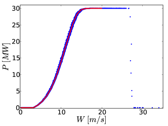
Figure 1: Rated power output $P$ vs. wind speed $W$ at site $\#15414$ for year 2004. Blue dots represent instantaneous measurements while the red curve represents power data filtered with a top-hat filter of width $\Delta_{W}=0.05$ [m/s], and interpolated via cubic splines.

For each site, wind speed and power data is available at 10 minute intervals for the years 2004 through 2006. Fig. 1 shows a scatter plot of rated power output vs. wind speed at wind site #15414. The rated power output is zero for wind speeds smaller than a threshold value of approximately 3.2 m/s. At speeds greater then approximately 26 m/s the generators are turned off, for safety reasons.

We take the following steps to post-process the NREL wind data into wind samples for use in our SED model:

1. Construct hourly averages for the wind speed; consider wind speed data for each day to be an independent sample from a 24-dimensional random field.

2. Choose a range of dates and assemble a set of 24-dimensional samples from this date range. For example, considering the month of January for 2004 through 2006 leads to 93 samples. This step was adopted to account for seasonal changes in wind patterns.

Fig. 2 shows select daily log-transformed ($W_{L}=\log(W)$) wind speed samples at site $\#15414$. We adopted this transformation to ensure positivity of wind speed samples, generated via the algorithm described below.

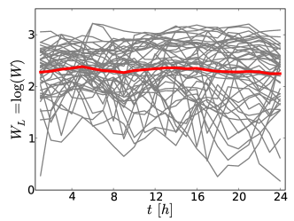
Figure 2: Select daily wind data from January 2004-2006 at site $\#15414$. The red curve corresponds to the mean of these daily samples.

We represent $W_{L}$ via a KL expansion

$$W_{L}(t,\omega)=\left<W_{L}(t,\omega)\right>+\sum_{k=1}^{\infty}\sqrt{\lambda_{k}}f_{k}(t)\xi_{k}(\omega)$$ (5)

where $\left<W_{L}(t,\omega)\right>$ denotes the mean of $W_{L}(t,\omega)$, $f_{k}(t)$ and $\lambda_{k}$ are respectively eigenfunctions (eigenvectors in a discrete setting) and eigenvalues of the covariance matrix $\Sigma_{W_{L}}$ of $W_{L}(t,\omega)$, and $\xi_{k}$ denotes uncorrelated random variables with zero mean and unit variance. Projecting realizations of $W_{L}$ onto $f_{k}$ leads to samples of $\xi_{k}$. These samples are generally not independent. In the special case where $W_{L}$ is a Gaussian random process, $\xi_{k}$ are i.i.d. standard normal random variables.

If known, the covariance matrix $\Sigma_{W}$ can be specified analytically. Otherwise, if sufficient samples are available, the covariance matrix can also be estimated from these realizations. For In our experiments, we estimate the covariance matrix using daily samples for select times of the year during 2004-2006. Once the covariance matrix is available, the eigenvalues and eigenvectors in Eq. (5) are given by solutions of the Fredholm equation of second kind

$$\int\Sigma_{W_{L}}(t,s)f(s)\,ds=\lambda f(t).$$

We discretize and solve this equation using the Nyström method [15], considering a mid-point quadrature rule to integrate over the discrete 24-hour period.

Fig. 3 shows the mean and first few KL modes corresponding to the month of January at the three wind sites considered in this study. The large degree of similarity for the KL modes between the three sites suggest a similar structure for the time correlations in the wind speed. We will further explore the structure of the covariance matrices $\Sigma_{W}$ in Section III-B.

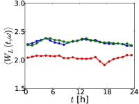
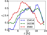
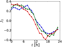
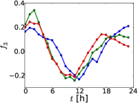
Figure 3: The mean, $\left<W_{L}(t,\omega)\right>$, and first three eigenvectors, $f_{1}$, $f_{2}$, and $f_{3}$, at several wind sites based on data from January 2004-2006.

Because the stochastic dimensions are uncorrelated, the total variance of the stochastic process is given as the sum of variances from individual KL mode, as follows:

$$\textrm{Var}\left[W_{L}(t,\omega)\right]=\sum_{k=1}^{24}\lambda_{k}f_{k}^{2}(t)\underbrace{\textrm{Var}[\xi_{k}]}_{=1}.$$

Given that eigenvectors are orthonormal with respect to the deterministic space (the discretized time axis in our study), it follows that:

$$\int_{T}\textrm{Var}[W_{L}(t,\omega)]dt=\sum_{k=1}^{24}\lambda_{k}.$$ (6)

As a result, an N-truncated expansion, $N\leq 24$, will explain

$$100\times\left(\sum_{k=1}^{N}\lambda_{k}\right)\Bigg{/}\left(\sum_{k=1}^{24}\lambda_{k}\right)\,[\%]$$ (7)

of the total variance of the random field. Fig. 4 shows the dependence of the fractional variance given in Eq. (7) on the number of terms $N$ in the truncated KL expansions at the three wind sites. It is evident that for all sites, $N=6$ modes are sufficient to capture approximately $95\%$ of the total variance in the daily wind profiles.

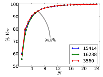
Figure 4: Percentages of the total variance explained by truncated KL expansions with an increasing number of modes, for our three wind sites.

We also examine the re-construction of select daily wind samples with truncated KL expansions, shown in Fig. 5. The results indicate that $N=6$ KL modes are sufficient to represent most of the daily variability. Similar results are observed for other, randomly selected, samples.

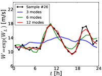
Figure 5: Reconstruction of daily wind samples via truncated KL expansion. Left plot corresponds to Jan 1, 2004 and the right plot to Jan 26, 2004.

Next, we test the degree of dependence between KL random variables. We start by constructing empirical cumulative distribution functions (CDFs) from RV samples. These samples are obtained by projecting each daily wind speed sample onto the corresponding KL mode. Fig. 6 shows the empirical CDFs for $\xi_{1}$ through $\xi_{15}$ at two select wind sites. Visual inspection of these results and comparison with the CDF of a standard normal RV indicate strong similarities. Because these RVs are uncorrelated by construction, modeling them as standard normals implies that they are also independent.

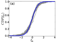
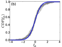
Figure 6: Empirical CDFs (depicted in gray) for $\xi_{1}$ through $\xi_{15}$ at (a) site 16238 and (b) site 3560. The CDF for a standard normal random variable is shown in blue, for reference.

We further investigate relationships among the standard normal RVs across the sites we consider in our experiments. To this end we employ distance correlation factors [16, 17] between pairs of RVs corresponding to the same KL mode at different sites. These factors are shown in Table I. Smaller values, towards zero, indicate negligible dependence between pairs of RVs, while larger values, close to 1, indicate a strong dependence. These results indicate a strong correlation between sites $\#15414$ and $\#16238$ for the first two KL modes, while the same KL mode at site $\#3560$ shows little correlation with the first two sites. The third and fourth RVs, as well as the other RVs (not shown), show little correlation between sites. This is somewhat to be expected given the nature of turbulence. Specifically, low KL modes are associated with large scale structures which are likely similar if sites are geographically situated, while higher order KL modes are associated with smaller scale structures with much faster eddy turnover times.

TABLE I: Distance correlation factors for $\xi_{1}$ - $\xi_{4}$ between wind sites.

RV	16238-15414	16238-3560	15414-3560
$\xi_{1}$	0.91	0.24	0.24
$\xi_{2}$	0.84	0.13	0.18
$\xi_{3}$	0.67	0.18	0.19
$\xi_{4}$	0.53	0.23	0.22

In experiments described below, we consider a stochastic space with $N=6$ dimensions at each site. Given that we model the first two modes at two sites as dependent, the total dimensionality of the stochastic space is $3\times 6-2=16$. Given the representation of daily wind profiles as truncated KL expansions, it follows that renewable generation $p_{r}^{t}({\bm{\xi}})=f(\exp(W_{L}(t,{\bm{\xi}}))$ is a function on the same stochastic space. We neglect the (small) noise in the conversion of wind speed into power and approximate $f$ as a cubic spline interpolation through the filtered rated power data. This approximation is depicted by the red line in Fig. 1.

III-B Wind Power Forecast Models

In this section we discuss the algorithm for generating wind power scenarios for day-ahead economic dispatch studies. We employ the KLE approach described in the previous section, with the covariance matrix adjusted to account for typical uncertainties of wind speed data obtained from weather forecast moedls.

We first start by fitting a functional form through the covariance matrix corresponding to each site. Fig. 7 shows, with thin grey lines, a typical decay in the components of $\Sigma_{W}$ with increasing time lag. We model this data with a Matern covariance kernel [18]

$$\overline{\Sigma}_{W}(\Delta t)=\frac{2^{1-\nu}}{\Gamma(\nu)}\left(\frac{\sqrt{2\nu}\Delta t}{l_{t}}\right)K_{\nu}\left(\frac{\sqrt{2\nu}\Delta t}{l_{t}}\right).$$ (8)

Here, $\nu$ and $l_{t}$ are positive parameters, $\Gamma(\cdot)$ is the gamma function, and $K_{\nu}(\cdot)$ is the modified Bessel function of the second kind. The Matern kernel offers more flexibility for modeling covariances compared to, for example, exponential and square exponential forms which are particular cases of the Matern kernel, for $\nu=1/2$ and $\nu\rightarrow\infty$, respectively.

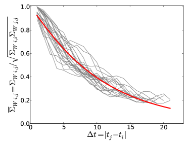
Figure 7: Decay of covariance matrix $\Sigma_{W}$ components, shown with thin grey lines, with increasing time lag $\Delta t=|t_{j}-t_{i}|$, anchored at several time instances $i$ for site #16238. Values are normalized by the diagonal entries. Matern covariance model is shown with blue line.

Table II shows the parameters of the Matern kernels for the three sites employed in this study. We obtain similar values for the two sites (15414 and 16238) that are geographically close. Furthermore, the values for the $\nu$ parameter for these two sites are close to $\nu=1/2$ indicating covariance matrices that are close to exponential form.

TABLE II: Parameters of Matern kernels corresponding to select wind sites.

Wind Site	$l_{t}$	$\nu$
$15414$	11.40	0.56
$16238$	11.15	0.57
$3560$	9.79	0.78

Next we estimate the magnitude of the variance in the estimates of wind magnitude. Since data on wind forecast and actual realizations were not immediately available to us, we proceeded to estimate uncertainty in the wind forecasts given available data for wind power. Specifically, we used data for day-ahead forecast and actual realizations obtained from Belgium Electricity Grid Operator ELIA [19]. We considered the aggregate wind power values for the land-based wind farms and computed the standard deviation for hourly wind power output based on data for years 2012 through 2015. We found a relative value of about $\sigma_{P}=35\%$. Further, this value is independent of the time of the day for the day-ahead forecasts.

Based on the formulations presented in this section we employ the following algorithm to generate wind power samples that are consistent to historical wind characteristics at the selected wind sites:

1. Forecast day-ahead wind profiles at selected wind sites.

2. Using $\sigma_{P}$ defined above, estimate a mean $\sigma_{W}$ based on the mean forecast wind speed and the rated power output curves for each site, similar to the one presented in Fig. 1.

3. Construct covariance matrix, ${\Sigma}_{W}=\sigma_{W}^{2}\overline{\Sigma}_{W}$, where $\overline{\Sigma}_{W}$ is the normalized Matern covariance expression presented in Eq. (8).

4. Perform eigen-decomposition for $\Sigma_{W}$ and generate wind samples via Eq. (5) for select samples of $\bm{\xi}$.

5. Convert wind samples into wind power values, see Fig. 1.

IV Accurate estimation of expected cost with limited samples

We now return to the evaluation of the expected cost in Eq. (1) corresponding to the ED problem in Eqs. (2) and (3). We can estimate the expected production cost by using a finite number of renewable power realizations (i.e., scenarios) $s\in\mathcal{S}$ sampled from the joint density $PDF({\bm{\xi}})$. For our current example, each $\xi$ is a standard normal RV, hence the sampling can be done independently in each stochastic direction. Defining $\rho\equiv 1/|\mathcal{S}|$, where $|\mathcal{S}|$ is the cardinality of $\mathcal{S}$, the stochastic ED in Eq. (1) can be rewritten as:

$$\min_{\bm{f,p,q,\theta}}\quad \rho\sum_{s\in\mathcal{S}}Q(\bm{x},s)$$ (9)

where $Q(\bm{x},s)$ is the solution of Eqs. (2) and (3) for a particular instance of the renewable generation $p_{r}^{t}({\bm{\xi}})\rightarrow p_{r}^{t}(s)$.

Formulation (9) represents an extensive form of the stochastic ED problem, based on $|\mathcal{S}|$ sampled scenarios from the stochastic space corresponding to wind power generators. The typical scenario sampling approach described above uses Monte Carlo (MC) sampling to approximate an integration, thereby estimating an expectation. While MC algorithms are commonly used for their convenience and robustness, their poor convergence rate is well-known. The MC estimate of the expectation has error

$$\mathrm{V}[Q({\bm{x}},{\bm{\xi}})]/\sqrt{|S|},$$ (10)

where $\mathrm{V[Q]}$ denotes the variance of the RV $Q$. Given the significant additional complexity incurred by including stochasticity in the optimization problem, a stochastic formulation becomes advantageous relative to a deterministic formulation when the variance is large. Hence, accurate estimation of the expectation is not only an academic exercise but is important in practice.

According to Eq. (10), accurate estimation can be achieved by increasing the number of samples. However, a linear decrease in error requires a quadratic increase in the number of samples, which can quickly render the stochastic optimization problem intractable. This illustrates the limitation of MC algorithms in providing accurate estimations; while they are convenient, they are not efficient.

We propose a method based on Polynomial Chaos expansions that can enable high precision quantification of uncertainties with fewer samples. In the following sections, we will first outline the Polynomial Chaos expansion construction and then present its implementation for the ED problem.

IV-A Representation of uncertainty using Polynomial Chaos

Given the formulation in Eq. (3) with uncertain/random loads leading to uncertain/random production costs, we employ efficient UQ methods that rely on functional representations of random variables. Specifically, we use Polynomial Chaos (PC) expansions. A brief description of PC is presented below. For an in-depth description, the reader is referred to a series of publications on this topic [20, 11, 21, 22].

We begin by setting up a requisite theoretical framework as follows. Define the probability space $(\Omega,\mathfrak{S},P)$, where $\Omega$ is a sample space, $\mathfrak{S}$ is a $\sigma$-algebra on $\Omega$, and $P$ is a probability measure on $(\Omega,\mathfrak{S})$. Further, defining the germ ${\bm{\xi}}=\{\xi_{1},\xi_{2},\ldots,\xi_{n}\}$ as a set of independent identically distributed (iid) RVs in $L_{2}(\Omega,\mathfrak{S},P)$, to be further specified below, we focus on the probability space $(\Omega,\mathfrak{S}_{\bm{\xi}},P)$ employing the sigma algebra generated by ${\bm{\xi}}$. In this framework, any RV $X:\Omega\rightarrow\mathbb{R}$, where by construction $X\in L_{2}(\Omega,\mathfrak{S}_{\bm{\xi}},P)$, can be written as a PC expansion (PCE):

$$X(\omega)=X({\bm{\xi}}(\omega))=\sum_{k=0}^{\infty}\alpha_{k}\Psi_{k}({\bm{\xi}})$$ (11)

where the basis functions $\Psi_{k}$ are multivariate polynomials that are orthogonal, by construction, with respect to the density of ${\bm{\xi}}$. Thus

$$\langle\Psi_{i}\Psi_{j}\rangle=\int\Psi_{i}(\xi)\Psi_{j}(\xi)dP(\xi)=\delta_{ij}\langle\Psi_{i}^{2}\rangle$$ (12)

where $\delta_{ij}$ is Kronecker’s delta. Further, given this orthogonality, we have

$$\alpha_{k}=\frac{\langle X\Psi_{k}\rangle}{\langle\Psi_{k}^{2}\rangle}$$ (13)

where the inner product is defined, for any RV $Z({\bm{\xi}})$, by the Galerkin projection

$$\langle Z\rangle=\int Z({\bm{\xi}})p_{\bm{\xi}}({\bm{\xi}})d{\bm{\xi}}.$$ (14)

Moreover, the $\Psi_{k}$ are products of univariate polynomials, namely $\Psi_{k}({\bm{\xi}})=\psi_{k_{1}}(\xi_{1})\cdots\psi_{k_{n}}(\xi_{n})$. In a practical computational context, one truncates the PCE to order $p$. The number of terms in the resulting finite PCE

$$X\approx\sum_{k=0}^{P}\alpha_{k}\Psi_{k}({\bm{\xi}})$$ (15)

is given by $P+1={(n+p)!}/{n!p!}$. We dispense with the $\approx$ symbol in the remainder of this paper, employing for any RV $X({\bm{\xi}})$ its truncated PCE

$$X=\sum_{k=0}^{P}\alpha_{k}\Psi_{k}({\bm{\xi}}).$$ (16)

Generalized PC (gPC) expansions have been developed by Xiu and Karniadakis [22] using a broad class of orthogonal polynomials in the “Askey” scheme [23]. Each family of polynomials corresponds to a given choice of distribution for the $\xi_{i}$ and is, by construction, orthogonal with respect to the density of $\xi_{i}$. In general, the most useful choices for $({\bm{\xi}},\Psi)$ are normal RVs with Hermite polynomials and uniform RVs with Legendre polynomials.

IV-B Construction of PCE for the Minimum Cost

In the context of this study with uncertain renewable wind generation dependent on a stochastic space of iid standard normal random variables, ${\bm{\xi}}=\{\xi_{1},\xi_{2},\ldots,\xi_{n}\}$, we employ Hermite polynomials to construct a Hermite-Gauss (HG) PCE for the (minimum) cost $Q(\bm{x},{\bm{\xi}})$. We employ Eq. (16) for a truncated HG PCE

$$Q_{\mathrm{PC}}({\bm{x}},{\bm{\xi}})=\sum_{k=0}^{P}c_{k}({\bm{x}})\Psi_{k}({\bm{\xi}}),$$ (17)

where $\Psi_{k}({\bm{\xi}})$ are $n$-variate Hermite polynomials. The coefficients $c_{k}$ depend on the discrete variable $\bm{x}$, hence separate PCE approximations for $Q$ will be constructed for each instance of $\bm{x}$ chosen in the unit commitment stage. Given Eq. (14), we have

$$c_{k}(\bm{x})=\frac{\langle Q\Psi_{k}\rangle}{\langle\Psi_{k}^{2}\rangle}=\frac{1}{\langle\Psi_{k}^{2}\rangle}\int_{\mathfrak{R}^{n}}Q(\bm{x},{\bm{\xi}})\Psi_{k}({\bm{\xi}})p({\bm{\xi}})\,d{\bm{\xi}}.$$ (18)

where we have used $p({\bm{\xi}})$ as a product of univariate standard normal PDFs. The dimensionality of the PCE in Eq. (17) is the same as the number of stochastic dimensions used to represent the uncertain renewable power. For the study presented in this paper, $n=16$.

Given $Q_{\mathrm{PC}}({\bm{x}},{\bm{\xi}})$, then, we have

$${\overline{Q}}(\bm{x})=\mathrm{E}_{\bm{\xi}}[Q(\bm{x},{\bm{\xi}})]=\langle Q(\bm{x},{\bm{\xi}})\rangle=c_{0},$$ (19)

being the solution of the stochastic ED problem. The PCE in Eq. (17) can also be used to generated higher-order moments for the minimum cost, based directly on the coefficients for the corresponding PC basis terms.

Several methods can be employed to evaluate the projection integrals in Eq. (18). MC methods can be used in principle, but are impractical given their slow convergence rate. Alternatively, for smooth integrands, and particularly in low-moderate dimensional problems, sparse quadrature methods [24, 25, 26] can provide highly accurate results with smaller numbers of deterministic samples.

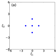
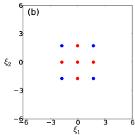
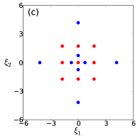
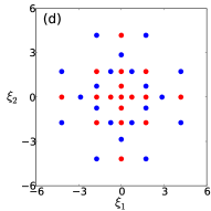
Figure 8: Placement of deterministic samples via a sparse grid approach: (a) Level 1, (b) Level 2, (c) Level 3, and (d) Level 4. For Levels 2 through 4, the red symbols show samples for previous levels while blue symbols show newly added samples.

Fig. 8 shows, in a 2D configuration, the locations of deterministic samples we use, with a sparse grid employing Gauss-Kronrod quadrature [27]. Several levels are shown in the figure, starting with the first level in Fig. 8(a), and following with additional samples leading to Levels 2, 3, and 4, in Fig. 8(b)-(d). A first order PCE requires a Level 2 sparse grid, while a second order PCE requires a Level 3 grid. The number of requisite samples using sparse-quadrature evaluation of the projection integrals, for a given requisite surrogate accuracy, is much smaller than the corresponding number of MC samples, as we will illustrate in the next subsection.

IV-C Numerical Results

We now present numerical results comparing the expected costs of our SED model using scenarios obtained with both our Polynomial Chaos approach to sampling versus a traditional Monte Carlo approach. We consider the IEEE 118-bus test system [28] augmented with the three wind generation sites discussed in Section III. The three renewable generators at sites 15414, 16238, and 3560 replace the conventional generators at buses 89, 69, and 10, respectively. We employ $|T|=24$ time periods and represent stochastic renewable generation via the Karhunen-Loeve expansions presented in Section III. We use 6 KL modes per site. Given the strong dependence between the first two RVs for sites 15414 and 16238, the effective dimensionality of the system decreases by 2, to a total of 16.

We first explore the dependence of $Q({\bm{x}},{\bm{\xi}})$ on the stochastic space that characterizes renewable generation. Fig. 9 shows 2D slices through the 16D ${\bm{\xi}}$ space. All slices are anchored at the origin ${\bm{\xi}}=0$. RVs $\xi_{1}$ through $\xi_{6}$ correspond to site 16238, while $\xi_{1}$, $\xi_{2}$, and $\xi_{7}$ - $\xi_{10}$ correspond to site 15414. The remaining random variables, $\xi_{11}$ - $\xi_{16}$, correspond to site 3560. The expected cost is about $\$2.4$ million, and the relative change about the mean is about $15\%$ in the numerical tests presented here. The results shown in the top row of Fig. 9 indicate that $Q$ is strongly dependent on $\xi_{1}$, while the dependence on $\xi_{2}$ and $\xi_{3}$ is weaker – as suggested by negligible contour changes in those directions. The slice in the $(\xi_{1},\xi_{11})$ plane highlights the contribution of $\xi_{11}$ to the variation of $Q$, while the slice in the $(\xi_{11},\xi_{12})$ plane indicates less impact of the second mode for site 3560 on cost. Other 2D slices (not shown) confirm the diminishing impact that higher-order modes have on $Q$. Collectively, these results also indicate that $Q({\bm{x}},{\bm{\xi}})$ is smooth in ${\bm{\xi}}$, which makes it amenable to a PCE representation.

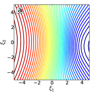
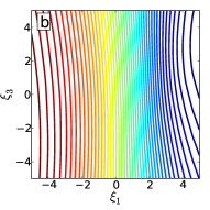
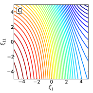
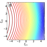
Figure 9: Two dimensional slices through the center of the stochastic space, ${\bm{\xi}}=0$. Random variables corresponding to (a) first two modes for Wyoming sites, (b) 1st and 3rd mode for WY sites, (c) first modes for WY and CA sites, and (d) first two modes for CA site. The countour lines correspond to iso-levels of $Q$, increasing from blue to yellow to red.

We next proceed to test the accuracy of the PCE representation for $Q({\bm{x}},{\bm{\xi}})$ with respect to actual model evaluations. We construct several PCEs, from 1st to 4th order. Given the 16-dimensional stochastic space corresponding to the three wind sites, the number of sparse quadrature sample points necessary for the construction of the PCE coefficients is approximately $5\times 10^{2}$ for a 1st order expansion, $5\times 10^{3}$ for a 2nd order expansion, $3.6\times 10^{4}$ for a 3rd order expansion, and $2\times 10^{5}$ for a 4th order expansion. We cross-validate our PCE representations relative to exact solutions at $5\times 10^{5}$ randomly chosen ${\bm{\xi}}$ samples. Fig. 10 shows the relative $L_{1}$ error between actual model evaluations and the PCE-approximated cost. This error is relative to the expected minimum cost computed using all model evaluations available and is converted to percentages. For brevity, only a random subset of $2\times 10^{4}$ samples are shown.

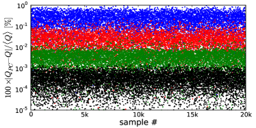
Figure 10: Cross-validation of PCE approximation for the minimum cost $Q({\bm{x}},{\bm{\xi}})$. The blue, red, green, and black symbols correspond to 1st through 4th order PCEs.

These results indicate a drop of about one order of magnitude, per polynomial degree, for the magnitude of the error between full model evaluations and the PCE results.

The above analysis explores the dependence of minimum cost for individual samples on the stochastic space corresponding to the uncertain wind at select sites, and the accuracy of the PCE approach in capturing this dependence. However, in the context of the SED problem, and for the present work in particular, we are only interested the accuracy of the expected minimum cost $\left<Q({\bm{x}},{\bm{\xi}})\right>$. Hence, our goal here is to demonstrate the efficiency of a quadrature approach to estimate the expectation.

Toward this goal, we show the convergence of $\left<Q({\bm{x}},{\bm{\xi}})\right>$ as a function of the number of samples considered. For the PCE approach, the expected minimum cost is simply given by the $c_{0}$ coefficient in Eq. (18). The results shown with blue are based on this coefficient, computed with increasingly accurate sparse quadratures. The error measure is relative, being normalized with respect to the value corresponding to the next higher accuracy result, defined as

$$E_{PC,i}=\frac{|{{c_{0}}}_{i}-{{c_{0}}}_{i+1}|}{{{c_{0}}}_{i+1}}$$ (20)

where the subscript $i$ denotes the quadrature level, e.g., $33$ model evaluations for level $1$, $513$ model evaluations for level $2$, and so forth. The error for the MC results is computed using a similar approach. However, because results for the MC approach depend on a randomly drawn set of samples, we show results for several realizations. The specific formula is given as

$$E_{MC,i}^{j}=\frac{|\overline{Q}_{i}^{j}-\overline{\overline{Q}}_{i+1}|}{\overline{\overline{Q}}_{i+1}}$$ (21)

where the subscript $i$ denotes the number of samples used to compute the average cost $\overline{Q}_{i}^{j}$, e.g., 10 samples for $i=1$, 100 samples for $i=2$, etc. We employed 10 realizations, indexed by superscript $j$, for each set of MC samples; the average cost over all realizations is denoted using a double overline. $E_{MC,i}^{j}$ is shown with red circles in Fig. 11, while the red line connects the mean error over all realizations for a particular number of MC samples. The dashed lines show power-law curve fits, $a\times N^{-b}$, for the data, which we use to analyze convergence rates as a function of the number of samples. For the MC approach we recover the theoretical convergence rate, $b=0.5$, while for the PCE approach $b=1.9$. Visual inspection of the PCE results and power law fits indicate a stronger polynomial convergence rate than MC, rather than an exponential rate (results not shown) corresponding to spectral accuracy.

In this figure a $1\%$ error level corresponds to about $\$24$K, while a $0.01\%$ error level is in the hundreds of dollars. These results indicate that if a low degree of accuracy, e.g. $1\%$, is sufficient or desired, then the PCE approach exhibits a computational cost that is comparable to the MC approach. Nevertheless there is a considerable spread in the accuracy of these estimates, making MC estimates with a small number of samples somewhat unreliable. For situations where higher accuracies are required, for example of $0.01\%$, the PCE estimates require one to two orders of magnitude less model evaluations compared to the MC estimates.

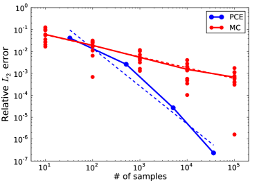
Figure 11: Comparison of errors in the estimation of expected cost between PCE-based results and Monte Carlo estimates. Dashed lines show power-law fits, $a\times N^{b}$ to test the convergence rates of the MC and PCE approaches.

V Conclusion

In this paper, we present methods for efficient representation of uncertainty, with emphasis on the Stochastic Economic Dispatch problem. We present two, related, category of methods, one for spectral random fields representations, and one for functional representation of random variables.

In the first part of this paper we employ data on renewable wind generations provided by NREL. We determine that 24-hour wind samples can be represented via Karhunen-Loeve (KL) expansions. This expansion represents stochastic processes by a linear combination of orthogonal modes. Further, the KL representation employs the basis that provides the minimum total $L_{2}$ error. Analysis of the KL eigenspectra at several wind sites indicate that $6$ KL modes are sufficient to capture about $95\%$ of the total variance, effectively reducing the dimensionality of the stochastic space by a factor of $4$. The dimensionality of the stochastic space is further reduced by exploiting the dependence between KL random variables for wind sites that are geographically close.

In the second part of the paper we present an approach to reduce the computational cost associated with stochastic unit commitment and economic dispatch, by reducing the number of required forecast samples. This approach is based on Polynomial Chaos expansion (PCE) models for the production cost that cover the uncertainty in the renewable generation. The construction of the PCE terms is based on the projection of the model on increasingly higher basis modes. Consequently, the global error in an $L_{2}$ sense between the surrogate model and the actual simulations is easily controlled.

We present computational results for the 118-bus test case, augmented to account for renewable generation. We find that quadratic PCE models for the production cost showed pointwise relative errors less than $1\%$ throughout the uncertain demand space. For relative accuracies of $o(10^{-4})$, the PCE approach is one to two orders of computationally more efficient compared to Monte Carlo estimates.

We plan to extend the methods presented here to higher-dimensional power grid problems. In order to alleviate the curse of dimensionality in such studies we plan to emply global sensitivity analysis to eliminate the stochastic variables that are not important for the expected cost. And based on results observed in this paper, we plan to explore adaptive sparse quadrature constructions to tailor of the PCE order to the specific dependence of minimum cost on each component of the stochastic space.

Appendix. Total Variance of Karhunen-Loeve Expansion

Starting from Eq. (5), it follows that

$$\textrm{Var}[W_{L}(t,\omega)]=\textrm{Var}\left[\sum_{k=1}^{24}\sqrt{\lambda_{k}}f_{k}(t)\xi_{k}\right]$$

Here, we converted the infinite sum into one over the $24$ modes that can be extracted from 24h wind samples. As noted in Section III, $\xi_{k}$ are uncorrelated random variables with zero mean and unit variance. To simplify notation, in this Appendix, we change notation and denote the product $\sqrt{\lambda_{k}}\xi_{k}$ as $X_{k}$. This new set of RVs are uncorrelated with zero mean and variance $\lambda_{k}$.

The variance of the rhs of the expression above can be written as

For uncorrelated random variables $X_{i}$, $X_{j}$, the expectation in the second sum in Eq. (LABEL:eq:vsum2) is identically zero, $\mathbb{E}\left[\left(X_{i}-\mathbb{E}\left[X_{i}\right]\right)\left(X_{j}-\mathbb{E}\left[X_{j}\right]\right)\right]=0$. Making use of $\textrm{Var}[X_{k}]=\lambda_{k}$, it follows that

$$\textrm{Var}\left[\sum_{k}f_{k}(t)X_{k}\right]=\sum_{k}f_{k}^{2}(t)\textrm{Var}[X_{k}]=\sum_{k}f_{k}^{2}(t)\lambda_{k}$$ (25)

The total variance over the entire deterministic space is given by

$$\int_{t}\textrm{Var}\left[\sum_{k}f_{k}(t)X_{k}\right]dt=\int_{t}\sum_{k}f_{k}^{2}(t)\lambda_{k}dt$$

Given that modes $f_{k}$ are orthonormal over the deterministic space, total variance of the KL expansion is given by

$$\int_{t}\textrm{Var}\left[W_{L}(t,\omega)\right]dt=\sum_{k}\lambda_{k}$$

References

- [1] M. Carrión and J. M. Arroyo, “A computationally efficient mixed-integer linear formulation for the thermal unit commitment problem,” IEEE Transactions on Power Systems, vol. 21, no. 3, pp. 1371–1378, 2006.
- [2] “ISO New England: Forecast and scheduling reserve adequacy analysis ,” www.iso-ne.com/support/training/courses/wem101/ 10_forecast_scheduling_callan.pdf, accessed: 2014-05-19.
- [3] P. A. Ruiz, R. C. Philbrick, E. Zack, K. W. Cheung, and P. W. Sauer, “Uncertainty management in the unit commitment problem,” IEEE Transactions on Power Systems, vol. 24, no. 2, pp. 642–651, 2009.
- [4] S. Takriti, J. Birge, and E. Long, “A stochastic model for the unit commitment problem,” IEEE Transactions on Power Systems, vol. 11, no. 3, pp. 1497–1508, 1996.
- [5] A. Papavasiliou and S. S. Oren, “Multiarea Stochastic Unit Commitment for High Wind Penetration in a Transmission Constrained Network,” Operations Research, vol. 61, no. 3, pp. 578–592, 2013.
- [6] Q. Wang, J. Wang, and Y. Guan, “Stochastic unit commitment with uncertain demand response,” IEEE Transactions on Power Systems, vol. 28, no. 1, pp. 562–563, 2013.
- [7] R. L.-Y. Chen, N. Fan, A. Pinar, and J.-P. Watson, “Contingency-constrained unit commitment with post-contingency corrective recourse,” Annals of Operations Research, pp. 1–27, 2014.
- [8] D. Bertsimas, E. Litvinov, X. A. Sun, J. Zhao, and T. Zheng, “Adaptive robust optimization for the security constrained unit commitment problem,” IEEE Transactions on Power Systems, vol. 28, no. 1, pp. 52–63, 2013.
- [9] F. B. Thiam and C. L. DeMarco, “Optimal transmission expansion via intrinsic properties of power flow conditioning,” in 2010 North American Power Symposium (NAPS), 2010, pp. 1–8.
- [10] H. N. Najm, “Uncertainty Quantification and Polynomial Chaos Techniques in Computational Fluid Dynamics,” Annual Review of Fluid Mechanics, vol. 41, no. 1, pp. 35–52, 2009.
- [11] R. G. Ghanem and P. D. Spanos, Stochastic Finite Elements: A Spectral Approach. Springer Verlag, New York, 1991.
- [12] C. Safta, R. L.-Y. Chen, H. Najm, A. Pinar, and J.-P. Watson, “Toward using surrogates to accelerate solution of stochastic electricity grid operations problems,” in North American Power Symposium (NAPS), 2014, Sept 2014, pp. 1–6.
- [13] O. Le Maître and O. Knio, Spectral Methods for Uncertainty Quantification. New York, NY: Springer, 2010.
- [14] “NREL: Transmission Grid Integration - Western Wind Dataset,” http://www.nrel.gov/electricity/transmission/wind_integration_dataset.html, accessed: 2015-02-28.
- [15] E. J. Nyström, “Über die praktische auflösung von integralgleichungen mit anwendungen auf randwertaufgaben,” Acta Mathematica, vol. 54, no. 1, pp. 185–204, 1930.
- [16] G. J. Székely, M. L. Rizzo, and N. K. Bakirov, “Measuring and testing dependence by correlation of distances,” Annals of Statistics, vol. 35, pp. 2769–2794, 2007.
- [17] C. Safta, K. Sargsyan, H. N. Najm, K. Chowdhary, B. Debusschere, L. P. Swiler, and M. S. Eldred, “Probabilistic Methods for Sensitivity Analysis and Calibration of Computer Models in the NASA Challenge Problem,” Journal of Aerospace Information Systems, 2015, in press.
- [18] C. E. Rasmussen and C. K. I. Williams, Gaussian Processes for Machine Learning. MIT Press, 2006.
- [19] “ELIA: Wind-Power Generation Data,” http://www.elia.be/en/grid-data/power-generation/wind-power, accessed: 2015-07-26.
- [20] N. Wiener, “The homogeneous chaos,” Am. J. Math., vol. 60, pp. 897–936, 1938.
- [21] S. Janson, Gaussian Hilbert Spaces. Cambridge, UK: Camb. Univ. Press, 1997.
- [22] D. Xiu and G. E. Karniadakis, “The Wiener-Askey polynomial chaos for stochastic differential equations,” SIAM Journal on Scientific Computing, vol. 24, no. 2, pp. 619–644, 2002.
- [23] R. Askey and J. Wilson, “Some basic hypergeometric polynomials that generalize jacobi polynomials,” Memoirs Amer. Math. Soc., vol. 319, pp. 1–55, 1985.
- [24] S. A. Smolyak, “Quadrature and interpolation formulas for tensor products of certain classes of functions,” Soviet Mathematics Dokl., vol. 4, pp. 240–243, 1963.
- [25] T. Gerstner and M. Griebel, “Numerical integration using sparse grids,” Numerical Algorithms, vol. 18, pp. 209–232, 1998.
- [26] P. Conrad and Y. Marzouk, “Adaptive smolyak pseudospectral approximations,” SIAM Journal on Scientific Computing, vol. 35, no. 6, pp. A2643–A2670, 2013.
- [27] T. Patterson, “The optimum addition of points to quadrature formulae,” Mathematics of Computation, vol. 22, no. 104, pp. 847–856, 1968.
- [28] “Power Systems Test Case Archive ,” http://www.ee.washington.edu/research/pstca/, accessed: 2014-05-01.