Infrared spectral properties of M giants

Abstract

We observed a sample of 20 M giants with the Infrared Spectrograph on the Spitzer Space Telescope. Most show absorption structure at 6.6–6.8 $\mu$m which we identify as water vapor, and in some cases, the absorption extends from 6.4 $\mu$m into the SiO band at 7.5 $\mu$m. Variable stars show stronger H₂O absorption. While the strength of the SiO fundamental at 8 $\mu$m increases monotonically from spectral class K0 to K5, the dependence on spectral class weakens in the M giants. As with previously studied samples, the M giants show considerable scatter in SiO band strength within a given spectral class. All of the stars in our sample also show OH band absorption, most noticeably in the 14–17 $\mu$m region. The OH bands behave much like the SiO bands, increasing in strength in the K giants but showing weaker dependence on spectral class in the M giants, and with considerable scatter. An examination of the photometric properties reveals that the $V-K$ color may be a better indicator of molecular band strength than the spectral class. The transformation from Tycho colors to Johnson $B-V$ color is double-valued, and neither $B-V$ nor $B_{T}-V_{T}$ color increases monotonically with spectral class in the M giants like they do in the K giants.

1. Introduction

Red giants dominate the infrared skies (Grasdalen & Gaustad, 1971). Their brightness and prevalence have led to their frequent use as infrared standard stars. Originally, the spectra of these stars were assumed to be blackbodies in the mid-infrared (e.g. Gillett & Merrill, 1975), but they actually include strong molecular absorption bands. Spectra from the Kuiper Airborne Observatory revealed the presence of CO and SiO bands in the spectrum of $\alpha$ Tau and several other late-type giants (Cohen et al., 1992a, b). Red giants are also associated with mass-loss and dust production, and these molecules are precursors to the dust, adding to the importance of understanding their spectral properties.

Heras et al. (2002) used spectra from the Short-Wavelength Spectrometer (SWS) on the Infrared Space Observatory (ISO) to show that the strength of the CO and SiO bands increased with later spectral classes, but with significant scatter. The scatter is greater in the M giants than in the K giants, and it is greater for SiO than CO.

Sloan et al. (2015, hereafter Paper I) followed up with a study of 33 K giants observed by the Infrared Spectrograph (IRS; Houck et al., 2004) on the Spitzer Space Telescope (Werner et al., 2004). Wavelength coverage limited their study to the SiO fundamental at 8 $\mu$m, and for that band, the scatter persisted, even though the IRS sample was limited to a luminosity class of “III”, while the earlier SWS sample had included bright giants with classes “II” and “IIIa”.

The spectra of late-type giants can also show absorption from H₂O. Tsuji et al. (1997) detected H₂O at 6.7 $\mu$m in SWS spectra of giants of spectral class M2 and later. Tsuji (2001) identified several H₂O lines at $\sim$6.6 $\mu$m in stars as early as K5. Heras et al. (2002) examined a larger sample of SWS spectra and found that H₂O bands at 6.4–7.0 $\mu$m commonly appeared in all stars of spectral class $\sim$M2 or later. They were unable to diagnose any further dependencies with spectral class. Ardila et al. (2010) examined H₂O absorption in a sample observed with the IRS. They confirmed the presence of H₂O in M giants, suggesting a turn-on point at $\sim$M0, and found little variation in the band strength within the M giants.

OH is another absorber in the spectra of late-type giants. Van Malderen et al. (2004) identified several bands in the 14–20 $\mu$m region in spectra from the SWS. They found that the bands were stronger than predicted by models, but they were still too weak for more quantitative conclusions. The IRS sample of K giants confirmed that the observed bands were stronger than the models. The sample also shows that the bands grow stronger with later spectral class (Paper I).

To improve our understanding of how the SiO, H₂O, and OH bands behave with spectral class and build on what we have learned from previous observations of K giants with the IRS on Spitzer, we obtained infrared spectra of 20 M giants. Section 2 describes the sample and the spectra. Section 3 presents our analysis, and Section 4 discusses the results. We summarize our conclusions in Section 5. The Appendices detail how we determined the photometric properties of our sample and also describe our online spectroscopic data.

2. The sample

2.1. The IRS sample of M giants

We used several criteria to select the M giant sample observed with the IRS. We aimed to observe at least three stars in each spectral class from M0 to M6 in order to compare stars both within a given class and from one class to the next. The stars had to have photometry from the Infrared Astronomy Satellite (IRAS) at 12 and 25 $\mu$m consistent with a naked star. We excluded stars past M6 because they are usually associated with circumstellar dust.

All targets had to have a luminosity class of “III” and not classes like “IIIa” or “II–III”, which would indicate a difference in luminosity and surface gravity compared to the rest of the sample. And they could not be spectroscopic binaries or strong variables. This last constraint had to be relaxed somewhat, because some variability is typical at the latest spectral classes. Because most M6 giants are variables and dusty, we chose only two targets with this spectral class.

Table 1IRS sample of M giants

Target	Alias	RA	Declination	Spectral	Variability	$F_{12}$	AOR key
		(J2000)		Type	Class	(Jy)
HD 13570	$\cdots$	02 10 15.47	$-$61 05 49.1	M0 III	$\cdots$	0.89	21747456
HD 19554	$\cdots$	03 08 09.32	$-$19 18 10.6	M0 III	$\cdots$	1.31	21747712
HD 107893	NSV 19376	12 24 03.97	$-$26 00 50.4	M0 III	(NSV)	1.32	21747968
HD 17678	FM Eri	02 49 42.59	$-$17 16 47.3	M1 III	Lb:	1.12	21748224
BD+47 2949	HIP 97959	19 54 29.30	$+$47 54 49.7	M1 III	$\cdots$	1.27	21748480
HD 206503	$\cdots$	21 45 25.03	$-$67 06 12.8	M1 III	$\cdots$	0.92	21748736
HD 122755	V350 Hya	14 04 23.76	$-$29 53 58.7	M2 III	Lb	1.76	21748992
HD 177643	$\cdots$	19 10 54.20	$-$68 23 59.4	M2 III	$\cdots$	1.03	21749248
HD 189246	$\cdots$	20 00 41.66	$-$40 12 00.8	M2 III	$\cdots$	1.11	21749504
HD 26231	CZ Eri	04 07 23.80	$-$39 29 54.9	M3 III	SRb	1.20	21749760
HD 127693	$\cdots$	14 33 47.73	$-$40 01 18.0	M3 III	$\cdots$	0.75	21750016
HD 223306	DT Tuc	23 48 39.29	$-$59 03 27.2	M3 III	Lb:	0.72	21750272
HD 17766	XX Hor	02 48 26.35	$-$60 24 53.0	M4 III	Lb:	0.87	21750528
HD 32832	VX Pic	05 03 00.32	$-$54 05 52.8	M4 III	SRb	1.10	21750784
HD 46396	AX Dor	06 27 58.88	$-$66 45 15.9	M4 III	Lb:	1.53	21751040
HD 68422	V464 Car	08 08 48.91	$-$61 34 07.6	M5 III	Lb:	1.81	21751296
HD 74584	NSV 17963	08 41 07.97	$-$64 36 08.6	M5 III	(NSV)	1.67	21751552
HD 76386	CZ Lyn	08 57 12.10	$+$41 20 26.9	M5 III	SRb	2.51	21751808
HD 8680	BZ Phe	01 24 50.07	$-$42 45 51.9	M6 III	Lb:	0.88	21752064
BD+44 2199	BV CVn	12 31 59.43	$+$43 28 58.8	M6 III	Lb	2.95	21752320

Table 1 presents the sample in order of spectral class, which are from the Michigan catalogs of spectral classifications (Houk & Cowley, 1975; Houk, 1978, 1982; Houk & Smith-Moore, 1988), with three exceptions. Houk (1978) classified HD 8680 as M3 while Jones (1972) classified it as M6 III; we have adopted the latter because it includes a luminosity class. The first complete spectral type for BD+47 2949 appeared in the 1980 SAO catalog (Oschenbein, 1980). The classification for BD+44 2199 is from Upgren (1960).

In Table 1, the fraction of stars identified as definite variables increases with spectral class. Ardila et al. (2010) included one star from each spectral class in their Spitzer Atlas of Stellar Spectra, but they generally avoided the more variable sources. The infrared amplitudes are usually a small fraction of the optical amplitudes, typically one tenth or so (Smith et al., 2004; Price et al., 2010).

All 20 M giants were observed by the IRS as part of program 40112, in Cycle 4, between 2007 June and 2008 March. The observations used both the Short-Low (SL) and Long-Low (LL) modules, which obtain spectra with a resolution ($\lambda/\Delta\lambda$) of $\sim$60–120. All observations used the standard IRS nod sequence and integrated for 18 s per nod in SL and 28–60 s per nod in LL. Most of the observations were made with an offset peak-up star, which raises the odds of slight mispointings. The spectra were reduced identically to the K giants, and Paper I describes the methods of observation and reduction in more detail.

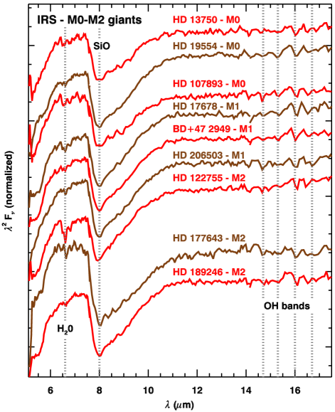
Figure 1.— IRS spectra of the early M giants (M0–M2), plotted in Rayleigh-Jeans units, so that a Rayleigh-Jeans tail would be a horizontal line. Vertical dotted lines mark the positions of the deepest absorption in the SiO fundamental at 8 $\mu$m, the H₂O absorption at 6.6 $\mu$m, and the strongest OH bands from 14.5 to 17 $\mu$m.

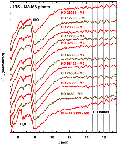
Figure 2.— IRS spectra of the late M giants (M3–M6), plotted and labeled as in Figure 1.

Figures 1 and 2 present the sample of M giants observed with the IRS, plotted in Rayleigh-Jeans units ($\lambda^{2}$$F_{\nu}$). In these units, the Rayleigh-Jeans tail of a Planck function would be a horizontal line and a typical stellar continuum would rise to longer wavelengths, asymptotically approaching the Rayleigh-Jeans limit.

Some of the spectra do not conform to this expected shape, most notably HD 177643 (M2) in Figure 1, with the continuum at 6–7.5 $\mu$m greater than at 12 $\mu$m and beyond. This misbehavior arises when the telescope is slightly mispointed, so that the source is not properly centered in the slit. Generally, the slit throughput is a function of wavelength and position in the slit due to the interactions of the point-spread function (PSF) with the edges of the slit. To first order, mispointed spectra lose more red flux than blue (e.g. Sloan & Ludovici, 2012), but the interactions of the Airy rings with the slit edges complicate the behavior (e.g. Sloan et al., 2003a). Many of the spectra in our sample are affected by small pointing errors, some obvious as in the case of HD 177643, and some more subtle.

All of the spectra show strong absorption bands from SiO. Most also show absorption structure at $\sim$6.6 $\mu$m, which we identify as H₂O bands (Section 3.3). In some cases, especially in the later M giants, the H₂O absorption appears to extend to the SiO band head at 7.5 $\mu$m. In most of the spectra, the OH bands at $\sim$14–17 $\mu$m are only marginally detected.

2.2. Other IRS samples

We will also consider the SiO measurements of the sample of 33 K giants from Paper I. These stars were selected with similar criteria to those for our M giants. Because the K giants were observed as part of the IRS calibration program, the sample includes more stars in each spectral class. In most cases, the K giants were observed at least twice, and those stars selected as IRS standards were observed many more times. Each M giant in the current IRS sample was only observed once. For both the K and M giants, variable stars were avoided when possible. While that proved to be a challenge for the M giants, the K giants in our sample are generally non-variable.

Our sample also includes five bright K giants considered by Paper I. The K2 giant $\xi$ Dra was observed repeatedly as a standard for the high-resolution IRS modules. The other four were observed to cross-calibrate with previous infrared space missions. These sources were too bright to be observed with SL, but they proved useful, both in Paper I and here, for studying the OH bands visible in LL (at $\sim$14-18 $\mu$m). This paper also uses five of the 33 K giants from the larger sample in Paper I as comparision sources for OH, because they were observed repeatedly, giving us high-quality spectra in LL.

2.3. SWS sample

Table 2SWS sample of K and M stars

Target	Alias	RA	Declination	Spectral	Spectral	Variability	SWS	$F_{12}$
		(J2000)		Type	Reference	Class	Source	(Jy)
$\alpha$ Boo	HR 5340	14 15 39.67	$+$19 10 56.7	K1.5 III	M38, K89	$\cdots$	E06	558.5
$\gamma^{1}$ And	HR 603	02 03 53.92	$+$42 19 47.4	K2 III	R52, Bi54	$\cdots$	E06 (t)	69.4
$\alpha$ Ari	HR 617	02 07 10.41	$+$23 27 44.7	K2 III SB	R52, S52	(NSV)	E06 (t)	54.8
$\xi$ Dra	HR 6688	17 53 31.73	$+$56 52 21.5	K2 III	R52, M53	$\cdots$	E06 (t)	11.9
$\sigma$ Oph	HR 6498	17 26 30.88	$+$04 08 25.3	K3 II var	R52	(NSV)	E06 (t)	13.2
$\lambda$ Gru	HR 8411	22 06 06.89	$-$39 32 36.1	K3 III	MC2	$\cdots$	E06 (t)	8.2
$\alpha$ Tuc	HR 8502	22 18 30.09	$-$60 15 34.5	K3 III SB	B62	$\cdots$	E06 (t)	41.8
$\beta$ UMi	HR 5563	14 50 42.33	$+$74 09 19.8	K4 III var	R52, M53	(NSV)	E06	112.9
$\delta$ Psc	HR 224	00 48 40.94	$+$07 35 06.3	K5 III	N47, R52	$\cdots$	E06 (t)	14.6
$\gamma$ Phe	HR 429	01 28 21.93	$-$43 19 05.7	K5 Ib	S59	$\cdots$	E06 (t)	49.1
$\alpha$ Tau	HR 1457	04 35 55.24	$+$16 30 33.5	K5 III	M43, R52	Lb:	E06	492.7
H Sco	HR 6166	16 36 22.47	$-$35 15 19.2	K5 III	MC3	(NSV)	E06 (t)	23.6
$\gamma$ Dra	HR 6705	17 56 36.37	$+$51 29 20.0	K5 III	M43, R52	$\cdots$	E06	109.2
$\beta$ And	HR 337	01 09 43.92	$+$35 37 14.0	M0 III var	M43	(NSV)	E06	201.9
$\mu$ UMa	HR 4069	10 22 19.74	$+$41 29 58.3	M0 III SB	Bi54, E55	(NSV)	E06 (t)	71.1
7 Cet	HR 48	00 14 38.42	$-$18 55 58.3	M1 III	MC4, A67	Lb:	E06 (t)	30.2
$\delta$ Oph	HR 6056	16 14 20.74	$-$03 41 39.6	M1 III	Bi54, E55	(NSV)	E06 (t)	105.4
$\alpha$ Cet	HR 911	03 02 16.77	$+$04 05 23.1	M2 III	Bl54, Bi54	Lb:	E06	165.3
$\beta$ Peg	HR 8775	23 03 46.46	$+$28 04 58.0	M2 II-III var	Bl54, Bi54	Lb	E06	272.7
$\rho$ Per	HR 921	03 05 10.59	$+$38 50 25.0	M3 III var	K42	SRb	E06	217.3
$\pi$ Aur	HR 2091	05 59 56.10	$+$45 56 12.2	M3 II var	M43, Bi54	Lc	E06 (t)	75.8
$\delta$ Vir	HR 4910	12 55 36.21	$+$03 23 50.9	M3 III	W57. H58	(NSV)	E06 (t)	114.4
$\beta$ Gru	HR 8636	22 42 40.05	$-$46 53 04.5	M3 II var	V56, E60	Lc:	E06	663.5
$\gamma$ Cru	HR 4763	12 31 09.96	$-$57 06 47.6	M4 III	MC1	(NSV)	E06	609.4
$\delta^{2}$ Lyr	HR 7139	18 54 30.28	$+$36 53 55.0	M4 II	M73	SRc:	E06	109.7
57 Peg	HR 8815	23 09 31.46	$+$08 40 37.8	M4S	K54	SRa	E06 (t)	57.0
TU CVn	HR 4909	12 54 56.52	$+$47 11 48.2	M5 III var	U60	SRb	S03	40.4
2 Cen	HR 5192	13 49 26.72	$-$34 27 02.8	M5 III	MC3	SRb	S03	179.9
R Lyr	HR 7157	18 55 20.10	$+$43 56 45.9	M5 III var	K45, E57	SRb	S03	261.1
$\rho^{1}$ Ari	HR 867	02 55 48.50	$+$18 19 53.9	M6 III var	Bl54	SRb	S03	103.7
V537 Car	HD 98434	11 18 43.74	$-$58 11 11.1	M6 III	MC1	SRb	S03	35.8
OP Her	HR 6702	17 56 48.53	$+$45 21 03.1	M6S	K54	SRb	S03	38.1
NU Pav	HR 7625	20 01 44.75	$-$59 22 33.2	M6 III	MC1	SRb	S03	163.0

We have also analyzed a sample of spectra from the SWS on ISO, selected based on the catalog of infrared spectral classifications of the SWS database by Kraemer et al. (2002). They classified spectra of naked stars with oxygen-rich absorption bands as “1.NO”. We started with the 48 1.NO sources and dropped 15 because the spectra were too noisy, too dusty, or had other flaws. The remaining 33 targets included 26 spectra re-processed by Engelke et al. (2006). Among the improvements to previous versions of the SWS data, they modified the shape of the spectra to force them to agree with photometric measurements in the near- and mid-infrared. Their sample did not include any sources with spectral classes later than M4. The remaining seven spectra in our sample, all M5 or M6, are from the SWS atlas of Sloan et al. (2003b). These spectra have resolutions which vary between $\sim$250 and 600.

The SWS sample includes one supergiant ($\gamma$ Phe, K5 Ib), two MS stars, and four bright giants (luminosity class II). The infrared spectral properties of these sources do not stand out in any significant way from the rest of the sample.

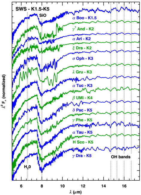
Figure 3.— SWS spectra of the K giants and supergiants showing oxygen-rich molecular absorption, plotted and labeled as in Figure 1. These spectra were processed and calibrated by Engelke et al. (2006).

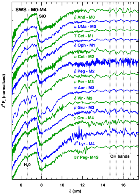
Figure 4.— SWS spectra of the early M giants (M0–M4), plotted and labeled as in Figure 1. These spectra are from Engelke et al. (2006).

Figure 3 shows the SWS spectra of the 12 K giants and one K supergiant in our comparison sample. The spectra show a SiO band which grows stronger with later spectral class. Three spectra, $\gamma^{1}$ And, $\lambda$ Gru, and $\pi$ Aur, are affected by artificial structure in the SiO band, but this has little impact on our measured equivalent width. H₂O absorption at 6.6 $\mu$m is not apparent in any of the spectra.

Table 2 notes that in 15 of the 26 SWS spectra calibrated by Engelke et al. (2006), the data past 12 $\mu$m are based on a template. The long-wavelength data in these spectra were too noisy and difficult to calibrate, leading Engelke et al. (2006) to replace them with the average of all 15, fitted to the photometry for each source. Therefore, while many of the spectra in Figure 3 show clear OH band structure, those data are not independent, and we cannot use them in our analysis. The same is true in Figure 4. Consequently, we will limit our spectral analysis of the SWS data to the SiO and H₂O bands and not consider the OH bands.

Figure 4 continues the SWS sequence to M4, showing the onset of H₂O absorption at spectral class M0 and the continued strengthening of the SiO band. Again, in most of the spectra, the OH bands are actually from a template spectrum.

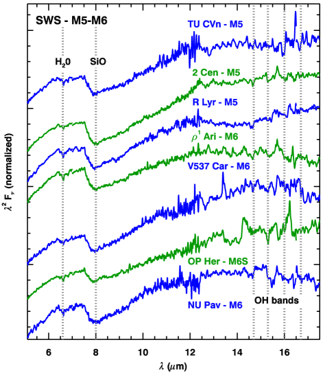
Figure 5.— SWS spectra of the late M giants (M5–M6), plotted and labeled as in Figure 1. These spectra are from Sloan et al. (2003b).

Figure 5 plots the seven spectra from the SWS not re-processed by Engelke et al. (2006). As a group, these spectra show more artifacts, especially at $\sim$11–12 and 14–18 $\mu$m. The spectra are also redder than the earlier-type sources, suggesting the presence of optically thin dust emission. The spectra of 2 Cen, R Lyr, $\rho^{1}$ Ari, and to a lesser degree NU Pav all have inflections at $\sim$11–12 $\mu$m, which are consistent with the presence of alumina dust.

Because Engelke et al. (2006) corrected the shape of the spectra and forced them to match the photometry, the overall shape of the continuum should be reasonably reliable in Figures 3 and 4. The general shapes of the spectra in Figure 5, however, are strongly affected by dust and may also be affected by uncorrected artifacts in the data.

3. Analysis

3.1. Measuring the SiO and H₂O bands

Paper I described the general procedure for measuring the strength of the SiO band at 8 $\mu$m. They simultaneously fitted an Engelke function (Engelke, 1992), a template SiO profile, and an interstellar extinction profile based on the local extinction spectrum of Chiar & Tielens (2006). The Engelke function mimics the effect of the H^- ion, which has an opacity that increases with wavelength, by decreasing the effective blackbody temperature to longer wavelengths. The template SiO profile is an average of the SiO band in several of the SWS spectra, as described in Paper I. The fitting method forces the Engelke function through the IRS data at $\sim$6.5–7.5 $\mu$m and $\sim$12 $\mu$m, and adjusts the temperature, the depth of the SiO band, and the interstellar extinction $A_{V}$ to minimize the $\chi^{2}$ error between the resulting spectrum and the data from 6.8 to 11.2 $\mu$m.

The M giant sample forced several modifications to the approach in Paper I. With the cooler M giants, changes to the stellar temperature and $A_{V}$ were largely degenerate, requiring an independent estimate of $A_{V}$. We used the three-dimensional extinction model of Drimmel et al. (2003, hereafter D03). Their software provides two extinctions, and we used the rescaled values. The input distances were based on the Hipparcos parallaxes (van Leeuwen, 2007). In the six cases where the D03 code did not provide an extinction, we used the extinctions for that line of sight by Schlafly & Finkbeiner (2011, hereafter SF11). In seven cases, the D03 extinctions exceeded the SF11 extinctions, but the latter should be an upper limit since they represent the total extinction along a given line of sight to an infinite distance. In those cases, we used SF11.

For the SWS sample, D03 provided $A_{V}$ estimates for 22 sources. For the remaining 11, we used $A_{K}$ estimates by Tabur et al. (2009), converting to $A_{V}$ using the extinction law calibrated by Rieke & Lebofsky (1985). In seven additional cases, we used the extinctions from Tabur et al. (2009) in place of the D03 values because they were larger than D03.

Most of the M giants observed by both the IRS and SWS exhibit absorption from water vapor at $\sim$6.7 $\mu$m. In some spectra, this absorption is more significant, taking a substantial notch out of the spectrum from $\sim$6.4 $\mu$m all the way to the beginning of the SiO band at 7.5 $\mu$m. These spectra required modifications to how we fitted the continuum. Instead of minimizing the $\chi^{2}$ error, we simply chose a temperature that forced an Engelke function fitted to the spectrum at $\sim$10.5–11 $\mu$m to pass through the spectrum somewhere between $\sim$6.3 and 7.5 $\mu$m. These wavelength ranges could vary from one spectrum to the next, depending on the strength of red wing of the SiO band, possible contamination from cool dust, and the strength and structure of the H₂O band.

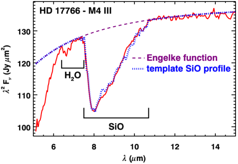
Figure 6.— To measure the equivalent width of the SiO and H₂O bands, we fit an Engelke function, assuming that the data past $\sim$11 $\mu$m and at least some of the data in the 6–7.5 $\mu$m range are from the continuum. The equivalent width is integrated underneath the continuum, assuming that the absorption from 6.4 to 7.5 $\mu$m is from H₂O and from 7.5 to 10.7 $\mu$m is from SiO.

Table 3SiO and H₂O equivalent widths in the IRS sample

Target	Parallax	$A_{V}$	$A_{V}$	Fitted	Eq. Width (SiO)	Eq. Width (H2O)
	(mas)	(mag)	Ref.	$T$ (K)	($\mu$m)	(nm)
HD 13570	1.3 $\pm$ 0.5	0.082	SF11	6350	0.194 $\pm$ 0.007	6.0 $\pm$ 3.0
HD 19554	2.9 $\pm$ 0.9	0.079	SF11	3300	0.264 $\pm$ 0.003	4.8 $\pm$ 3.2
HD 107893	1.4 $\pm$ 0.8	0.108	D03	10000	0.218 $\pm$ 0.006	5.9 $\pm$ 2.8
HD 17678	1.7 $\pm$ 1.3	0.062	SF11	3000	0.242 $\pm$ 0.003	11.6 $\pm$ 2.7
BD+47 2949	2.9 $\pm$ 0.6	0.202	D03	2950	0.238 $\pm$ 0.007	3.1 $\pm$ 5.7
HD 206503	1.1 $\pm$ 0.7	0.102	SF11	3400	0.254 $\pm$ 0.005	5.7 $\pm$ 3.0
HD 122755	1.7 $\pm$ 0.9	0.110	D03	2850	0.220 $\pm$ 0.004	31.6 $\pm$ 2.3
HD 177643	1.3 $\pm$ 0.9	0.181	D03	10000	0.345 $\pm$ 0.006	$-$13.1 $\pm$ 17.4
HD 189246	1.5 $\pm$ 1.0	0.221	SF11	3800	0.289 $\pm$ 0.007	5.5 $\pm$ 1.9
HD 26231	1.3 $\pm$ 0.7	0.025	SF11	2550	0.245 $\pm$ 0.003	32.1 $\pm$ 5.5
HD 127693	1.4 $\pm$ 1.1	0.233	D03	4850	0.292 $\pm$ 0.011	8.7 $\pm$ 2.3
HD 223306	2.5 $\pm$ 1.1	0.035	SF11	4300	0.259 $\pm$ 0.005	8.1 $\pm$ 3.1
HD 17766	1.8 $\pm$ 0.8	0.060	SF11	3400	0.306 $\pm$ 0.003	7.4 $\pm$ 3.4
HD 32832	$-$0.1 $\pm$ 0.7	0.048	SF11	2450	0.225 $\pm$ 0.006	21.0 $\pm$ 2.2
HD 46396	1.2 $\pm$ 0.6	0.150	SF11	3100	0.282 $\pm$ 0.006	6.9 $\pm$ 3.1
HD 68422	1.1 $\pm$ 0.9	0.381	D03	2850	0.281 $\pm$ 0.011	27.1 $\pm$ 5.3
HD 74584	3.3 $\pm$ 0.5	0.428	SF11	2750	0.291 $\pm$ 0.012	11.8 $\pm$ 3.8
HD 76386	1.8 $\pm$ 0.8	0.070	SF11	3000	0.273 $\pm$ 0.003	15.5 $\pm$ 4.2
HD 8680	4.5 $\pm$ 1.1	0.041	SF11	4200	0.259 $\pm$ 0.006	13.3 $\pm$ 3.8
BD+44 2199	$-$0.5 $\pm$ 1.1	0.031	D03	7950	0.323 $\pm$ 0.005	67.4 $\pm$ 2.6

Table 4SiO and H₂O equivalent widths in the SWS sample

Target	Parallax	$A_{V}$	$A_{V}$	Fitted	Eq. Width (SiO)	Eq. Width (H2O)
	(mas)	(mag)	Ref.	$T$ (K)	($\mu$m)	(nm)
$\alpha$ Boo	88.8 $\pm$ 0.5	0.002	D03	4950	0.147 $\pm$ 0.000	$\cdots$
$\gamma^{1}$ And	8.3 $\pm$ 1.0	0.034	D03	4000	0.188 $\pm$ 0.002	$\cdots$
$\alpha$ Ari	49.6 $\pm$ 0.2	0.027	D03	5250	0.102 $\pm$ 0.001	$\cdots$
$\xi$ Dra	29.0 $\pm$ 0.1	0.018	T09	4450	0.086 $\pm$ 0.001	$\cdots$
$\sigma$ Oph	3.6 $\pm$ 0.3	0.188	T09	3400	0.199 $\pm$ 0.007	$\cdots$
$\lambda$ Gru	13.5 $\pm$ 0.2	0.042	D03	4600	0.220 $\pm$ 0.003	$\cdots$
$\alpha$ Tuc	16.3 $\pm$ 0.6	0.083	D03	4900	0.164 $\pm$ 0.003	$\cdots$
$\beta$ UMi	24.9 $\pm$ 0.1	0.014	D03	3650	0.172 $\pm$ 0.000	$\cdots$
$\delta$ Psc	10.5 $\pm$ 0.2	0.080	T09	4500	0.208 $\pm$ 0.003	$\cdots$
$\gamma$ Phe	14.0 $\pm$ 0.3	0.033	D03	3750	0.239 $\pm$ 0.001	$\cdots$
$\alpha$ Tau	48.9 $\pm$ 0.8	0.063	T09	3850	0.267 $\pm$ 0.002	$\cdots$
H Sco	9.5 $\pm$ 0.2	0.143	T09	3400	0.289 $\pm$ 0.005	$\cdots$
$\gamma$ Dra	21.1 $\pm$ 0.1	0.018	T09	4250	0.211 $\pm$ 0.001	$\cdots$
$\beta$ And	16.5 $\pm$ 0.6	0.027	D03	4250	0.324 $\pm$ 0.000	19.5 $\pm$ 0.7
$\mu$ UMa	14.2 $\pm$ 0.5	0.009	T09	3600	0.302 $\pm$ 0.001	10.5 $\pm$ 0.7
7 Cet	7.3 $\pm$ 0.3	0.045	D03	3400	0.278 $\pm$ 0.001	8.3 $\pm$ 0.1
$\delta$ Oph	19.1 $\pm$ 0.2	0.098	T09	3600	0.266 $\pm$ 0.003	12.2 $\pm$ 0.2
$\alpha$ Cet	13.1 $\pm$ 0.4	0.107	T09	3500	0.320 $\pm$ 0.003	9.8 $\pm$ 0.1
$\beta$ Peg	16.6 $\pm$ 0.2	0.070	D03	2800	0.213 $\pm$ 0.000	23.8 $\pm$ 1.7
$\rho$ Per	10.6 $\pm$ 0.2	0.055	D03	3300	0.228 $\pm$ 0.003	35.8 $\pm$ 4.7
$\pi$ Aur	4.3 $\pm$ 0.6	0.125	T09	3800	0.348 $\pm$ 0.003	21.7 $\pm$ 0.8
$\delta$ Vir	16.4 $\pm$ 0.2	0.027	T09	3100	0.296 $\pm$ 0.001	11.8 $\pm$ 0.6
$\beta$ Gru	18.4 $\pm$ 0.4	0.009	T09	2950	0.293 $\pm$ 0.001	14.5 $\pm$ 1.1
$\gamma$ Cru	36.8 $\pm$ 0.2	0.045	T09	2850	0.308 $\pm$ 0.000	14.1 $\pm$ 1.1
$\delta^{2}$ Lyr	4.4 $\pm$ 0.2	0.098	D03	2200	0.424 $\pm$ 0.002	20.9 $\pm$ 5.1
57 Peg	4.2 $\pm$ 0.3	0.089	T09	4350	0.272 $\pm$ 0.001	13.4 $\pm$ 2.3
TU CVn	4.7 $\pm$ 0.3	0.047	D03	2150	0.393 $\pm$ 0.003	40.9 $\pm$ 4.2
2 Cen	17.8 $\pm$ 0.2	0.114	D03	2250	0.391 $\pm$ 0.001	21.3 $\pm$ 0.6
R Lyr	10.9 $\pm$ 0.1	0.036	T09	2100	0.361 $\pm$ 0.002	34.2 $\pm$ 1.4
$\rho^{1}$ Ari	9.3 $\pm$ 0.3	0.304	T09	2400	0.342 $\pm$ 0.006	25.2 $\pm$ 3.2
V537 Car	3.0 $\pm$ 0.5	0.214	T09	1300	0.369 $\pm$ 0.002	45.7 $\pm$ 1.8
OP Her	3.4 $\pm$ 0.3	0.129	D03	1450	0.238 $\pm$ 0.001	14.0 $\pm$ 0.5
NU Pav	6.9 $\pm$ 0.3	0.073	D03	1800	0.345 $\pm$ 0.002	48.0 $\pm$ 2.8

We then integrated the SiO absorption from 7.5 $\mu$m to 10.7 $\mu$m, accounting for the interstellar extinction profile based on our estimated $A_{V}$. For the K giant sample, Paper I measured the SiO band strength from 7.3 $\mu$m, but in the M giants, H₂O absorption at 7.3 $\mu$m forced us to shift to 7.5 $\mu$m. Figure 6 illustrates the technique for a sample spectrum.

To estimate the uncertainties arising from our estimates of $A_{V}$, we measured the SiO and H₂O equivalent widths with $A_{V}$ set to zero. We replaced the uncertainty in equivalent width with the difference between the two measurements if the difference was larger. Tables 3 and 4 give the results for the IRS and SWS samples, respectively. Because of the effect of pointing on the overall shape of the spectrum (Section 2.1), the fitted temperatures in Table 3 are not physically meaningful. They are better interpreted as a guide to the photometric accuracy of the spectrum in question. We capped the temperature at 10⁴ K for HD 107893 and HD 177643, which appear to be the most strongly affected by pointing. The fitted temperatures in Table 4 are more reasonable, if still of limited accuracy, due primarily to the method used to conform the SWS spectra to the photometry by Engelke et al. (2006). The low apparent temperatures of the last seven M giants in Table 4 may be indicating the presence of dust.

Paper I found that the $B-V$ color tracked the equivalent width of the SiO band better than spectral class for the K giants. However, the behavior of $B-V$ versus spectral class is not monotonic for the M giants, as explained in Appendix 1. Consequently, we will focus primarily on the behavior of the SiO, H₂O, and OH bands as a function of spectral class in this paper.

3.2. Silicon monoxide

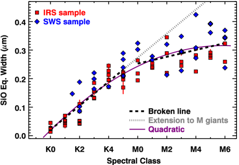
Figure 7.— Equivalent width of the SiO band as a function of spectral class. The strength of the SiO band increases rapidly from K0 to K5, then more slowly from M0 to M6, with considerable scatter at each spectral class. In most cases, the uncertainties are smaller than the plotting symbols. The figure includes lines fitted separately to the K giants and M giants (dashed line), with the K-giant line extended to later spectral classes (dotted line). A quadratic function (solid purple line) also follows the observed data about as well as the broken linear fit.

Figure 7 shows how the strength of the fundamental SiO band at 8 $\mu$m depends on spectral class for the full IRS sample of K and M giants and the SWS sample. Paper I fit a quadratic to the relation for just the IRS-observed K giants and the result was close to linear. Here, we fit a line to the K giants (dashed line from K0 to K5). Extending that line to later spectral classes (dotted line) clearly overpredicts the actual observed SiO equivalent widths for the M giants.

The slope of the line for the K giants is 0.042 $\mu$m per spectral class, while if we fit a separate line to spectral classes M0–M6, the slope is only 0.012 $\mu$m per class. Concentrating on just the IRS sample, the standard deviation in equivalent width increases from $\sim$0.02 $\mu$m for the K giants to over $\sim$0.03 $\mu$m in the M giants. Thus the change in SiO strength from one spectral class to the next is larger than the scatter in the K giants, but smaller in the M giants.

There is nothing unique about our choice to fit a broken line to the data, with the break between K5 and M0. As long as the break is between K2/K3 and M0/M1, the $\chi^{2}$ residuals are about the same. A quadratic (shown as a purple curve in Figure 7) also works about as well. Whatever the nature of the specific relationship, the IRS spectra show that as the stars grow cooler, the equivalent width of the SiO absorption band at 8 $\mu$m increases more slowly with spectral class. In addition, the spread in SiO band strength is considerable in most spectral classes (from K2 on), and for the coolest giants in our sample, the spread is considerably larger than the increase in band strength from one subclass to the next.

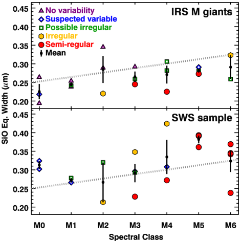
Figure 8.— Equivalent width of the SiO band for the M giants, color-coded by variability. The dotted line is fitted to all of the plotted data and is the same in both panels. The error bars for the mean equivalent widths are the standard deviations at each spectral class. No dependence on variability is apparent.

Figure 8 concentrates on just the M giants and color codes them by their variability class. The IRS and SWS spectra show no evidence that more variable stars are associated with deeper SiO absorption bands. The dotted line in both panels is the same line fitted to the 40 M giants observed by the IRS and SWS in Figure 7. To compare the SiO band depth versus variability, we have grouped our sample into the more variable stars, which includes the 17 stars classified as irregulars or semi-regulars. The other 23 stars classified as possible irregulars, suspected variables, or with no identified variability are the control sample. For each group, we measure the mean difference in actual equivalent width versus the equivalent width expected from the fitted line for that spectral class. The control sample has a mean difference of $-$1.0 nm, compared to an uncertainty in the mean of 7.4 nm. The more variable stars have a mean difference of 0.8 $\pm$ 15.4 nm. Thus we can conclude that variability has virtually no impact on SiO equivalent width.

3.3. Water vapor

Most previous studies of emission or absorption from water vapor in the spectra of evolved stars have been of discrete lines, either in the vicinity of 6.5–6.7 $\mu$m (e.g. Tsuji et al., 1997; Tsuji, 2001) or in the 12 $\mu$m region (e.g. Ryde et al., 2002, 2006). However, some of the spectra in our sample of M giants show decidedly more absorption, most notably BD+44 2199 in Figure 2, where the absorption is strong enough from 6.4 to 7.5 $\mu$m to leave what looks like an apparent emission feature at 6.2–6.3 $\mu$m.

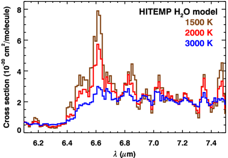
Figure 9.— The absorption cross section of H₂O at three temperatures. These synthetic spectra are based on the Kspectrum code and the HITEMP database (Rothman et al., 2010), and they have been downsampled to a resolution about twice that of the IRS at these wavelengths. As the temperature drops, the bands at $\sim$6.6 and 6.8 $\mu$m grow more prominent.

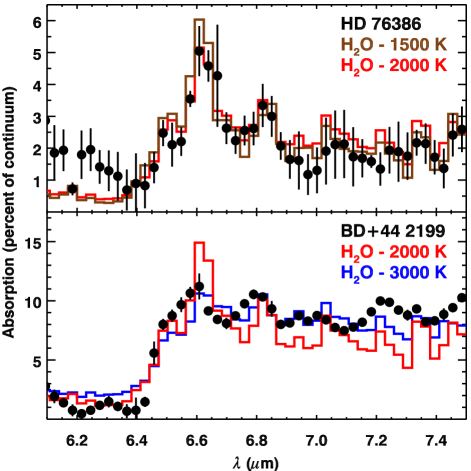
Figure 10.— Spectra of the absorption in two spectra in our sample compared to the synthetic water vapor absorption in Fig. 9. Top: BD+44 2199 has the strongest H₂O absorption in our sample, and the minimal substructure at $\sim$6.6 and 6.8 $\mu$m is most consistent with our synthetic spectrum at 3000 K, which is roughly the dissociation temperature of H₂O. Bottom: HD 76386 is an example of the several spectra which show two apparent absorption bands from H₂O at $\sim$6.6 and 6.8 $\mu$m, and these are generally more consistent with cooler temperatures.

Figure 9 presents synthetic spectra of H₂O generated with the line lists from the HITEMP database (Rothman et al., 2010) and the Kspectrum software package (Wordsworth et al., 2010). HITEMP includes over 100 million water vapor lines and is more suitable for warm stellar atmospheres than databases such as HITRAN, which is designed for the Earth’s atmosphere (Rothman et al., 2012). Kspectrum generates high-resolution spectra from line-by-line databases using Voigt and Lorentz line profiles without applying radiative transfer methods. It has been used primarily to generate synthetic spectra from planetary atmospheres (e.g. Ramirez et al., 2014), and we use it to generate cross sections as a function of wavelength and temperature. We found that pressure had little effect. As the temperature of water vapor drops from 3000 K (roughly its dissociation temperature) to 2000 K, the absorption structure in the 6–8 $\mu$m region develops two prominent bands at $\sim$6.6 and 6.8 $\mu$m.

Figure 10 compares the absorption structure in two of our spectra to the synthetic H₂O spectra and demonstrates that the structure in the IRS spectra at 6–7 $\mu$m is indeed from water vapor. BD+44 2199 shows the strongest H₂O absorption in our sample, and resembles most closely the synthetic spectrum at 3000 K, because it doesn’t show a prominent 6.6 $\mu$m feature. The deep absorption in the observed spectrum requires a higher column density than the other spectra. Many of the spectra with weaker water vapor absorption show two distinct bands at $\sim$6.6 and 6.8 $\mu$m, which the cooler synthetic spectra fit well. HD 76386 is a typical example, and the 2000 K model fits its spectrum better than the 1500 K model.

The synthetic spectra firmly identify water vapor as the carrier of the excess absorption between 6.4 and 7.5 $\mu$m in the M giants. The spectra also show that varying the temperature of the water vapor can explain the different structures apparent in the 6–7 $\mu$m range in our sample. These preliminary modeling results point to the potential for more detailed analysis, but that is beyond the scope of the present paper.

Figure 9 shows that the absorption from H₂O does not go to zero in the 6.2–6.3 $\mu$m region. Nor does it go to zero at 7.5 $\mu$m at the edge of the SiO band. Thus our measurement from 6.4–7.5 $\mu$m is only a partial measure of the H₂O absorption and should be treated somewhat qualitatively.

The water vapor also affects our continuum fitting, but its impact on the measured SiO equivalent width is small. Our fitting of an Engelke function to the continuum will still effectively isolate the SiO band even if water vapor absorption shifts the entire continuum downward. and should still lead to a reliable measurement.

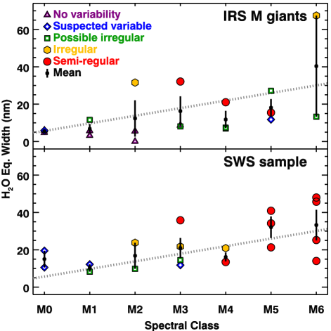
Figure 11.— H₂O absorption in the M giants, color-coded by variability. As in Fig. 8, the dotted line is the same in both panels, and the error bars for the means at each spectral class depict the standard deviations. The more variable stars tend to have the stronger H₂O bands.

A comparison of Figures 3 and 4 show that the H₂O absorption is not visible in the SWS targets of spectral class K. Thus we only consider the equivalent widths for H₂O measured for the M giants. Figure 11 plots the equivalent width as a function of spectral class for the M giants in both the IRS and SWS samples. The dotted line in both panels is fitted to all of the data, and it shows a gentle rise, 4.1 nm per spectral class, compared to a median standard deviation in each class of 4.6 nm for the IRS sample and 5.4 nm for the SWS sample. While the spread is substantial compared to the slope, the net change in absorption strength from M0 to M6 is 25 nm, or roughly five times the typical scatter.

Figure 11 shows that variable stars tend to have stronger H₂O bands. The IRS sample includes a range of variabilities from M2 to M6, and in four of the five cases, the more variable stars have stronger H₂O contributions. In the SWS sample, only M2–M4 show a distribution of variabilities, and in two of the three cases, the same result holds.

To be more rigorous, we can apply the same test used for the effect of variability on the SiO band and compare the mean difference from the fitted line for the 17 irregulars and semi-regulars to the 23 other less variable stars. The first group has a mean difference of $+$6.5 $\pm$ 3.3 nm, while the second is $-$5.4 $\pm$ 1.8 nm. Thus the more variable stars have equivalent widths typically 11.9 nm stronger than the less variable stars. The combined uncertainty in this difference is 3.8 nm, making the difference between the two variability groups a 3.2-$\sigma$ result.

3.4. Hydroxyl

The OH bands are faint, typically only 1–2% of the continuum and requiring signal/noise ratios (SNRs) well over 100 for a reasonable detection. Consequently Paper I limited their analysis of the OH bands in the K giants to the five standards observed repeatedly over the cryogenic Spitzer mission and five signifiantly brighter K giants observed for cross-calibration purposes. These ten stars revealed a strong dependence of OH band strength with spectral class in the K giants, as measured in the four bands between 14 and 17 $\mu$m.

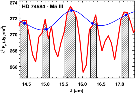
Figure 12.— Extracting the OH absorption bands between 14.5 and 17.1 $\mu$m. The continuum (blue) is estimated with a spline, using the data in the shaded regions. The data between the shaded regions are the OH absorption bands. The strongest OH band in this spectrum (at 16 $\mu$m), is only $\sim$2% of the continuum.

Table 5OH equivalent widths in the IRS M giants

Target	Eq. width
	14–17 $\mu$m (nm)
HD 13570	13.5 $\pm$ 3.0
HD 19554	18.6 $\pm$ 1.9
HD 107893	16.1 $\pm$ 3.9
HD 17678	21.6 $\pm$ 4.0
BD+47 2949	13.2 $\pm$ 2.3
HD 206503	21.1 $\pm$ 3.6
HD 122755	9.1 $\pm$ 3.0
HD 177643	18.2 $\pm$ 2.3
HD 189246	15.0 $\pm$ 3.0
HD 26231	21.4 $\pm$ 2.3
HD 127693	20.3 $\pm$ 2.5
HD 223306	9.5 $\pm$ 2.5
HD 17766	11.0 $\pm$ 2.8
HD 32832	12.8 $\pm$ 2.4
HD 46396	17.5 $\pm$ 2.3
HD 68422	18.1 $\pm$ 2.2
HD 74584	20.3 $\pm$ 2.3
HD 76386	19.1 $\pm$ 3.7
HD 8680	17.9 $\pm$ 3.5
BD+44 2199	22.6 $\pm$ 5.2

Our single pointings at the 20 M giants had SNRs just sufficient enough to detect the OH bands. We used the same approach as Paper I to maintain consistency, determining the continuum in the intervals between the bands and then fitting a spline through the estimated continua. Figure 12 illustrates the process. The example chosen, HD 74584, is one of the better-behaved spectra in this spectral region. We tried several alternative approaches, such as coadding the spectra at each spectral class or forcing the spline continuum points to align with a Rayleigh-Jeans tail, with no improvement in the results. Table 5 presents the measured equivalent widths, summed from the four bands in the 14–17 $\mu$m region.

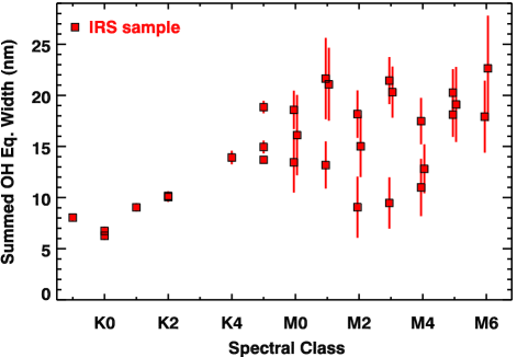
Figure 13.— OH band strength summed from 14.5 to 17.1 $\mu$m and plotted as a function of spectral class for the sources observed with the IRS. The OH bands grow stronger from K0 to K5 and then plateau to later spectral classes. The M giants have been slightly offset horizontally to limit the overlap of the error bars.

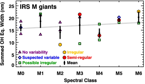
Figure 14.— Equivalent width of the OH bands for the M giants, color-coded by variability. The dotted line is fitted to just the data plotted in this panel and shows the lack of a strong dependence on spectral class in the M giants. Variability does not appear to be a factor, either. The error bars for the mean equivalent widths give the standard deviations.

Figure 13 shows the result of our extractions: considerable scatter in each spectral class from M0 to M6, with a median standard deviation of 2.4 nm. The line fitted to the M giants observed by the IRS has a slope of only 0.4 nm per spectral class, making the apparent change in band strength from M0 to M6 comparable to the typical scatter in each spectral class. The IRS spectra do not reveal any significant dependence of equivalent width on spectral class for the M giants. Figure 14 shows that variability is not responsible for the scatter in OH band strength. For both the five variables and the 15 stars in the control sample, the mean difference between actual equivalent widths and those expected from the fitted line are statistically insignificant ($\sim$0.1 $\sigma$).

4. Discussion

4.1. SiO and OH absorption

Section 3.2 showed that the equivalent width of the fundamental SiO band at 8 $\mu$m generally increased toward later spectral classes, but with considerable scatter and a decrease in the slope with later spectral class. Heras et al. (2002) previously noted each of these points, and thus our results fully confirm theirs. Because we have more carefully constrained the IRS sample by luminosity class, we can conclude that the scatter is not due to luminosity. Nor is it due to variability. Paper I suggested that metallicity could possibly influence the equivalent width of the SiO band and produce the observed scatter in a given spectral class. While that hypothesis is still plausible, for both K and M giants, it remains untested.

We have detected OH bands in all of the M giants observed with the IRS, and while the OH band strength increases with later spectral types in the K giants, the dependence is much flatter in the M giants and shows substantial scatter. We have detected no effect of stellar variability on OH band strength. While we were able to detect OH absorption bands in all 20 of the M giants observed by the IRS, the spectra are right at the threshold for useful analysis. Higher quality data, with better resolutions and SNRs, would help substantially in our understanding of how the OH bands behave and depend on stellar properties.

4.2. H₂O absorption

Previous identifications of H₂O in the 6–7 $\mu$m region were based on individual lines in higher-resolution data (e.g. Tsuji et al., 1997; Tsuji, 2001). Our synthetic spectra show that H₂O is responsible for the broad absorption structure apparent in most of our M-giant spectra from 6.3 $\mu$m to the SiO bandhead at 7.5 $\mu$m.

The synthetic spectra demonstrate that the HITEMP line list is complete enough to support efforts to model the spectra in this wavelength regime, although some discrepancies between the observations and the synthetic spectra are still apparent, especially to the red of $\sim$7 $\mu$m. For example, both panels of Figure 10 show an absorption feature at 7.1 $\mu$m in the synthetic spectra which is not apparent in the observed data.

Our limited modeling effort suggests that the different spectral structures seen in the 6.4–6.8 $\mu$m region can be explained by different temperatures. In the example presented in Figure 10, BD+44 2199 requires a higher column density and warmer temperatures compared to HD 76386. Figure 9 shows that the relative strengths of the 6.6 and 6.8 $\mu$m bands might serve as a temperature diagnostic. In addition, the position of the 6.8 $\mu$m band appears to shift to the red with cooler temperatures. Further modeling is required to substantiate these tentative conclusions.

Stars which are more variable tend to have stronger absorption from H₂O in the 6.3–7.5 $\mu$m range. Thus stellar variability plays a role in the formation of H₂O, but not OH or SiO.

The IRS and SWS data show a gentle but measurable increase in H₂O band strength with spectral class in the M giants. This result differs from the previous conclusion of Ardila et al. (2010), who found no apparent change in band strength with spectral class, but it should be kept in mind that they examined a smaller number of M giants than the current sample, and the stars in their sample tended to be relatively non-variable.

Tsuji (2000) detected water vapor emission in the spectrum of the supergiant $\mu$ Cep and proposed that it arose from an extended molecular sphere, which he identified as a MOLsphere. Tsuji (2001) added several red giants to the list of possible MOLsphere sources, but the idea remains controversial. High-resolution spectra of $\alpha$ Boo in the 11–12 $\mu$m range show absorption lines with temperatures more consistent with the photosphere of the star than a detached molecular layer (Ryde et al., 2002). This star is much warmer than the typical H₂O absorber in our samples, but Ryde et al. (2006) found a similar result at $\sim$12 $\mu$m in $\mu$ Cep, which has a spectral type of M1–2 Ia–Iab. Further high-resolution spectra show similar results for a larger sample of K and M giants (Ryde et al., 2015), with generally stronger absorption than expected and temperatures consistent with a cool photosphere.

For geometric reasons, water vapor in an extended molecular sphere should produce emission lines, or at a minimum substantially weakened absorption lines. Tsuji (2009) modified his original MOLsphere hypothesis to account for this lack of emission lines by suggesting that the molecules may exist in clouds in the outer atmospheres of the stars. In our sample of 20 M giants observed by the IRS and 20 observed by the SWS, not one shows water vapor in emission. That result places some limits on the patchiness of the clouds and how far above the photosphere they could lie.

4.3. Considering the photometry

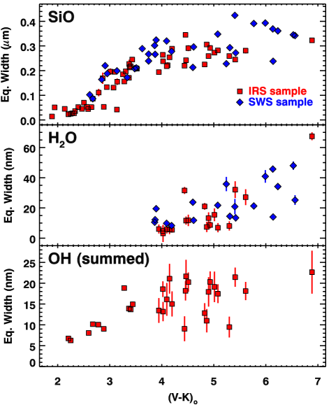
Figure 15.— The equivalent width of the SiO band, measured H₂O, and summed OH bands as a function of dereddened $V-K$ color for the IRS and SWS samples.

Figure 15 plots the equivalent widths of the infrared molecular bands versus $(V-K)_{0}$. Appendix 1 explains how we determined the photometric colors for our sample and shows that $B-V$, which Paper I found to be a useful diagnostic for K giants, is double-valued in M giants. The $V-K$ color reddens monotonically with spectral class and can give us more insight on the behavior of the molecular bands.

For SiO as a function of $V-K$ color, the change in slope between the K and M giants is apparent, just as when plotting versus spectral class. In Figure 7, a fair fraction of the SWS sources were above the line segments fitted to the combined sample, but in the top panel of Figure 15, these sources have moved closer to the rest of the population. At the red end of the sample, six out of the seven SWS sources at M4–M6 with strong SiO absorption (equivalent width $>$ 0.34 $\mu$m), have the reddest $V-K$ colors in the sample. Only BD+44 2199 in the IRS sample is redder. Plotting versus color instead of spectral class aligns these sources better with the trends shown by the rest of the sample.

4.4. Towards dust production

The SWS sample represents a sizable subset of the red giants closest to the Sun, and it shows how the percentage of variables increases quickly past a spectral class of M2. All of the SWS sources of spectral class M4–M6 are irregulars or semi-regulars. When selecting the IRS sample, we tried to avoid known variables, but we were unable to keep them out of the sample altogether. Irregular and semi-regular variables are long-period variables typically associated with the thermally pulsing asymptotic giant branch (AGB), and their presence in our sample reveals that we are looking at two groups of stars. AGB stars appear to dominate spectral classes past M4. Earlier spectral classes could be either making their first ascent of the red-giant branch (RGB) or are early AGB stars.

The likely presence of dust in several of the reddest sources in our sample also suggests that it includes AGB stars beginning the mass-loss process. As previously noted, several of the reddest sources show inflections in their spectra suggestive of alumina dust. BD+44 2199 has the reddest $V-K$ color in the sample, the strongest H₂O absorption, the second strongest SiO absorption, and its spectrum shows an increasing excess with wavelength to the red of 10 $\mu$m. Both its $V-K$ color and its mid-infrared spectrum indicate that it is producing dust. The reddest sources in the SWS sample account for most of the remaining strong SiO and H₂O absorbers. These are also likely to be thermally pulsing AGB stars beginning to lose mass and produce dust.

Our spectra reveal the molecular precursors to the dust we expect to form as these stars continue to evolve, and they point to the potential for further observations. Deeper integrations and higher spectral resolutions would reveal in more detail the physical conditions of the OH and H₂O molecules and better constrain their physical locations in the stellar atmospheres. In particular, the H₂O bands at these wavelengths look to have strong diagnostic possibilities. New samples in systems with known distances and metallicities may be the best means of investigating the origin of the scatter in the present sample.

5. Summary

We have observed 20 M giants with the IRS on Spitzer. These spectra, combined with our previous IRS sample of 33 K giants and the SWS sample of 13 K-type stars and 20 M giants, reveal how the strength of the SiO, OH, and H₂O bands depend on spectral class and $V-K$ color.

The equivalent width of the SiO band at 8 $\mu$m increases as the stars grow cooler, but it increases more gradually at later spectral classes. The scatter is considerable and intrinsic to the sample. These results confirm the earlier study by Heras et al. (2002). The scatter does not result from differences in the luminosities or variability properties of the stars.

Our synthetic spectra confirm that the structure in our spectra between 6.3 and 7.5 $\mu$m is from H₂O absorption. These bands are not easily detected in the K giants, but in the M giants, they increase in strength as the stars grow cooler, but again, with considerable scatter. In this case, the scatter arises from the variability properties of the stars, with more variable sources generally showing stronger absorption in a given spectral class.

The OH bands at 14–17 $\mu$m climb in strength from K0 to K5, but for cooler stars show little obvious dependence on temperature. The scatter in equivalent widths in the M giants is considerable. Variability plays no obvious role on OH band strength.

Appendix 1. Photometry

Paper I found that the $B-V$ color of the K giants in their sample tracked the equivalent width of the SiO band at 8 $\mu$m somewhat better than the spectral class. They proposed modifying some of the spectroscopically assigned spectral classifications on this basis. It follows that we should investigate the photometric properties of the SWS sample and the M giants observed by the IRS.

Table 6Photometry for the SWS sample

Target	$B$	$V$	Optical	$B_{T}$	$V_{T}$	$J$	$H$	$K$	Near-IR
	(mag)	(mag)	Reference	(mag)	(mag)	(mag)	(mag)	(mag)	Reference
$\alpha$ Boo	1.18	$-$0.05	J66, L70	$\cdots$	0.161 $\pm$ 0.014	$-$2.229 $\pm$ 0.100	$-$2.938 $\pm$ 0.078	$-$2.961 $\pm$ 0.212	CIO
$\gamma^{1}$ And	3.63	2.26	L71	3.984 $\pm$ 0.014	2.308 $\pm$ 0.009	$-$0.030 $\pm$ 0.079	$-$0.715 $\pm$ 0.021	$-$0.840 $\pm$ 0.048	CIO
$\alpha$ Ari	3.15	2.00	J66, L70	3.487 $\pm$ 0.014	2.125 $\pm$ 0.009	0.098 $\pm$ 0.136	$-$0.529 $\pm$ 0.036	$-$0.634 $\pm$ 0.039	CIO
$\xi$ Dra	4.93	3.75	J66	5.253 $\pm$ 0.014	3.853 $\pm$ 0.009	1.767 $\pm$ 0.022	1.192 $\pm$  $\cdots$	1.038 $\pm$ 0.029	CIO
$\sigma$ Oph	5.83	4.33	J66	6.293 $\pm$ 0.014	4.496 $\pm$ 0.009	1.815 $\pm$ 0.092	1.100 $\pm$  $\cdots$	1.003 $\pm$ 0.015	CIO
$\lambda$ Gru	5.83	4.46	J66	6.270 $\pm$ 0.014	4.618 $\pm$ 0.009	2.264 $\pm$ 0.030	1.436 $\pm$ 0.248	1.506 $\pm$ 0.027	P10, 2MASS
$\alpha$ Tuc	4.25	2.86	J66	4.679 $\pm$ 0.014	2.998 $\pm$ 0.009	0.558 $\pm$  $\cdots$	$-$0.080 $\pm$  $\cdots$	$-$0.090 $\pm$  $\cdots$	CIO
$\beta$ UMi	3.55	2.08	J66	3.998 $\pm$ 0.014	2.215 $\pm$ 0.009	$-$0.450 $\pm$  $\cdots$	$\cdots$	$-$1.315 $\pm$ 0.106	CIO
$\delta$ Psc	5.95	4.44	J66	6.399 $\pm$ 0.015	4.594 $\pm$ 0.009	1.777 $\pm$ 0.056	1.000 $\pm$ 0.028	0.857 $\pm$ 0.049	CIO
$\gamma$ Phe	4.98	3.41	J66	5.496 $\pm$ 0.014	3.613 $\pm$ 0.009	0.542 $\pm$ 0.013	$\cdots$	$-$0.360 $\pm$ 0.010	P10
$\alpha$ Tau	2.40	0.86	L70	2.937 $\pm$ 0.006	1.160 $\pm$ 0.011	$-$1.887 $\pm$ 0.067	$-$2.628 $\pm$ 0.100	$-$2.825 $\pm$ 0.198	CIO
H Sco	5.73	4.16	J66	6.238 $\pm$ 0.015	4.346 $\pm$ 0.009	1.326 $\pm$ 0.021	$\cdots$	0.394 $\pm$ 0.018	P10
$\gamma$ Dra	3.74	2.22	J66	4.246 $\pm$ 0.014	2.381 $\pm$ 0.009	$-$0.443 $\pm$ 0.043	$-$1.160 $\pm$  $\cdots$	$-$1.340 $\pm$ 0.065	CIO
$\beta$ And	3.62	2.05	J66, L70	4.155 $\pm$ 0.014	2.244 $\pm$ 0.009	$-$0.869 $\pm$ 0.078	$-$1.667 $\pm$ 0.067	$-$1.873 $\pm$ 0.074	CIO
$\mu$ UMa	4.64	3.05	J66	5.126 $\pm$ 0.014	3.216 $\pm$ 0.009	0.101 $\pm$ 0.012	$-$0.685 $\pm$ 0.006	$-$0.856 $\pm$ 0.043	CIO
7 Cet	6.12	4.46	J66	6.593 $\pm$ 0.015	4.629 $\pm$ 0.009	1.298 $\pm$  $\cdots$	0.369 $\pm$  $\cdots$	0.191 $\pm$  $\cdots$	CIO
$\delta$ Oph	4.34	2.75	J66	4.808 $\pm$ 0.014	2.896 $\pm$ 0.009	$-$0.241 $\pm$ 0.052	$-$1.030 $\pm$ 0.049	$-$1.266 $\pm$ 0.058	CIO
$\alpha$ Cet	4.17	2.53	L70	4.687 $\pm$ 0.014	2.716 $\pm$ 0.009	$-$0.629 $\pm$ 0.075	$-$1.462 $\pm$ 0.156	$-$1.683 $\pm$ 0.058	CIO
$\beta$ Peg	4.15	2.50	L70	4.610 $\pm$ 0.014	2.654 $\pm$ 0.009	$-$1.120 $\pm$ 0.065	$-$1.997 $\pm$ 0.066	$-$2.214 $\pm$ 0.067	CIO
$\rho$ Per	5.04	3.39	J66	5.372 $\pm$ 0.014	3.539 $\pm$ 0.009	$-$0.792 $\pm$ 0.073	$-$1.760 $\pm$  $\cdots$	$-$1.940 $\pm$ 0.035	CIO
$\pi$ Aur	5.97	4.25	J66	6.484 $\pm$ 0.014	4.516 $\pm$ 0.009	0.268 $\pm$ 0.039	$-$0.610 $\pm$  $\cdots$	$-$0.882 $\pm$ 0.054	CIO
$\delta$ Vir	4.97	3.38	J66, L70	5.382 $\pm$ 0.014	3.577 $\pm$ 0.009	$-$0.203 $\pm$ 0.070	$-$1.058 $\pm$ 0.049	$-$1.244 $\pm$ 0.048	CIO
$\beta$ Gru	3.73	2.11	J66	4.131 $\pm$ 0.014	2.287 $\pm$ 0.009	$-$2.126 $\pm$ 0.016	$-$3.120 $\pm$  $\cdots$	$-$3.220 $\pm$  $\cdots$	P10, CIO
$\gamma$ Cru	3.22	1.63	J66	$\cdots$	$\cdots$	$-$2.145 $\pm$ 0.205	$-$2.880 $\pm$ 0.200	$-$3.123 $\pm$ 0.088	CIO
$\delta^{2}$ Lyr	5.97	4.30	J66	6.302 $\pm$ 0.014	4.464 $\pm$ 0.009	$-$0.056 $\pm$ 0.043	$-$0.913 $\pm$ 0.110	$-$1.219 $\pm$ 0.042	CIO
57 Peg	6.58	5.11	J66	6.886 $\pm$ 0.015	5.294 $\pm$ 0.009	0.785 $\pm$ 0.007	$-$0.055 $\pm$ 0.092	$-$0.360 $\pm$ 0.085	CIO
TU CVn	7.39	5.84	N78	7.730 $\pm$ 0.015	6.022 $\pm$ 0.009	0.975 $\pm$ 0.021	0.090 $\pm$  $\cdots$	$-$0.180 $\pm$ 0.062	CIO
2 Cen	5.69	4.19	J66	6.023 $\pm$ 0.014	4.416 $\pm$ 0.009	$-$0.490 $\pm$ 0.021	$-$1.398 $\pm$ 0.077	$-$1.611 $\pm$ 0.138	CIO
R Lyr	5.59	4.00	J66	5.998 $\pm$ 0.014	4.355 $\pm$ 0.009	$-$0.922 $\pm$ 0.047	$-$1.803 $\pm$ 0.008	$-$2.069 $\pm$ 0.045	CIO
$\rho^{1}$ Ari	7.44	5.93	L70	7.416 $\pm$ 0.015	5.951 $\pm$ 0.010	0.218 $\pm$ 0.074	$-$0.735 $\pm$ 0.047	$-$1.020 $\pm$ 0.027	CIO
V537 Car	$\cdots$	$\cdots$	$\cdots$	8.429 $\pm$ 0.016	6.847 $\pm$ 0.010	1.410 $\pm$ 0.020	0.280 $\pm$ 0.306	0.368 $\pm$ 0.016	P10, 2MASS
OP Her	7.93	6.32	L70	8.211 $\pm$ 0.016	6.506 $\pm$ 0.010	1.240 $\pm$ 0.042	0.355 $\pm$ 0.024	0.080 $\pm$ 0.054	CIO
NU Pav	6.66	5.13	H70, N78	6.815 $\pm$ 0.015	5.235 $\pm$ 0.009	$-$0.250 $\pm$ 0.028	$-$1.220 $\pm$ 0.071	$-$1.510 $\pm$ 0.014	CIO

We used a similar procedure to that applied to the K giants, starting with Tycho magnitudes (Høg et al., 2000), then converting to colors and magnitudes in the Johnson system. Paper I used data from Bessell (2000) to determine the following conversion:

$$(B-V)_{0}=0.099+0.779(B_{T}-V_{T})_{0},$$ (1)

for 1.1 $\leq$ $B_{T}-V_{T}$ $\leq$ 1.9. However, most of our M giants are beyond the red limit. We can use the SWS sample to check the relation between Tycho and Johnson colors for the M giants. Table 6 gives $B$ and $V$ magnitudes in both the Johnson and Tycho systems for the SWS sample. These sources are bright enough that the Johnson magnitudes are from the seminal paper on the subject (Johnson et al., 1966)!

Table 6 also includes $JHK$ magnitudes, but here the brightness of the sources makes the task more difficult, because all of the sources are saturated in the 2MASS survey. To avoid the inaccuracies of the corrections for saturation, we have turned to the Catalog of Infrared Observations (CIO, version 5.1; Gezari et al., 2000). When the CIO provides multiple entries in a given filter, we determine the mean and standard deviation after rejecting outliers from the sample. We have not made a distinction between different filter sets, for example just reporting $K$ magnitudes intead of the usual 2MASS $K_{s}$. When the CIO does not provide photometry, we turned to the recalibration of bright sources observed by the Diffuse Infrared Background Experiment (DIRBE) on the Cosmic Background Explorer (COBE) by Price et al. (2010). We have treated DIRBE bands 1 and 2 as roughly equivalent to $J$ and $K$.

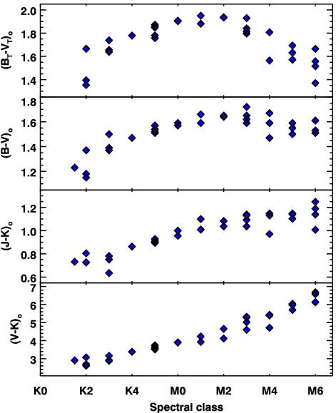
Figure 16.— Optical and near-infrared colors as a function of spectral class for the SWS sample, for which we have reliable photometry for all of the colors plotted.

Figure 16 plots $(B_{T}-V_{T})_{0}$, $(B-V)_{0}$, $(J-K)_{0}$, and $(V-K)_{0}$ versus spectral class. All of the colors have been dereddened using the $A_{V}$ estimates in Table 4 and the extinctions of Rieke & Lebofsky (1985), interpolating for the wavelengths of $B_{T}$ and $V_{T}$. Both $(B_{T}-V_{T})_{0}$ and $(B-V)_{0}$ reach a maximum at $\sim$M2, then decrease for later spectral classes. After the turnover, their slopes differ, with $(B_{T}-V_{T})_{0}$ falling more steeply than $(B-V)_{0}$.

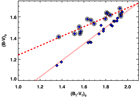
Figure 17.— Converting from $(B_{T}-V_{T})_{0}$ to $(B-V)_{0}$. Two conversions are required because later-type stars follow a different sequence. The dotted line is from Paper I and applies to the K giants. The dashed line is fitted to all stars of spectral class M2 or later (which are circled).

As a result, the conversion from $(B_{T}-V_{T})_{0}$ to $(B-V)_{0}$ is double-valued, as Figure 17 shows. Spectral classes up to and including M1 follow the relation from Paper I closely. But M2 and later giants follow a different relation:

$$(B-V)_{0}=0.795+0.445(B_{T}-V_{T})_{0}.$$ (2)

Because the $(B_{T}-V_{T})_{0}$ color peaks at $\sim$1.9, a color limit on whether to use Equations (1) or (2) is insufficient. Either a break at spectral class M2 can be imposed, or the $(V-K)_{0}$ color can be used. M2 corresponds to $(V-K)_{0}$ $\sim$ 4.5. (see Figure 16, bottom panel).

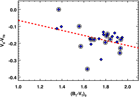
Figure 18.— The conversion from $V_{T}$ to $V$ for late-type stars, plotted as $V_{0}-V_{T0}$ versus $(B_{T}-V_{T})_{0}$. Data for M2 and later classes are circled.

Figure 18 plots the conversion from $V_{T0}$ to $V_{0}$ as a function of $(B_{T}-V_{T})_{0}$:

$$V_{0}-V_{T0}=0.0845-0.149(B_{T}-V_{T})_{0}.$$ (3)

The noise in the data is considerable. It is not related to the double-valued relation between $(B_{T}-V_{T})_{0}$ and $(B-V)_{0}$, as the later spectral classes are not preferentially above or below the line fitted to all of the data.

Table 7Photometry for the bright IRS sample

Target	$B_{T}$	$V_{T}$	$J$	$H$	$K$	Near-IR
	(mag)	(mag)	(mag)	(mag)	(mag)	Reference
$\delta$ Dra	4.322 $\pm$ 0.014	3.165 $\pm$ 0.009	1.191 $\pm$ 0.020	0.837 $\pm$ 0.166	0.464 $\pm$ 0.026	P10, 2MASS
42 Dra	6.345 $\pm$ 0.014	4.955 $\pm$ 0.009	2.696 $\pm$ 0.029	2.197 $\pm$ 0.196	2.019 $\pm$ 0.043	P10, 2MASS
$\xi$ Dra	5.253 $\pm$ 0.014	3.853 $\pm$ 0.009	1.767 $\pm$ 0.022	1.192 $\pm$  $\cdots$	1.038 $\pm$ 0.029	CIO
HR 5755	7.809 $\pm$ 0.015	6.078 $\pm$ 0.009	3.262 $\pm$ 0.138	1.855 $\pm$ 0.212	2.432 $\pm$ 0.126	P10, 2MASS
$\gamma$ Dra	4.246 $\pm$ 0.014	2.381 $\pm$ 0.009	$-$0.443 $\pm$ 0.043	$-$1.160 $\pm$  $\cdots$	$-$1.340 $\pm$ 0.065	CIO
HR 420	7.946 $\pm$ 0.016	6.086 $\pm$ 0.009	3.409 $\pm$ 0.047	2.328 $\pm$ 0.214	2.566 $\pm$ 0.045	P10, 2MASS

Table 8Photometry for M giants observed with the IRS

Target	$B_{T}$	$V_{T}$	$J$	$H$	$K$	Near-IR
	(mag)	(mag)	(mag)	(mag)	(mag)	Reference
HD 13570	9.890 $\pm$ 0.024	7.992 $\pm$ 0.011	4.694 $\pm$ 0.118	4.197 $\pm$ 0.076	3.775 $\pm$ 0.040	2MASS, S04
HD 19554	9.693 $\pm$ 0.021	7.801 $\pm$ 0.011	4.503 $\pm$ 0.107	3.603 $\pm$ 0.236	3.510 $\pm$ 0.118	2MASS, S04
HD 107893	9.970 $\pm$ 0.023	8.014 $\pm$ 0.011	4.686 $\pm$ 0.216	3.761 $\pm$ 0.250	3.613 $\pm$ 0.010	2MASS, S04
HD 17678	10.379 $\pm$ 0.032	8.388 $\pm$ 0.013	4.717 $\pm$ 0.279	3.872 $\pm$ 0.262	3.652 $\pm$ 0.066	2MASS, S04
BD+47 2949	9.895 $\pm$ 0.024	8.017 $\pm$ 0.012	4.810 $\pm$ 0.254	3.850 $\pm$ 0.246	3.614 $\pm$ 0.286	2MASS
HD 206503	10.345 $\pm$ 0.024	8.328 $\pm$ 0.010	4.924 $\pm$ 0.037	4.033 $\pm$ 0.210	3.870 $\pm$ 0.036	2MASS
HD 122755	10.105 $\pm$ 0.027	8.132 $\pm$ 0.012	4.653 $\pm$ 0.236	3.600 $\pm$ 0.216	3.385 $\pm$ 0.224	2MASS
HD 177643	10.561 $\pm$ 0.033	8.642 $\pm$ 0.013	4.972 $\pm$  $\cdots$	3.800 $\pm$ 0.198	3.820 $\pm$ 0.036	2MASS
HD 189246	10.151 $\pm$ 0.032	8.243 $\pm$ 0.014	4.623 $\pm$ 0.320	3.560 $\pm$ 0.228	3.645 $\pm$ 0.322	2MASS, S04
HD 26231	11.060 $\pm$ 0.047	9.093 $\pm$ 0.016	4.582 $\pm$ 0.306	3.611 $\pm$ 0.254	3.451 $\pm$ 0.282	2MASS
HD 127693	11.210 $\pm$ 0.057	9.350 $\pm$ 0.019	5.171 $\pm$ 0.020	4.056 $\pm$ 0.254	4.017 $\pm$ 0.036	2MASS
HD 223306	11.076 $\pm$ 0.043	9.342 $\pm$ 0.017	5.254 $\pm$ 0.021	3.980 $\pm$ 0.236	3.838 $\pm$ 0.232	2MASS
HD 17766	11.261 $\pm$ 0.055	9.242 $\pm$ 0.017	5.125 $\pm$ 0.023	4.365 $\pm$ 0.076	4.107 $\pm$ 0.262	2MASS
HD 32832	10.915 $\pm$ 0.049	8.995 $\pm$ 0.017	4.884 $\pm$ 0.037	4.190 $\pm$ 0.180	3.926 $\pm$ 0.258	2MASS
HD 46396	10.442 $\pm$ 0.033	8.617 $\pm$ 0.014	4.368 $\pm$ 0.254	3.472 $\pm$ 0.230	3.215 $\pm$ 0.061	2MASS, S04
HD 68422	11.135 $\pm$ 0.057	9.268 $\pm$ 0.020	4.421 $\pm$ 0.258	3.407 $\pm$ 0.254	3.117 $\pm$ 0.268	2MASS
HD 74584	10.380 $\pm$ 0.030	8.560 $\pm$ 0.013	4.793 $\pm$ 0.254	3.670 $\pm$ 0.264	3.475 $\pm$ 0.282	2MASS
HD 76386	10.088 $\pm$ 0.028	8.186 $\pm$ 0.013	4.116 $\pm$ 0.201	3.281 $\pm$ 0.238	2.912 $\pm$ 0.045	2MASS, S04
HD 8680	10.944 $\pm$ 0.038	9.147 $\pm$ 0.014	5.187 $\pm$ 0.037	4.201 $\pm$ 0.070	4.027 $\pm$ 0.007	2MASS, CIO
BD+44 2199	11.351 $\pm$ 0.058	9.818 $\pm$ 0.024	4.009 $\pm$ 0.161	3.204 $\pm$ 0.194	2.759 $\pm$ 0.092	2MASS, S04

To determine the $B-V$ and $V-K$ colors of the larger sample, we searched for optical and near-infrared photometry similarly to the SWS sample. Optical photometry in the Johnson system is less homogeneous and less complete than for the SWS sample, so we relied on Tycho magnitudes and the conversions determined above. The bright IRS standards are fainter than the SWS sample, forcing us to rely more on the DIRBE photometry (Price et al., 2010). The IRS M giants are even fainter, and for these we used the calibration of the stellar DIRBE photometry by Smith et al. (2004), which reaches to fainter magnitudes. Generally, though, the near-infrared photometry is less reliable than for the SWS sample. This lack of reliable $JHK$ photometry for reasonably bright sources is one of the outstanding shortcomings in existing catalogs!

Appendix 2. On-line spectroscopy

The spectra presented here are available on-line from the Infrared Science Archive (IRSA) and VizieR. They are organized as simple tables, with columns consisting of wavelength, flux density, uncertainty in flux density, and an integer identifying each spectral segment uniquely (1 for SL1, 2 for SL2, 4 for LL1, and 5 for LL2). IRSA also provides the data in spectral FITS format, which is identical to the simple table format, except the rows and columns are saved as though they were a two-dimensional image. These spectra are also available from the first author’s website.

References

- Ardila et al. (2010) Ardila, D. R., Van Dyk, S. D., Makowiecki, W., et al. 2010, ApJS, 191, 301
- Appenzeller (1967) Appenzeller, I. 1967, PASP, 79, 102
- Beichman et al. (1988) Beichman, C. A., Neugebauer, G., Habing, H. J., Clegg, P. E., & Chester, T. J. 1988, Infrared Astronomical Satellite (IRAS) Catalogs and Atlases Explanatory Supplement (Pasadena: JPL)
- Bessell (2000) Bessell, M. 2000, PASP, 112, 773
- Bidelman (1954) Bidelman, W. P. 1954, ApJS, 1, 175
- Blanco (1954) Blanco, V. M. 1954, AJ, 59, 396
- Buscombe (1962) Buscombe, W. 1962, Mt. Stromlo Obs. Mimeo, 4, 1
- Chiar & Tielens (2006) Chiar, J. E., & Tielens, A. G. G. M. 2006, ApJ, 637, 774
- Cohen et al. (1992a) Cohen, M., Walker, R. G., & Witteborn, F. C. 1992a, AJ, 104, 2030
- Cohen et al. (1992b) Cohen, M., Witterborn, F. C., Carbon, D. F., et al. 1992b, AJ, 104, 2045
- de Vaucouleurs (1956) de Vaucouleurs, A. 1956, MNRAS, 116, 277
- Drimmel et al. (2003) Drimmel, R., Cabrera-Lavers, A., & López-Corredoira, M. 2003, A&A, 409, 205
- Eggen (1955) Eggen, O. J. 1955, AJ, 60, 65
- Eggen (1957) Eggen, O. J. 1957, Obs., 77, 229
- Eggen (1960) Eggen, O. J. 1960, MNRAS, 120, 448
- Engelke (1992) Engelke, C. W. 1992, AJ, 104, 1248
- Engelke et al. (2006) Engelke, C. W., Price, S. D., & Kraemer, K. E. 2006, AJ, 132, 1445
- Gezari et al. (2000) Gezari, D. Y., Pitts, P. S., & Schmitz, M. 2000, Catalog of Infrared Observations, Version 5.1 (Greenbelt, MD: NASA/Goddard Space Flight Center)
- Gillett & Merrill (1975) Gillett, F. C., & Merrill, K. M. 1975, Icarus, 26, 358
- Grasdalen & Gaustad (1971) Grasdalen, G. L., & Gaustad, J. E. 1971, AJ, 76, 231
- Haggkvist & Oja (1970) Haggkvist, L., & Oja, T. 1970, private comm. to Simbad
- Heras et al. (2002) Heras, A. M., Shipman, R. F., Price, S. D., et al. 2002, A&A, 394, 539
- Høg et al. (2000) Høg, E., Fabricius, C., Makarov, V. V., et al. 2000, A&A, 355, L27
- Houck et al. (2004) Houck, J. R., Roellig, T. L., van Cleve, J., et al. 2004, ApJS, 154, 18
- Houk (1978) Houk, N. 1978, Michigan Catalogue of Two-Dimensional Spectral Types for the HD Stars. Vol. 2 (Ann Arbor, MI: Univ. of Michigan)
- Houk (1982) Houk, N. 1982, Michigan Catalogue of Two-Dimensional Spectral Types for the HD Stars. Vol. 3 (Ann Arbor, MI: Univ. of Michigan)
- Houk & Cowley (1975) Houk, N., & Cowley, A. P. 1975, Univ. of Michigan Catalogue of Two-Dimensional Spectral Types for the HD Stars. Vol. I (Ann Arbor, MI: Univ. of Michigan)
- Houk & Smith-Moore (1988) Houk, N., & Smith-Moore, M. 1988, Michigan Catalogue of Two-dimensional Spectral Types for the HD Stars. Vol. 4 (Ann Arbor, MI: Univ. of Michigan)
- Hoyle & Wilson (1958) Hoyle, F., & Wilson, O. C. 1958, ApJ, 128, 604
- Johnson et al. (1966) Johnson, H. L., Iriarte, B., Mitchell, R. I., & Wisniewski, W. Z. 1966, Comm. Lunar Plan. Lab., 4, 99
- Jones (1972) Jones, D. H. P. 1972, ApJ, 178, 467
- Keenan (1942) Keenan, P. C. 1942, ApJ, 95, 461
- Keenan (1954) Keenan, P. C. 1954, ApJ, 120, 484
- Keenan & Hynek (1945) Keenan, P. C., & Hynek, J. A. H. 1945, ApJ, 101, 265
- Keenan & McNeil (1989) Keenan, P. C., & McNeil, R. C. 1989, ApJS, 71, 245
- Kraemer et al. (2002) Kraemer, K. E., Sloan, G. C., Price, S. D., & Walker, H. J. 2002, ApJS, 140, 389.
- Lee (1970) Lee, T. A. 1970, ApJ, 162, 217
- Lutz (1971) Lutz, T. E. 1971, PASP, 83, 488
- Morgan (1938) Morgan, W. W. 1938, ApJ, 87, 460
- Morgan et al. (1953) Morgan, W. W., Harris, D. L., & Johnson, H. L. 1953, ApJ, 118, 92
- Morgan & Keenan (1973) Morgan, W. W., & Keenan, P. C. 1973, ARA&A, 11, 29
- Morgan et al. (1943) Morgan, W. W., Keenan, P. C., & Kellman, E. 1943, Astrophys. Monographs (Chicago: Univ. Chicago Press)
- Moshir et al. (1992) Moshir, M., et al. 1992, Explanatory Supplement to the IRAS Faint Source Survey, ver. 2, JPL D-10015 8/92 (Pasadena: JPL)
- Nassau & van Albada (1947) Nassau, J. J., & van Albada, G. B. 1947, ApJ, 106, 20
- Nicolet (1978) Nicolet, B. 1978, A&AS, 34, 1
- Oschenbein (1980) Oschenbein, F. 1980, Bull. Inf. Centre Donnees Stellaires, 19, 74 (SAO Catalog)
- Price et al. (2010) Price, S. D., Smith, B. J., Kuchar, T. A., Mizuno, D. R., & Kraemer, K. E. 2010, ApJS, 190, 203
- Ramirez et al. (2014) Ramirez, R. M., Kopparapu, R., Zugger, M. E., et al. 2014, Nature Geoscience, 7, 59
- Rieke & Lebofsky (1985) Rieke, G. H., & Lebofsky, M. J. 1985, ApJ, 288, 618
- Roman (1952) Roman, N. G. 1952, ApJ, 116, 122
- Rothman et al. (2010) Rothman, L. S., Gordon, I. E., Barber, R. J., et al. 2010, J. Quant. Spectrosc. and Rad. Transfer, 111, 2139
- Rothman et al. (2012) Rothman, L. S., Gordeon, I. E., Babikov, I. E., et al. 2012, J. Quant. Spectrosc. and Rad. Transfer, 130, 4
- Ryde et al. (2002) Ryde, N., Lambert, D. L., Richter, M. J., & Lacy, J. H. 2002, ApJ, 580, 447
- Ryde et al. (2006) Ryde, N., Richter, M. J., Harper, G. M., Eriksson, K., & Lambert, D. L. 2006, ApJ, 645 652
- Ryde et al. (2015) Ryde, N., Lambert, J., Farzone, M., et al. 2015, A&A, 573, 28
- Schlafly & Finkbeiner (2011) Schlafly, E. F., & Finkbeiner, D. P. 2011, ApJ, 737, 103
- Sharpless (1952) Sharpless, S. 1952, ApJ, 116, 251
- Skrutskie et al. (2006) Skrutskie, M. F., Cutri, R. M., Stiening, R., et al. 2006, AJ, 131, 1163
- Sloan et al. (2015) Sloan, G. C., Herter, T. L., Charmandaris, V., Sheth, K., Burgdorf, M., & Houck, J. R. 2015, AJ, 149, 11 (Paper I)
- Sloan et al. (2003b) Sloan, G. C., Kraemer, K. E., Price, S. D., & Shipman, R. F. 2003b, ApJS, 147, 379
- Sloan & Ludovici (2012) Sloan, G. C., & Ludovici, D. 2012, IRS-TR 12001: Spectral Pointing-Induced Througput Error and Spectral Shape in Short-Low Order 1 (Ithaca, NY: Cornell)
- Sloan et al. (2003a) Sloan, G. C., Nerenberg, P. S., & Russell, M. R. 2003a, IRS-TR 03001: The Effect of Spectral Pointing-Induced Throughput Error on Data from the IRS (Ithaca, NY: Cornell)
- Smith et al. (2004) Smith, B. J., Price, S. D., & Baker, R. I. 2004, ApJS, 154, 673
- Stoy (1959) Stoy, R. H. 1959, Monthly Notices Astron. Soc. S. Africa, 18, 48
- Tabur et al. (2009) Tabur, V., Kiss, L. L., & Bedding, T. R. 2009, ApJ, 703, L72
- Tsuji (2000) Tsuji, T. 2000, ApJ, 540, L99
- Tsuji (2001) Tsuji, T. 2001, A&A, 376, L1
- Tsuji et al. (1997) Tsuji, T., Ohnaka, K., Aoki, W., Yamamura, Y., 1997, A&A, 320, L1
- Tsuji (2009) Tsuji, T. 2009, A&A, 504, 543
- Upgren (1960) Upgren, A. R. 1960, AJ, 65, 644
- van Leeuwen (2007) van Leeuwen, F. 2007, Hipparcos, the New Reduction of the Raw Data (Berlin: Springer)
- Van Malderen et al. (2004) Van Malderen, R., Decin, L., Kester, D., et al. 2004, A&A, 414, 677
- Werner et al. (2004) Werner, M. W., Roellig, T. L., Low, F. J., et al. 2004, ApJS, 154, 1
- Wilson & Bappu (1957) Wilson, O. C., & Bappu, V. M. K. 1957, ApJ, 125, 661
- Wordsworth et al. (2010) Wordsworth, R., Forget, F., & Eymet, V., Icarus, 210, 992