Abstract. The possible control of competitive invasion by infection of the invader and multiplicative noise is studied. The basic model is the Lotka-Volterra competition system with emergent carrying capacities. Several stationary solutions of the non-infected and infected system are identified as well as parameter ranges of bistability. The latter are used for the numerical study of invasion phenomena. The diffusivities, the infection but in particular the white and colored multiplicative noise are the control parameters. It is shown that not only competition, possible infection and mobilities are important drivers of the invasive dynamics but also the noise and especially its color and the functional response of populations to the emergence of noise.

Key words: Eco-epidemiological model, explicit and emergent carrying capacities, bioinvasion, resident–invader competition, biocontrol, infection, standard incidence, diffusion, multiplicative noise, colored noise, functional response to noise

AMS subject classification: 35K57, 35Q92, 60H15

1. Introduction

The main aim of modeling biological population dynamics is to improve the understanding of the functioning of food chains and webs as well as their dependence on internal and external conditions. Hence, mathematical models of biological population dynamics have not only to account for growth and interactions but also for spatiotemporal processes like random or directed and joint or relative motion of species, as well as the heterogeneity of the environment. Early attempts began with statistics, exponential growth, physico-chemical (neutral) diffusion, and Lotka-Volterra type interactions. These approaches have been continuously refined to more realistic descriptions of the development of natural populations.
Ecological and epidemiological models are known since more than 200 years. First attempts to merge these models appeared only about 30 years ago, cf. [1, 13, 7, 9] as well as [55, 56]. Infectious diseases are prominent examples of biological invasions and continue to (re-)emerge in modern times. The negative econo-ecological effects of bioinvasions [6, 41] have led to a remarkable hype of bioinvasion research incl. modeling, cf. [37, 15, 59, 45, 43]. The history of research on stochastic processes and integration is long as well, historical surveys have been published, cf. [18, 34]. The seminal work by Îto [17] and Stratonovich [51] should be particularly recognized.
The present, to a large extent numerical study combines aspects of spatial eco-epidemiology and environmental stochasticity, namely the diffusive invasion of an alien species, its competition with the indigenous resident, and its biocontrol through targeted infection in a noisy environment. Contrary to previous publications [25, 26], the environmental variability is modeled as external multiplicative noise, in some cases with a certain functional response of the populations.

Modeling environmental variability with multiplicative white noise goes back to the 1970s. Not only did May [30, 31] introduce the model that is used until today as a perturbation of the growth rate of a population by “white noise” but only a few years later, a more mechanistic basis of this model was developed. Branching processes provide a stochastic model that describes the number of offspring for a given number of individuals $Z_{i}$ within one generation $i$. The population number $Z_{i+1}$ in generation $i+1$ is updated for a given population $Z_{i}$ according to previously chosen probability distributions. This model was extended by Smith and Wilkinson [49, 50] by a stochastic process $\zeta_{i}$ which modulates for each new generation the offspring that is generated. Branching processes in random environments (BPRE) provide an individual-based model for population growth. For large population numbers, a BPRE can be approximated by a stochastic differential equation (SDE) that accounts both for demographic as well as environmental stochasticity. Keiding [20] conjectured the form of the resulting diffusion approximation, his conjecture was rigorously proven by Kurtz [23]. The model introduced by May is obtained from Kurtz’ diffusion approximation by neglecting the term due to demographic stochasticity. Thus, the SDE model for environmental stochasticity is derived from the influence of a random environment on the population dynamics of a branching process but neglects its demographic stochasticity.

In this study we consider the properties of environmental variability in more detail. The multiplicative noise term implies that the effect of environmental fluctuations on the individuals of a population is additive. Whereas this seems reasonable for small population densities we propose that for large population numbers the effect of individual responses to environmental fluctuations on the population should decrease. Thus, we propose that the population-dependent response to environmental noise saturates for large population numbers similar to the functional response of predators at large prey densities and therefore we model the population-dependent response to environmental noise in a completely analogous way.

The subject of our study is the influence of environmental stochasticity on a biological invasion. In order to account for spatial spread we extend our system of SDEs by diffusion terms so that we obtain a system of stochastic reaction-diffusion equations. Spatiotemporal environmental fluctuations are represented by time-dependent random fields. In contrast to previous studies, we consider random fields that are correlated both in space and in time, i.e., spatiotemporally colored noise.

The assumption of uncorrelated white noise is usually justified by the coarseness of temporal or spatial scale, respectively. If spatial or temporal correlation length are much shorter than the time or length scale of interest, it seems valid to consider the time-dependent random field as uncorrelated. However, particular care must be taken when considering spatiotemporal dynamics driven by noise. Stochastic differential equations driven by uncorrelated noise can usually solved over a function space such as $L^{2}$ and this remains true if the system is extended to a reaction-diffusion equation over one-dimensional space ($d=1$). But for spatial dimensions $d\geq 2$ solutions for stochastic reaction-diffusion equations driven by uncorrelated noise can only be guaranteed in a space of generalised functions, see e.g. [58, 38]. The reason for this phenomenon is that the Laplacian cannot smooth uncorrelated noise sufficiently for spatial dimensions exceeding 1 so that a solution may contain peaks resembling the $\delta$ distribution. Not only is the physical significance of these solutions debatable but also numerical approximations are not capable of capturing this aspect of the continuous system. Here we take a pragmatic point of view on this difficult problem and present numerical solutions for temporally and spatially white noise where the space may be interpreted as a discrete lattice whose nodes interact by a discrete Laplacian.

2. Resident-invader competition with infection in the invader population

For the invasion of a resident population by a competing invader, the Lotka-Volterra competition model is used, i.e.,

$$\frac{dN_{1}}{dt} =r_{1}N_{1}-c_{11}N_{1}^{2}-c_{12}N_{1}N_{2},$$ (2.1)

$$\frac{dN_{2}}{dt} =r_{2}N_{2}-c_{22}N_{2}^{2}-c_{21}N_{1}N_{2},$$ (2.2)

where $N_{1}$ and $N_{2}$ are resident and invader respectively. Carrying capacities will not explicitely be introduced because they can suppress a higher variety of solutions and rather appear as special cases [8, 22, 28, 46]. The $r$’s stand for the growth rates and the $c$’s for the inter- and intraspecific competition.

A specific infection of the invading population can be used as biocontrol measure to stop and reverse the invasion, cf. [14, 19, 33, 5]. To model this, the invader population is split into susceptibles $S$ and infecteds $I$,

$$N_{2}=S+I.$$

Then, the local dynamics reads with notation $\mathbf{X}=\{X_{1}\equiv N_{1},X_{2}=S,X_{3}=I\}$

$$\frac{dX_{1}}{dt} =f_{1}\,(\mathbf{X})=r_{1}X_{1}-c_{11}X_{1}^{2}-c_{12}X_{1}(X_{2}+X_{3}),$$ (2.3)

$$\frac{dX_{2}}{dt} =f_{2}\,(\mathbf{X})=r_{2}X_{2}-c_{22}X_{2}(X_{2}+X_{3})-c_{21}X_{1}X_{2}-\lambda\frac{X_{2}X_{3}}{(X_{2}+X_{3})^{q}},$$ (2.4)

$$\frac{dX_{3}}{dt} =f_{3}\,(\mathbf{X})=r_{2}X_{3}-c_{22}X_{3}(X_{2}+X_{3})-c_{21}X_{1}X_{3}+\lambda\frac{X_{2}X_{3}}{(X_{2}+X_{3})^{q}}-\mu X_{3}\,,$$ (2.5)

where $\lambda$ is the transmission coefficient of the disease and $\mu$ the disease-induced higher mortality rate of the infecteds. The exponent $q$ allows to describe mass-action type ($q=0$) and frequency-dependent transmission ($q=1$) of the disease respectively [1, 32].

However, one cannot expect that growth rates and competition intensities of susceptibles and infecteds are the same. They should rather be split and could be ordered like

$$\begin{array}[]{llclc}r_{2}&\Rightarrow&\{r_{2},r_{3}\}&\leavevmode\nobreak\ \textrm{\&}\nobreak\leavevmode&r_{3}\leq r_{2}\,,\\ c_{12}&\Rightarrow&\{c_{12},c_{13}\}&\leavevmode\nobreak\ \textrm{\&}\nobreak\leavevmode&c_{13}\leq c_{12}\,,\\ c_{21}&\Rightarrow&\{c_{21},c_{31}\}&\leavevmode\nobreak\ \textrm{\&}\nobreak\leavevmode&c_{21}\leq c_{31}\,,\\ c_{22}&\Rightarrow&\{c_{22},c_{23},c_{32},c_{33}\}&\leavevmode\nobreak\ \textrm{\&}\nobreak\leavevmode&c_{23}\leq c_{33}\leq c_{22}\leq c_{32}\,.\end{array}$$ (2.10)

The ordering of the intra- and interspecific competition coefficients of susceptibles and infecteds depends on the biological species, cf. [2]. However, it can be certainly accepted [46] that

$$c_{23}\leq c_{22}\wedge c_{33}\leq c_{32}\,.$$

System (2.3–2.5) then changes to

$$\frac{dX_{1}}{dt} =f_{1}(\mathbf{X})=(r_{1}-c_{11}X_{1})X_{1}-(c_{12}X_{2}+c_{13}X_{3})X_{1}\,,$$ (2.11)

$$\frac{dX_{2}}{dt} =f_{2}(\mathbf{X})=(r_{2}-c_{22}X_{2})X_{2}-(c_{21}X_{1}+c_{23}X_{3})X_{2}-\lambda\frac{X_{2}X_{3}}{(X_{2}+X_{3})^{q}},$$ (2.12)

$$\frac{dX_{3}}{dt} =f_{3}(\mathbf{X})=(r_{3}-\mu-c_{33}X_{3})X_{3}-(c_{31}X_{1}+c_{32}X_{2})X_{3}+\lambda\frac{X_{2}X_{3}}{(X_{2}+X_{3})^{q}}\,.$$ (2.13)

For convenience, the model of the local dynamics is not analysed in terms of $X_{1}$, $X_{2}$ and $X_{3}$ but rather in $X_{1}$, $i$ and $N_{2}=X_{2}+X_{3}$ where $i$ is the prevalence, i.e., the infected fraction of the total invader population $N_{2}$ [16],

$$i=\frac{X_{2}}{X_{2}+X_{3}}=\frac{X_{2}}{N_{2}}.$$

Having in mind that

$$\frac{di}{dt}=\frac{1}{N_{2}}\left(\frac{dX_{2}}{dt}-i\frac{dN_{2}}{dt}\right)\,,$$ (2.14)

it follows

$$\frac{dX_{1}}{dt} =r_{1}X_{1}-c_{11}X_{1}^{2}-\left[c_{12}(1-i)+c_{13}i\right]X_{1}N_{2}\,,$$ (2.15)

$$\frac{di}{dt} =\left\{r_{3}-r_{2}+\lambda N_{2}^{1-q}-\mu+N_{2}\left[(c_{22}-c_{32})(1-i)+(c_{23}-c_{33})i\right]+X_{1}\left[c_{21}-c_{31}\right]\right\}\,*\leavevmode\nobreak\ \leavevmode\nobreak\ \leavevmode\nobreak\ \leavevmode\nobreak\ \leavevmode\nobreak\ \leavevmode\nobreak\$$

$$\leavevmode\nobreak\ \leavevmode\nobreak\ \leavevmode\nobreak\ \leavevmode\nobreak\ \leavevmode\nobreak\ *i(1-i)\,,$$ (2.16)

$$\frac{dN_{2}}{dt} =\left\{G(N_{2},i)-\left[c_{21}(1-i)+c_{31}i\right]X_{1}\right\}N_{2}\,,$$ (2.17)

with

$$G(N_{2},i)=r_{2}(1-i)+(r_{3}-\mu)i-N_{2}\left[c_{22}(1-i)^{2}+(c_{23}+c_{32})i(1-i)+c_{33}i^{2}\right]\,.$$ (2.18)

The latter expression is also found for predator-prey systems with infected prey [46]. Note that if the resident $X_{1}$ resp. the predator in [46] cannot distinguish between susceptible and infected invader resp. prey, the temporal change of the prevalence becomes independent of the type of interspecific ecological interactions such as competition and predation. It only contains terms describing the intraspecific competition of susceptibles and infecteds in the infected population.

2.1. Stationary solutions and stability for frequency-dependent (standard) incidence q=1

In phytopathology, the transmission of especially fungal diseases is described with standard incidence [54]. A corresponding model of the invasion of a fungal disease over a vineyard has been investigated in [4]. Further on, only the standard incidence is considered, i.e., $q=1$.

The infection-free system, i.e., $i\equiv 0,N_{2}=X_{2}$, is the Lotka-Volterra competition model with its known stationary solutions and their stability ranges. Especially interesting for the consideration of spatial invasions is the bistable parameter range

$$r_{1}c_{22}-r_{2}c_{12}>0\leavevmode\nobreak\ \wedge\leavevmode\nobreak\ r_{2}c_{11}-r_{1}c_{21}>0\,,$$

when both the invader-free $(\dfrac{r_{1}}{c_{11}},0,0)$ and the resident-free $(0,0,\dfrac{r_{2}}{c_{22}})$ states are stable and can compete for space. The opposite case may also happen: The invader arrives already infected, i.e., $i\equiv 1,N_{2}=X_{3}$, and the invader-free $(\dfrac{r_{1}}{c_{11}},0,0)$ and the resident-free $(0,0,\dfrac{r_{3}-\mu}{c_{33}})$ states can be both at once stable for

$$r_{1}c_{33}-(r_{3}-\mu)\,c_{13}>0\leavevmode\nobreak\ \wedge\leavevmode\nobreak\ (r_{3}-\mu)\,c_{11}-r_{1}c_{31}>0\,.$$

However, the latter as well as the possible bistability of resident-only $(\dfrac{r_{1}}{c_{11}},0,0)$ and (susceptible-infected)-invader-only $(0,i^{S1},N_{2}^{S1})$ states will not be considered here.

2.2. Spatiotemporal dynamics in a variable environment

The main focus of this study is to consider the spatiotemporal effects of a more detailed model of environmental variability. We assume that all species spread randomly so that mobility can be described as diffusion with coefficients $\mathbf{D}=\{D_{ii}=D_{i}\,;\leavevmode\nobreak\ D_{ij}\equiv 0\leavevmode\nobreak\ \forall i\neq j\,;\leavevmode\nobreak\ i,j=1,2,3\}$. Also we add Gaussian random fields $\boldsymbol{\xi}(\vec{r},t)=\{\xi_{i}(\vec{r},t)\,;\leavevmode\nobreak\ i=1,2,3\}$ to system (2.11–2.13) so that we obtain the system of stochastic partial differential equations

$$\frac{\partial\mathbf{X}(\vec{r},t)}{\partial t}-\mathbf{D}\Delta\mathbf{X}(\vec{r},t)=\mathbf{f}\left[\mathbf{X}(\vec{r},t)\right]+\mathbf{g}\left[\mathbf{X}(\vec{r},t)\right]\,\boldsymbol{\xi}(\vec{r},t)\,,$$ (2.19)

where the matrix function $\mathbf{g}(\mathbf{X})=\{g_{ij}(\mathbf{X});\leavevmode\nobreak\ i,j=1,2,3\}$ determines the density-dependent noise intensity. We consider horizontal processes with position vector $\vec{r}=\{x,y\}$ and corresponding Laplace operator $\Delta=\partial^{2}/\partial x^{2}+\partial^{2}/\partial y^{2}$. In literature, often temporally and spatially uncorrelated “white” Gaussian fields with zero mean and delta correlation have been considered

$$\left<\xi_{i}(\vec{r},t)\right>=0\,,\leavevmode\nobreak\ \left<\xi_{i}(\vec{r}_{1},t_{1})\,\xi_{i}(\vec{r}_{2},t_{2})\right>=\delta(\vec{r}_{1}-\vec{r}_{2})\,\delta(t_{1}-t_{2})\,,\leavevmode\nobreak\ i=1,2,3\,.$$ (2.20)

Here, we investigate the effect of extending this model by correlated “colored” noise with correlation lenghts $\tau$ and $\lambda$ in the temporal and spatial domain, respectively. Apart from using colored noise we also investigate a generalisation of the density-dependent noise $\mathbf{g}\left(\mathbf{X}\right)$. Purely diagonal, linear multiplicative noise

$$g_{ii}(\mathbf{X})=\omega_{ii}X_{i}\,;\leavevmode\nobreak\ g_{ij}(\mathbf{X})=0\leavevmode\nobreak\ \forall\leavevmode\nobreak\ i\neq j\,;\leavevmode\nobreak\ i,j=1,2,3\,;$$ (2.21)

can be interpreted as a model where individuals respond independently to stochastic environmental variability. Thus, the effect of environmental fluctuations on each individual directly translates into variability at the population level – the response at the population level is additive. The alternative model suggested here is based on the assumption that in large populations individuals do not repond to fluctuations independently from each other. Instead we propose that larger populations respond to environmental variability in a more robust way, i.e., neither favourable nor adverse effects influence the population proportional to the number of individuals:

$$g_{ij}(\mathbf{X})=\dfrac{\omega_{ij}X_{j}^{m}}{\gamma_{ij}+\sum\limits_{k=1}^{3}\,a_{ik}X_{k}^{n}}\,;\leavevmode\nobreak\ i,j=1,2,3\,;\leavevmode\nobreak\ 1\leq m\leq n\leq 2\,.$$ (2.22)

For $m=n$, the parameter $\omega_{ij}/a_{ij}$ is the maximum noise intensity that is reached asymptotically for large populations $X_{j}$. The parameter $\gamma_{ij}$ is the population level at which the noise intensity reaches half of the maximum level $\omega_{ij}/a_{ij}$. Thus, this parameter describes the ability of a population to collectively reduce the effect of noise – the higher $\gamma_{ij}$, the higher the population level must be until population $X_{j}$ is appreciably affected by environmental variability.

For $m<n$, the noise intensity even decreases and eventually vanishes for high population densities. However, these values are never reached.

In previous papers [25, 26], it was shown that a certain variability of the environment and the mobilities of the competitors are the system-driving forces. Extreme events such as landslides lead to bare ground re-invadable by both resident and alien species. These events at random times, size and locations are not considered here. They are replaced by white and colored noises [42, 47, 48]. Again, the biocontrol of the invasion through a specific infection of the non-indigenous species is studied.

3. Numerical methods

The numerical solution of stochastic partial differential equations is a difficult problem and the subject of current research. For this reason we explain how the spatiotemporal model (2.19) can be solved numerically and how spatiotemporally correlated noise can be generated. We follow a finite difference approach where in a first step the spatial domain is discretised. In this way the system of stochastic partial differential equation is approximated by uncoupled stochastic differential equations that are solved numerically in a second step. For the first step, we use the semi-implicit Peaceman-Rachford method [40, 52] which, in particular for stochastic equations, often seems to be more robust than the simplest explicit scheme. In the following we will explain how the discretised system can be solved using the derivative-free Milstein method and how spatiotemporally correlated noise can be generated.

3.1. Derivative-free Milstein method

For numerical integration, the derivative-free Milstein method is used, cf. [35, 36, 21] but also the short descriptions [44, 10]. Sometimes and in particular for the purpose of this study, it is even sufficient to consider purely diagonal intensity matrices

$$g_{ii}(\mathbf{X})=\dfrac{\omega_{ii}X_{i}^{m}}{\gamma_{ii}+a_{ii}X_{i}^{n}}\,;\leavevmode\nobreak\ a_{ii}\equiv 1\,;\leavevmode\nobreak\ i=1,2,3\,;\leavevmode\nobreak\ 1\leq m\leq n\leq 2\,.$$ (3.1)

Then, the Milstein scheme reads with time step $\Delta t$ and Stratonovich interpretation

$$X_{t+\Delta t}^{i} =X_{t}^{i}+f_{i}(X_{t}^{i})\Delta t+g_{ii}(X_{t}^{i})\Delta W_{i}+\dfrac{1}{2\sqrt{\Delta t}}\left[g_{ii}(\bar{X}_{t}^{i})-g_{ii}(X_{t}^{i}\right](\Delta W_{i})^{2}\,,$$ (3.2)

with

$$\bar{X}_{t}^{i} =X_{t}^{i}+f_{i}(X_{t}^{i})\Delta t+g_{ii}(X_{t}^{i})\sqrt{\Delta t}\,,$$

and

$$\Delta W_{i} =W_{t+\Delta t}^{i}-W_{t}^{i}\sim\sqrt{\Delta t}\,\mathcal{N}(0,1)\,.$$

As usual, $\mathcal{N}(0,1)$ stands for the normal distribution with zero mean and unity variance. The required uniformly distributed random numbers are generated with the Mersenne Twister [29], the normally distributed with the common Box-Muller algorithm [3].

3.2. Generation of correlated Gaussian random fields

García-Ojalvo and Sancho [12, 11] developed a method for generating spatially and temporally colored noise from the stochastic reaction-diffusion equation

$$\frac{\partial\zeta(\vec{r},t)}{\partial t}=\frac{\lambda^{2}}{\tau}\Delta\zeta(\vec{r},t)-\frac{1}{\tau}\zeta(\vec{r},t)+\frac{1}{\tau}\eta(\vec{r},t)$$ (3.3)

Here, the term $\eta(\vec{r},t)$ stands for uncorrelated (white) noise. The parameters $\tau$ and $\lambda$ determine the correlation lengths in the temporal and the spatial domain, respectively. In addition, a scaling factor $\epsilon$ for the variance of normally-distributed random variables in Fourier space has to be chosen. The authors introduce Eq. (3.3) as an analogon of the Ohrnstein-Uhlenbeck process which is the solution of (3.3) without the spatial term $\dfrac{\lambda^{2}}{\tau}\Delta\zeta(r,t)$. But it has to be noted that for two-dimensional space (and spatial dimensions exceeding two) the solutions of equation (3.3) will be generalised functions rather than functions in a space such as $L^{2}$. Thus, strictly speaking, we are generating discrete spatiotemporally colored random fields that are derived from the model (3.3) without being approximate solutions of the continuous problem.

The spatiotemporal random field $\zeta(\vec{r},t)$ is simulated by transforming a discretised version $\zeta_{ij}(t)$ of (3.3) to Fourier space:

$$\zeta_{\mu\nu}(t)=(\Delta x)^{2}\sum_{i,j=1}^{L}\exp(-\mathbf{i}k\cdot\vec{r})\zeta_{ij}(t)$$ (3.4)

We denote the discrete Fourier transform $\zeta_{\mu\nu}(t)$ with greek indices $\mu$, $\nu$ rather than $i$, $j$ and the coordinate $k$ in frequency space is

$$k=\frac{2\pi}{L\Delta x}(\mu,\nu),\qquad\mu,\nu=0,\dots,L-1.$$

Then the Fourier transformed field $\zeta_{\mu\nu}(t)$ at the next time step $t+\Delta t$ is calculated by

$$\zeta_{\mu\nu}(t+\Delta t) =\zeta_{\mu\nu}(t)\exp\left(-\frac{c_{\mu\nu}}{\tau}\Delta t\right)+\sqrt{\frac{\epsilon(L\Delta x)^{2}}{\tau c_{\mu\nu}}\left[1-\exp\left(-\frac{c_{\mu\nu}}{\tau}\Delta t\right)\right]}\alpha_{\mu\nu}$$ (3.5)

Here, $\alpha_{\mu\nu}$ is the Fourier transform of an uncorrelated Gaussian noise field $\alpha_{ij}$. The efficiency of this method is increased by directly generating the Fourier transformed field $\alpha_{\mu\nu}$. The (complex-valued) discrete Fourier transform $\alpha_{\mu\nu}$ of real-valued fields $\alpha_{ij}$ obeys some symmetries that lead to the following restrictions:

$$\alpha_{\mu\nu} =\alpha_{L-\mu,L-\nu}^{*}$$ (3.6)

$$\alpha_{\mu\nu} \in\mathbb{R},\quad\text{for }\mu,\nu=0,\frac{L}{2}$$ (3.7)

where $z^{*}$ denotes the complex conjugate of $z\in\mathbb{C}$. The condition (3.6) means that $\alpha_{\mu\nu}$ have the same real part as $\alpha_{L-\mu,L-\nu}$ found by reflecting through the centre ($\mu=\nu=1/2$) whereas the imaginary parts only differ by opposite signs.

Also in (3.5), $c_{\mu\nu}$ is the Fourier transform of the discretisation of the differential operator  $\mathcal{L}=\operatorname{id}-\lambda^{2}\Delta$:

$$c_{\mu\nu}=1-\frac{2\lambda^{2}}{(\Delta x)^{2}}\left[\cos\left(\frac{2\pi\mu}{L}\right)+\cos\left(\frac{2\pi\nu}{L}\right)-2\right].$$ (3.8)

For further details on the derivation of this method, we refer the reader to [11] or [12].

4. Resident-invader competition-diffusion model with infected invader in a variable environment

4.1. Local dynamics with multiplicative white noise and induced transitions

Not surprising and like for $q=0$ [57, 53], Lehmann [24] and Woyzichovski [60] found disease-induced oscillations for $q=1$ as well. Their interesting result was that there may be bistability of the resident-only state and the limit cycle when coexisting resident, susceptible and infected invaders oscillate, cf. Figure 1. The following parameters have been used for the latter setting:

$$r_{1} =1.2500\,,\leavevmode\nobreak\ r_{2}=1.0000\,,\leavevmode\nobreak\ r_{3}=0.6775$$

$$c_{11}=0.5000\,,\leavevmode\nobreak\ c_{12} =0.8500\,,\leavevmode\nobreak\ c_{21}=0.4250\,,\leavevmode\nobreak\ c_{13}=0.5000\,,\leavevmode\nobreak\ c_{31}=0.5000$$ (4.1)

$$c_{22} =0.6000\,,\leavevmode\nobreak\ c_{23}=0.4000\,,\leavevmode\nobreak\ c_{32}=0.6010\,,\leavevmode\nobreak\ c_{33}=0.5000$$

$$\lambda =0.4000\,,\leavevmode\nobreak\ \mu=0.0250$$

All other semi-trivial states turn out to be unstable for this parameter range.

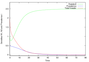
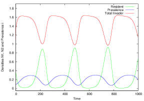
Figure 1: Bistability of resident-only state and oscillating coexistence

Now, one effect of white noise in locally multiple stable systems is shown, i.e., the switch from one stable attractor to the other for sufficiently but not too high noise intensity. For simplicity, the linear density dependence (2.21) of the intensity is chosen, which has been successfully applied to numerous cases. Here, the leaving of the initial limit cycle is demonstrated.

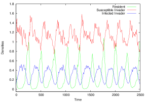
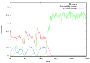
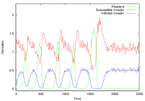
Figure 2: Noise-induced transitions from oscillating coexistence to resident-only state resp. resident extinction. Linear density dependence (2.21) with $\omega_{ii}=0.1\,\leavevmode\nobreak\ i=1,2,3$ .

The three subfigures of Figure 2 show typical outcomes of hundreds of simulations with different seeds of the random number generator. The left subfigure shows the persistence of the limit cycle whereas the middle demonstrates the expected leaving of the cycle for the other stable stationary solution, i.e., the resident-only state. The result in the right subfigure appeared a bit unexpected, however, due to some catastrophic shift, the resident died out and the remaining susceptible and infected invader survived. One should have in mind that the latter $(0,X_{2}^{s},X_{3}^{s})$ state is unstable to the reintroduction of the resident.

4.2. Invasions and noise I

4.2.1. Linear noise and biocontrol of invasion

For the beginning, the results in the mentioned previous papers [25, 26], where simulated landslides led to bare land competitively re-invadable by resident and invader, are reproduced with external noise. The initial condition is a “red” invader patch at its emergent carrying capacity $r_{22}/c_{22}$ at the “upper left corner” of the “green” habitat of the native species at $r_{11}/c_{11}$. This patch should exceed the related critical patch size. Otherwise it will simply decay regardless of its competitive strength and mobility [39, 27]. Zero-flux boundary conditions are applied.

The linear noise (2.21) and parameters from the previous publications have been taken:

$$r_{1} =1.000\,,\leavevmode\nobreak\ r_{2}=1.000\,,\leavevmode\nobreak\ r_{3}=0.800$$

$$c_{11}=1.000\,,\leavevmode\nobreak\ c_{12} =1.300\,,\leavevmode\nobreak\ c_{21}=1.200\,,\leavevmode\nobreak\ c_{13}=1.299\,,\leavevmode\nobreak\ c_{31}=1.201$$

$$c_{22} =0.999\,,\leavevmode\nobreak\ c_{23}=0.998\,,\leavevmode\nobreak\ c_{32}=1.001\,,\leavevmode\nobreak\ c_{33}=1.000$$ (4.2)

$$\lambda =0.405\,,\leavevmode\nobreak\ \mu=0.200$$

$$\omega_{ii} =0.250\,;\leavevmode\nobreak\ D_{i}=45.000\,;\leavevmode\nobreak\ i=1,2,3.$$

The invader patch spreads and seems to grow unstoppable.

t=240

480

720

960

1190

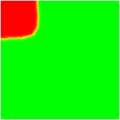
t=240

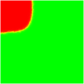
480

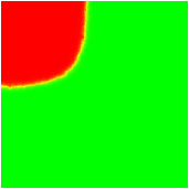
720

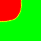
960

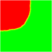
1190

Figure 3: Simulation 1: Parameters as given in (4.2.1.). The first row shows results with white noise, the second row shows spatiotemporally colored noise with $\omega_{ii}=0.03$, $\epsilon=0.001$ and correlation lengths $\tau=1$ and $\lambda=1$.

Then, a biological control measure is applied. The invader population is partly infected and the invasion successfully rolled back.

t=1200

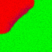
1400

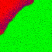
1600

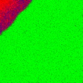
1800

2000

Figure 4: Simulation 1 continued: Partial “blue” infection of the invader at t=1200.

The changes of the fraction of the invaded area can be seen in Figure 5.

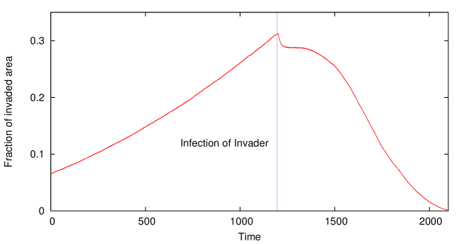
Figure 5: Fraction of invaded area before and after partial infection.

4.2.2. Nonlinear response to noise and noise control of invasion

We now consider the saturating response to noise described above (2.22) with

$$m=n=2\,;\leavevmode\nobreak\ \omega_{11} =50\,,\leavevmode\nobreak\ \omega_{22}=0.1\,,\leavevmode\nobreak\ \omega_{33}=10\,;$$

$$\leavevmode\nobreak\ \gamma_{11} =100\,,\leavevmode\nobreak\ \gamma_{22}=3\,,\leavevmode\nobreak\ \gamma_{33}=300.$$ (4.3)

The extinction of the invader due to hostile environmental conditions is shown in Figure 6. The resident is used and adapted to the environment and happily survives.

t=100

300

400

500

700

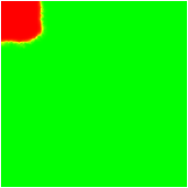
t=500

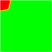
1000

1500

2000

2500

Figure 6: Repressed invasion through population-specific nonlinearly density-dependent noise intensities for white noise in the first row. In the second row for colored noise with correlation lengths $\tau=1$ and $\lambda=1$, $\omega_{11}=0.05$, $\omega_{22}=\omega_{33}=0.01$ qualitatively similar behaviour is observed, albeit on a much slower timescale. However, other simulations have shown that stronger temporal and spatial correlations can support invasions.

This dynamics is only due to the specific noise response of the populations. All growth and interaction parameters remained the same as in sec. 4.2.1.

4.3. Invasions and noise IIa

Coming back to the parameter range of bistability of resident-only state and oscillating coexistence of all three populations, i.e., parameters (4.1.), the initial condition is chosen as uniformly populated by the resident $X_{1}$ at its emergent carrying capacity. At a defined location at the boundary, an initial patch of the invading populations $X_{2}$ and $X_{3}$ attempts to spread. Again, simply linear noise (2.21) is applied and the influence of increasing noise intensity $\omega_{ii}=\omega\,;\leavevmode\nobreak\ i=1,2,3$ ; studied.

It is seen in Figure 7 that a successful invasion requires a certain supercritical noise intensity.

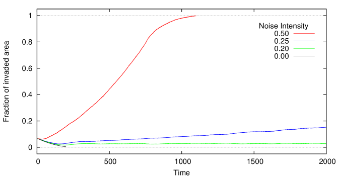
Figure 7: Decline resp. growth of invaded area for increasing white noise intensity.

Somehow, the resident supports the invasion of its own area. Diffusion and noise enhance the mixing of resident and invaders at the front. Therefore, all three together jump on the stable limit cycle of coexistence and invade the remaining invader-free area, cf. Figure 8.

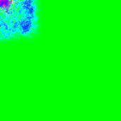
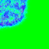
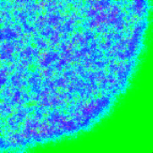
t=0

100

150

350

750

Figure 8: Upper row: Successful fast invasion of the resident’s area for linear white noise (2.21) with $\omega_{ii}=0.5\,;\leavevmode\nobreak\ i=1,2,3$ . Lower row: Stopped invasion of the resident’s area for nonlinear noise (4.2.2.) with $\omega_{ii}=0.25\,;\leavevmode\nobreak\ i=1,2,3\,;\leavevmode\nobreak\ \gamma_{11}=1.00\,,\leavevmode\nobreak\ \gamma_{22}=25.00\,,\leavevmode\nobreak\ \gamma_{33}=4.00$ .

The following Figure 9 shows that weakly correlated noise still allows for invasion but stronger correlated does not.

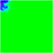
200

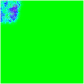
500

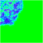
2000

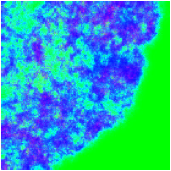
4000

t=0

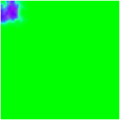
100

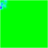
150

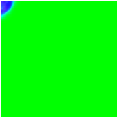
500

1200

Figure 9: Same parameters as in Fig. 8. The invasion is successful for colored noise and correlation lengths $\tau=\lambda=1$ but unsuccessful for $\tau=\lambda=15$. Other parameters $\epsilon=0.001$, $\omega_{ii}=0.05$.

After some difficulties at the beginning that can be the end for the invader at lower noise intensities, the purple invader patch turns into the blue of the limit cycle. Finally, the resident survives but has to share its habitat with the aliens. However, if the nonlinear response or colored noise is applied, the invasion can be stopped and rolled back again.

4.4. Invasions and noise IIb

Now, it is assumed that the limit cycle of resident and invaders has already invaded most of the area and only a small part is left for the resident alone. Again, the parameters (4.1.) are used. For this situation several interesting patterns appear that are again purely due to different properties of the environmental noise.

4.4.1. Dependence on noise intensity

It is surprising that the resident turns out to be strong enough to defeat the invasion as far the noise is below a subcritical threshold. The fraction of invaded area over time is plotted in Figure 10.

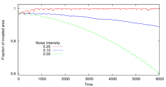
Figure 10: Decline resp. growth of invaded area for increasing white noise intensity.

An example for the defeat of invasion is given in Figure 11.

t=0

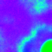
1500

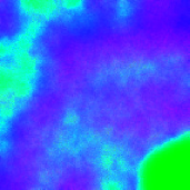
3000

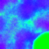
4500

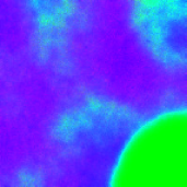
6000

Figure 11: Finally successful defeat of invasion for no noise (upper row) resp. white noise with $\omega_{ii}=0.1\,;\leavevmode\nobreak\ i=1,2,3$.

A preliminary conclusion is that increasing linearly density-dependent white noise supports invasion. In Figure 12, the cloudy result for $\omega_{ii}=0.25$ is shown.

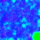
t=100

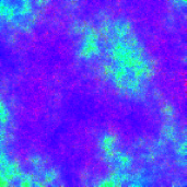
1000

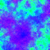
2000

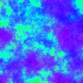
4500

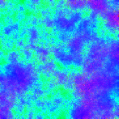
6000

Figure 12: Cloudy invasion for linear white noise with $\omega_{ii}=0.25\,;\leavevmode\nobreak\ i=1,2,3$. Initial condition as in Figure 11.

Increasing the noise intensity and both correlation lengths ($\tau=\lambda=20$) leads to a situation where native and resident gain and lose control over parts of the spatial domain in an alternating fashion (Figure 13). It seems that the resident is slowly getting the upper hand: at $t=7500$ roughly two thirds of the domain are occupied by natives, at $t=10000$ the resident has lost a few areas and displaced the invader in a few others.

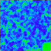
t=50

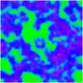
500

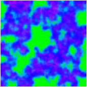
2000

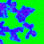
7500

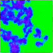
10000

Figure 13: Resident and invader fight under colored noise for territory creating a highly irregular pattern for $\omega_{ii}=0.1\,,\leavevmode\nobreak\ \epsilon=0.001\,,\leavevmode\nobreak\ \tau=20\,,\lambda=20$ . Initial condition as in Figure 11.

4.4.2. Metapopulation patches

This does not necessarily change for nonlinear noise, however, one setting is found where the fraction of invaded area is dropped down from initially 98% to 21%. The resident population splits into three metapopulations, spatially separated by the invader populations, cf. Figure 14.

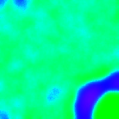
t=500

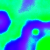
1000

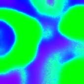
1500

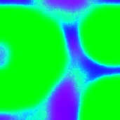
2300

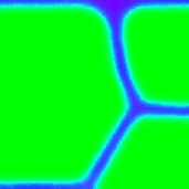
6000

Figure 14: Stable formation of spatially separated patches of the resident population for white noise intensity $\omega_{ii}=0.25\,;\leavevmode\nobreak\ i=1,2,3\,;\leavevmode\nobreak\ \gamma_{11}=1.0\,,\leavevmode\nobreak\ \gamma_{22}=25.0\,,\leavevmode\nobreak\ \gamma_{33}=4.0$ . Initial condition as in Figure 11.

As observed above, higher noise intensities $\omega$ help the invader to establish by stabilising the coexistence limit cycle. In contrast, stronger correlations i.e. increasing correlation lengths $\tau$ in time or $\lambda$ in space generally enable the native species to displace the invaders. Only for relatively high correlation lengths of 10 or above the native species is able to form patches and avoid a cloudy invasion as in Figure 12.

In Figure 15, for a low noise intensity $\omega_{ii}=0.03$, $\tau=1$ and $\lambda=15$ we observe the emergence of a quasi-stationary pattern similar to Figure 14.

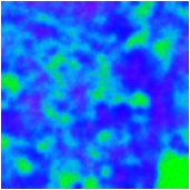
t=340

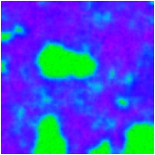
1000

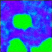
2000

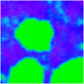
3000

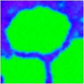
6000

Figure 15: Resident slowly displaces invader while forming seemingly stable spatially separated patches, similar to the results in Figure 14 but without nonlinearity in the noise term. Parameters: $\omega_{ii}=0.03\,,\leavevmode\nobreak\ \epsilon=0.001\,,\leavevmode\nobreak\ \tau=1\,,\lambda=15$ . Initial condition as in Figure 11.

4.4.3. Spiral waves

Wavy structures are found as well, however, at the cost of full invasion. One example is presented in Figure 16.

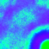
t=500

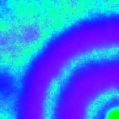
1700

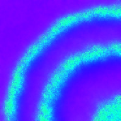
2250

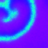
5500

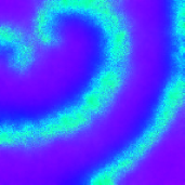
6000

Figure 16: Stable formation of spatially separated patches of the resident population for linear white noise intensity $\omega_{ii}=0.3\,;\leavevmode\nobreak\ i=1,2,3\,;\leavevmode\nobreak\ \gamma_{11}=0.5625\,,\leavevmode\nobreak\ \gamma_{22}=4.0\,,\leavevmode\nobreak\ \gamma_{33}=9.0$ . Initial condition as in Figure 11.

For nonlinear noise, the spiral waves seen in Figure 16 can also be observed if the noise is colored. For small values of spatial and temporal correlation lengths ($\tau=\lambda=1$), smaller and slightly more irregular spiral waves can be observed, cf. Figure 17.

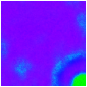
t=1000

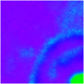
t=2000

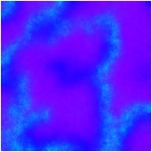
t=5000

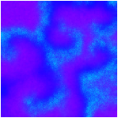
t=7000

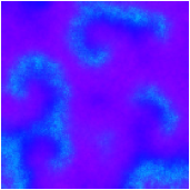
t=9000

Figure 17: Formation of spiral waves – similar to Figure 16 but less regular – for colored noise intensity $\omega_{ii}=0.03\,;\leavevmode\nobreak\ i=1,2,3\,;\leavevmode\nobreak\ \epsilon=0.001\,,\leavevmode\nobreak\ \tau=1\,,\leavevmode\nobreak\ \lambda=1\,,\leavevmode\nobreak\ \gamma_{11}=0.5625\,,\leavevmode\nobreak\ \gamma_{22}=4.0\,,\leavevmode\nobreak\ \gamma_{33}=9.0$ . Initial condition as in Figure 11.

For increased correlation in time or space (e.g. $\tau=1$ as above but $\lambda=5$), the native population can still maintain a spreading front that eventually displaces the spiral waves formed in its wake, cf. Figure 18.

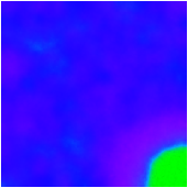
t=1000

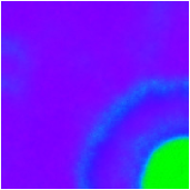
t=2000

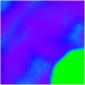
t=5000

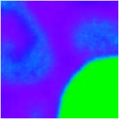
t=7000

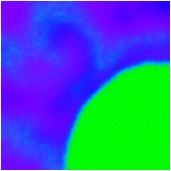
t=9000

Figure 18: For increased spatial correlation the spiral waves are displaced by a front of natives. Parameters: $\omega_{ii}=0.03\,;\leavevmode\nobreak\ i=1,2,3\,;\leavevmode\nobreak\ \epsilon=0.001\,,\leavevmode\nobreak\ \tau=1\,,\leavevmode\nobreak\ \lambda=5,\leavevmode\nobreak\ \gamma_{11}=0.5625\,,\leavevmode\nobreak\ \gamma_{22}=4.0\,,\leavevmode\nobreak\ \gamma_{33}=9.0$ . Initial condition as in Figure 11.

5. Conclusions

Populations are exposed to fluctuations of many environmental parameters such as nutrient availability, temperature etc. that may have positive or adverse effects. Whereas it would be impractical to explicitly consider a host of factors that each on their own may only have a small influence on growth or decline of the population it is possible to represent the collective effect of these factors as stochastic environmental variability. The standard model for stochastic environmental variability in population dynamics are stochastic differential equations with a multiplicative noise term.

In this model, the matrix of maximum noise intensities $\mathbf{\omega}$ is the only parameter that can be used for capturing all aspects of environmental fluctuations. The standard assumption that environmental noise is temporally and spatially uncorrelated neglects the fact that many environmental factors are, in fact, typically correlated.

Whereas at first glance it seems that this can be convincingly justified by assuming that the spatial and temporal correlation lengths $\tau$ and $\lambda$ of the noise are much shorter than the spatiotemporal scale under consideration, we have demonstrated in this study that using correlated instead of uncorrelated noise may lead to qualitatively very different model behaviour. Thus, neglecting possible correlations may, in fact, lead to different explanations of the observed system behaviour.

Another implicit assumption that has previously been unquestioned is the linear increase of noise intensity with population number. This model implies that environmental effects on each individual in a population simply add up to an overall effect on the population. In our opinion it is likely that for increasing population numbers, perturbations should not independently affect each individual but rather saturate due to interactions of the individuals so that the collective response of the population saturates to a maximum noise intensity for large population numbers. This model requires an additional matrix $\mathbf{\gamma}$ which characterises the ability of the population to “buffer” stochastic fluctuations: for low values of $\gamma_{ii}$, population $X_{i}$ is exposed to intensities close to the maximum noise level $\omega_{ii}$ for low or moderate population numbers whereas for a population with a large $\gamma_{ii}$ the noise intensity $\omega_{ii}$ is only reached for high population numbers.

The results presented in this paper have been obtained for purely diagonal noise intensity matrices. More complex forms are left to future work.

Acknowledgements

H.M. did most of the work on this paper during a semi-sabbatical in Brazil, France and Japan. He acknowledges substantial financial support by the Coordenação de Aperfeiçoamento de Pessoal de Nível Superior (CAPES, Brazil), the Fundação de Amparo à Pesquisa do Estado do Rio Grande do Sul (FAPERGS, Brazil), the Initiative d’Excellence de l’Université de Bordeaux (IdEX Bordeaux, France), the Japan Society for the Promotion of Science (JSPS, Japan) and last but not least by the Deutscher Akademischer Austauschdienst (DAAD, Germany). And he very much appreciated the scientific expertise and warm hospitality of the host working groups at Santa Maria RS, Bordeaux and Osaka.

References

- [1] R. M. Anderson, R. M. May. The invasion, persistence and spread of infectious diseases within animal and plant communities. Philosophical Transactions of the Royal Society of London B, 314 (1986), 533–570.
- [2] S. Bedhomme, P. Agnew, Y. Vital, C. Sidobre, Y. Michalakis. Prevalence-dependent costs of parasite virulence. PLoS Biology, 3 (2005), e262.
- [3] G. E. P. Box, M. E. Muller. A note on the generation of random normal deviates. Annals of Mathematical Statistics, 29 (1958), no. 2, 610–611.
- [4] J.-B. Burie, A. Calonnec, M. Langlais. Modeling of the invasion of a fungal disease over a vineyard. In A. Deutsch, R. B. de la Parra, R. J. de Boer, O. Diekmann, P. Jagers, E. Kisdi, M. Kretzschmar, P. Lansky, H. Metz (Eds.), Mathematical Modeling of Biological Systems, Volume II. Epidemiology, Evolution and Ecology, Immunology, Neural Systems and the Brain, and Innovative Mathematical Methods, Modeling and Simulation in Science, Engineering and Technology. Birkhäuser, Boston, 2008, pages 11–21.
- [5] E. M. Coombs, J. K. Clark, G. L. Piper, A. F. Cofrancesco Jr. (Eds.). Biological control of invasive plants in the United States. Oregon State University Press, Corvallis OR, 2004.
- [6] J. A. Drake, H. A. Mooney (Eds.). Biological invasions: a global perspective, vol. 27 of SCOPE. Wiley, Chichester, 1989.
- [7] H. I. Freedman. A model of predator-prey dynamics as modified by the action of a parasite. Mathematical Biosciences, 99 (1990), 143–155.
- [8] J. S. Fulda. The logistic equation and population decline. Journal of Theoretical Biology, 91 (1981), 255–259.
- [9] L. Q. Gao, H. W. Hethcote. Disease transmission models with density dependent demographics. Journal of Mathematical Biology, 30 (1992), 717–731.
- [10] D. García-Álvarez. A comparison of a few numerical schemes for the integration of stochastic differential equations in the Stratonovich interpretation. arXiv:1102.4401v1 [physics.comp-ph], (2011).
- [11] J. García-Ojalvo, J. M. Sancho. Noise in spatially extended systems. Institute for Nonlinear Science. Springer, New York, 1999.
- [12] J. García-Ojalvo, J. M. Sancho, L.Ramírez-Piscina. Generation of spatiotemporal colored noise. Physical Review E, 46 (1992), no. 8, 4670–4675.
- [13] K. P. Hadeler, H. I. Freedman. Predator-prey populations with parasitic infection. Journal of Mathematical Biology, 27 (1989), 609–631.
- [14] K. Harley, I. W. Forno. Biological control of weeds: a handbook for practitioners and students. Inkata Press, Melbourne, 1992.
- [15] R. Hengeveld (Ed.). Dynamics of biological invasions. Chapman and Hall, London, 1989.
- [16] F. M. Hilker, H. Malchow. Strange periodic attractors in a prey-predator system with infected prey. Mathematical Population Studies, 13 (2006), no. 3, 119–134.
- [17] K. Itó. On stochastic differential equations. Memoirs of the American Mathematical Society, 4 (1951), 1–51.
- [18] R. Jarrow, P. Protter. A short history of stochastic integration and mathematical finance: the early years, 1880–1970. In Anirban DasGupta (Ed.), A Festschrift for Herman Rubin, vol. 45 of Lecture Notes – Monograph Series. Institute of Mathematical Statistics, Beachwood, Ohio, USA, 2004, pages 75–91.
- [19] M. Julien, G. White (Eds.). Biological control of weeds: theory and practical application. No. 49 in ACIAR Monograph Series. Australian Centre for International Agricultural Research, Bruce ACT, 1997.
- [20] N. Keiding. Extinction and exponential growth in random environments. Theoretical Population Biology, 8 (1975), no. 1, 49 – 63.
- [21] P. E. Kloeden, E. Platen. Numerical solution of stochastic differential equations, vol. 23 of Applications of Mathematics. Springer, Berlin, 1999.
- [22] E. Kuno. Some strange properties of the logistic equation defined with r and K: Inherent effects or artefacts? Researches on Population Ecology, 33 (1991), 33–39.
- [23] T. G. Kurtz. Diffusion approximations for branching processes. In A. Joffe, P. Ney (Eds.), Branching processes, vol. 5 of Advances in Probability and Related Topics. Marcel Dekker, New York – Basel, 1978, pages 269–292.
- [24] V. Lehmann. Invasion, Konkurrenz und Kontrolle einer fremden Art. Diplomarbeit, Institut für Umweltsystemforschung, Fachbereich Mathematik/Informatik, Universität Osnabrück (2011).
- [25] H. Malchow, A. James, R. Brown. Competitive and diffusive invasion in a noisy environment. Mathematical Medicine and Biology, 28 (2011), 153–163. doi:10.1093/imammb/dqq008.
- [26] H. Malchow, A. James, R. Brown. Control of competitive bioinvasion. In M. E. Lewis, P. K. Maini, S. V. Petrovskii (Eds.), Dispersal, individual movement and spatial ecology: A mathematical perspective, vol. 2071 of Lecture Notes in Mathematics. Springer, Berlin, 2013, pages 293–305.
- [27] H. Malchow, L. Schimansky-Geier. Noise and diffusion in bistable nonequilibrium systems, vol. 5 of Teubner-Texte zur Physik. Teubner-Verlag, Leipzig, 1985.
- [28] J. Mallet. The struggle for existence: how the notion of carrying capacity, K, obscures the links between demography, Darwinian evolution, and speciation. Evolutionary Ecology Research, 14 (2012), 627–665.
- [29] M. Matsumoto, T. Nishimura. Mersenne Twister: a 623-dimensionally equidistributed uniform pseudorandom number generator. ACM Transactions on Modeling and Computer Simulation, 8 (1998), no. 1, 3–30.
- [30] R. M. May. Stability and complexity in model ecosystems, vol. 6 of Monographs in Population Biology. Princeton University Press, Princeton, 1973.
- [31] R. M. May. Stability in randomly fluctuating versus deterministic environments. The American Naturalist, 107 (1973), no. 957, 621–650.
- [32] H. McCallum, N. Barlow, J. Hone. How should pathogen transmission be modelled? Trends in Ecology & Evolution, 16 (2001), no. 6, 295–300.
- [33] P. B. McEvoy, E. M. Coombs. Biological control of plant invaders: Regional patterns, field experiments, and structured population models. Ecological Applications, 9 (1999), no. 2, 387–401.
- [34] P.-A. Meyer. Stochastic processes from 1950 to the present. Electronic Journal for History of Probability and Statistics, 5 (2009), no. 1, 1–42.
- [35] G. N. Milstein. Chislennoe integrirovanie stokhasticheskikh differentsial’nykh uravnenii. Izdatel’stvo Ural’skogo Universiteta, Sverdlovsk, 1988.
- [36] G. N. Milstein. Numerical integration of stochastic differential equations, vol. 313 of Mathematics and Its Applications. Kluwer Academic Publishers, Dordrecht, 1995.
- [37] D. Mollison. Modelling biological invasions: chance, explanation, prediction. Philosophical Transactions of the Royal Society of London B, 314 (1986), 675–693.
- [38] C. Mueller. Some tools and results for parabolic stochastic partial differential equations. In D. Khoshnevisan, F. Rassoul-Agha (Eds.), A minicourse on stochastic partial differential equations, vol. 1962 of Lecture Notes in Mathematics, chap. 4. Springer, Berlin, Heidelberg, 2009, pages 111–144.
- [39] A. Nitzan, P. Ortoleva, J. Ross. Nucleation in systems with multiple stationary states. Faraday Symposia of the Chemical Society, 9 (1974), 241–253.
- [40] D. W. Peaceman, H. H. Rachford Jr. The numerical solution of parabolic and elliptic differential equations. Journal of the Society for Industrial and Applied Mathematics, 3 (1955), 28–41.
- [41] D. Pimentel (Ed.). Biological invasions. Economic and environmental costs of alien plant, animal, and microbe species. CRC Press, Boca Raton, 2002.
- [42] J. Ripa, P. Lundberg, V. Kaitala. A general theory of environmental noise in ecological food webs. American Naturalist, 151 (1998), 256–263.
- [43] D. F. Sax, J. J. Stachowicz, S. D. Gaines (Eds.). Species invasions. Insights into ecology, evolution, and biogeography. Sinauer, Sunderland, 2005.
- [44] T. Schaffter. Numerical integration of SDEs: a short tutorial (2010). Laboratory of Intelligent Systems, Swiss Federal Institute of Technology at Lausanne (EPFL), Switzerland.
- [45] N. Shigesada, K. Kawasaki. Biological invasions: Theory and practice. Oxford University Press, Oxford, 1997.
- [46] M. Sieber, H. Malchow, F. M. Hilker. Disease-induced modification of prey competition in eco-epidemiological models. Ecological Complexity, 18 (2014), 74–82.
- [47] I. Siekmann. Mathematical modelling of pathogen-prey-predator interactions. Verlag Dr. Hut, München, 2009.
- [48] I. Siekmann. On competition in ecology, epidemiology and eco-epidemiology. Ecological Complexity, 14 (2013), 166–179.
- [49] W. L. Smith. Necessary conditions for almost sure extinction of a branching process with random environment. Annals of Mathematical Statistics, 39 (1968), no. 6, 2136–2140.
- [50] W. L. Smith, W. E. Wilkinson. On branching processes in random environments. Annals of Mathematical Statistics, 40 (1969), no. 3, 814–827.
- [51] R. L. Stratonovich. Topics in the theory of random noise, vol. 3 (1 & 2) of Mathematics and Its Applications. Gordon and Breach, New York, 1963 & 1967.
- [52] J. W. Thomas. Numerical partial differential equations: Finite difference methods, vol. 22 of Texts in Applied Mathematics. Springer, New York, 1995.
- [53] P. van den Driessche, M. L. Zeeman. Disease induced sscillations between two competing species. SIAM Journal of Applied Dynamical Systems, 3 (2004), no. 4, 601–619.
- [54] J. E. van der Plank. Host-pathogen interactions in plant disease. Academic Press, New York, 1982.
- [55] E. Venturino. The influence of diseases on Lotka-Volterra systems. IMA Preprint Series 913, Institute of Mathematics and its Applications, University of Minnesota, Minneapolis (1992).
- [56] E. Venturino. The influence of diseases on Lotka-Volterra systems. Rocky Mountain Journal of Mathematics, 24 (1994), 381–402.
- [57] E. Venturino. The effect of diseases on competing species. Mathematical Biosciences, 174 (2001), 111–131.
- [58] J. B. Walsh. An introduction to stochastic partial differential equations. In R. Carmona, H. Kesten, J. B. Walsh (Eds.), École d’été de probabilités de Saint-Flour XIV - 1984, vol. 1180 of Lecture Notes in Mathematics. Springer, Berlin, 1986, pages 265–437.
- [59] M. Williamson. Biological invasions, vol. 15 of Population and Community Biology Series. Chapman & Hall, London, 1996.
- [60] T. Woyzichovski. Der Einfluss von Rauschen und Infektion in einem Konkurrenzmodell fremder und indigener Spezies. Diplomarbeit, Institut für Umweltsystemforschung, Fachbereich Mathematik/Informatik, Universität Osnabrück (2013).