Homogeneous solutions for elliptically polarized light in a cavity containing materials with electric and magnetic nonlinearities

Abstract

We study evolution equations and stationary homogeneous solutions for electric and magnetic field amplitudes in a ring cavity with flat mirrors. The cavity is filled with a positive or negative refraction index material with third order Kerr-like electric nonlinearities and also magnetic nonlinearities, which can be relevant in metamaterials. We consider the degree of freedom of polarization in the incident beam. It is found that considering a magnetic nonlinearity increases the variety of possible qualitatively different solutions. A classification of solutions is proposed in terms of the number of bifurcations. The analysis can be useful for the implementation of optical switching or memory storage using ring cavities with non linear materials.

PACS: 05.45.-a, 42.65.Hw, 42.70.Mp

I Introduction

During the last decade, progress in the development of composite materials allowed the experimental observation of new optical properties, such as negative refraction index smith ; shelby . These materials have both negative dielectric permittivity and negative magnetic permeability, a property not found in natural materials. Materials with negative refraction index (NRM) have many interesting new features, and a great number of applications have been proposed based on their novel properties.

On the other hand, ring cavities filled with nonlinear media have been proposed for information storage and also as the optical analog of electrical transistors moloney . Conditions for modifying and tuning optical bistability in these cavities are being researched Kim ; anton . It is known that electromagnetic wave propagation in a Kerr-type nonlinear material with a positive refraction index (PRM) can be described by an order parameter equation of the nonlinear Schrödinger type and the same type of equation can be extended to NRM kockaert ; kockaert2 ; wen ; scalora ; lazarides .

A recent work Merlin shows that arguments previously used to neglect the magnetic response in a PRM do not hold for NRM, where both the polarization and the magnetization may take non-negligible values. Even, it has been shown zharov ; lapine that a composite metamaterial with negative refraction index could develop a nonlinear macroscopic magnetic response. This means that although the medium has a negligible magnetic nonlinearity, periodic inclusions produce a nonlinear effective response when the wavelength is much larger than the periodicity of the inclusions.

In this paper we analyze the equations describing the electric and magnetic fields in a ring cavity with flat mirrors that contains a NRM or a PRM with electric and magnetic nonlinearities. In a previous work nosotros , we limited ourselves to a linearly polarized incident beam, now we focus on analyzing what happens when the light polarization is taken into account, making it necessary the double of equations to describe the system. The main objective of this paper is to explore the various types of stationary homogeneous solutions that the system can display, depending on the parameters that describe it. We also perform a brief analysis of the behavior of linearly unstable solutions.

The paper is organized as follows. In section II we present the evolution equations for the amplitude of the electric and magnetic fields and the reduction to two coupled Lugiato Lefever equations for a ring cavity. In section III we analyze homogeneous stationary solutions. The type and number of bifurcations that can occur, depending on the parameters, are also analyzed. Finally, in section IV, numerical integration is performed in order to analyze the temporal evolution of the unstable solutions. In section V we present our conclusions.

II Cavity Equations

The equations often used for describing the behavior of electric and magnetic fields, at the plane perpendicular to propagation of light in a cavity, are of the type of Lugiato-Lefever equation (LL, see lugiato ) with generalized parameters. LL equation is a simple mean field model, and has been useful for the analysis of pattern formation in cavities containing a Kerr medium that is driven by a coherent plane wave hoyuelos ; firth .

First, we analyze the problem of free propagation (without mirrors) of an electromagnetic wave in a nonlinear material, either PRM or NRM, and then we use the resulting equations to obtain the behavior in the cavity.

II.1 Evolution Equations in the material

We consider a plane wave of arbitrary polarization and frequency $\omega_{0}$. We assume that the electric and magnetic fields are in the plane $x$-$y$ and the wave propagates in the $z$ axis. The starting point is Maxwell’s equations and constitutive relations for the electric displacement, $\mathbf{D}=\epsilon_{0}\mathbf{E}+\mathbf{P}$, and magnetic induction, $\mathbf{B}=\mu_{0}\mathbf{H}+\mu_{0}\mathbf{M}$. An isotropic metamaterial is analyzed with the third-order Kerr nonlinear response. The nonlinear relationship between the polarization of the material and the electric field is moloney :

$$P_{i}(t) = \epsilon_{0}\int_{-\infty}^{\infty}\chi^{(1)}_{E,ij}(t-\tau)\,E_{j}(\tau)\,d\tau$$ (1)

$$+\epsilon_{0}\int_{-\infty}^{\infty}\chi^{(3)}_{E,ijkl}(t-\tau_{1},t-\tau_{2},t-\tau_{3})\,E_{j}(\tau_{1})E_{k}(\tau_{2})E_{l}(\tau_{3})\,d\tau_{1}d\tau_{2}d\tau_{3},$$

where $i,j,k$ and $l$ correspond to Cartesian axes, and take values $x$, $y$ or $z$; repeated indexes involve addition. $\chi^{(1)}_{E,ij}$ is a rank 2 tensor describing linear electric behavior in the material and $\chi^{(3)}_{E,ijkl}$ accounts for third order nonlinearities.

Zharov et al zharov analyzed properties of a microstructured metamaterial made of metallic wires and split ring resonators (SRR) embedded into a Kerr permittivity material. They found out that, in such a material, the electric fields around the SRR could be very strong. In that case, the electric nonlinearity produces an effective magnetic nonlinearity $\mu_{eff}$. Expanding $\mu_{eff}$ in powers of the incident magnetic field, to the lowest non constant order, a Kerr-like magnetization can be found. Thus, a similar relationship to (1) is proposed for magnetization and magnetic field (with similar definitions for $\chi^{(1)}_{M}$ and $\chi^{(3)}_{M}$):

$$M_{i}(t) = \int_{-\infty}^{\infty}\chi^{(1)}_{M,ij}(t-\tau)\,H_{j}(\tau)\,d\tau$$ (2)

$$+\int_{-\infty}^{\infty}\chi^{(3)}_{M,ijkl}(t-\tau_{1},t-\tau_{2},t-\tau_{3})\,H_{j}(\tau_{1})H_{k}(\tau_{2})H_{l}(\tau_{3})\,d\tau_{1}d\tau_{2}d\tau_{3}.$$

Many proposed metamaterials consist of the repetition of a cubic unit lattice which has the same form when it is looked from any of its faces (for example, materials using spherical inclusions Holloway , spherical inclusions and wires Cai but also cells specifically designed to be symmetric Koschny ), making optical properties to be the same in any two orthogonal directions. If the wavelength of incident light is much larger than the cell length, the material is expected to be isotropic. So, we assume that the material is cubic centrosymmetric and isotropic. As the components of the tensors $\chi^{(3)}_{E/M}$ take part only on field convolutions, the tensors are defined, without loss of generality, to be symmetrical for a large number of indexes and argument permutations, similar to what has been done in moloney , Ch. 2, Sect. 2d.

We apply the classical multiple scales perturbation technique, and we assume that light is quasi-monochromatic and can be represented by a plane wave, with frequency $\omega_{0}$ and wavenumber $k_{0}$. It travels thought the $z$ axis, and is modulated by a slowly varying amplitude. The amplitude depends on position $\mathbf{R}=(X,Y,Z)$ and time $T$, variables that have characteristic scales much larger than the scales given by $1/k_{0}$ and $1/\omega_{0}$. In summary, the fields $\mathbf{E}$ and $\mathbf{H}$ can written as

$$\mathbf{E} = \boldsymbol{\mathcal{E}}(\mathbf{R},T)e^{i(k_{0}z-\omega_{0}t)}+c.c.$$

$$\mathbf{H} = \boldsymbol{\mathcal{H}}(\mathbf{R},T)e^{i(k_{0}z-\omega_{0}t)}+c.c.$$ (3)

where $\boldsymbol{\mathcal{E}}$ and $\boldsymbol{\mathcal{H}}$ are slowly varying amplitudes. Similar relationships are defined for $P$ and $M$; the corresponding amplitudes can be written as (for the polarization of material see, for example, geddes )

$$\boldsymbol{\mathcal{P}} = 3\chi^{(3)}_{E}\left[A_{E}(|\mathcal{E}_{x}|^{2}+|\mathcal{E}_{y}|^{2})\boldsymbol{\mathcal{E}}+B_{E}/2(\mathcal{E}_{y}^{2}+\mathcal{E}_{x}^{2})\bar{\boldsymbol{\mathcal{E}}}\right]$$

$$\boldsymbol{\mathcal{M}} = 3\chi^{(3)}_{M}\left[A_{M}(|\mathcal{H}_{x}|^{2}+|\mathcal{H}_{y}|^{2})\boldsymbol{\mathcal{H}}+B_{M}/2(\mathcal{H}_{y}^{2}+\mathcal{H}_{x}^{2})\bar{\boldsymbol{\mathcal{H}}}\right],$$ (4)

where the bar stands for complex conjugate, $\chi^{(3)}_{E/M}=\chi^{(3)}_{E/M,xxxx}$ and parameters $A_{E/M}$ and $B_{E/M}$ are given by

$$A_{E/M} = \frac{\chi^{(3)}_{E/M,yyxx}+\chi^{(3)}_{E/M,yxyx}}{\chi^{(3)}_{E/M}}$$

$$B_{E/M} = 2\frac{\chi^{(3)}_{E/M,yxxy}}{\chi^{(3)}_{E/M}}.$$ (5)

In the previous expressions we are using the notation $\chi^{(3)}_{E/M,abcd}$ (without explicit dependence) to identify the Fourier transform of $\chi^{(3)}_{E/M,abcd}(t_{1},t_{2},t_{3})$ evaluated in $(\omega_{0},\omega_{0},-\omega_{0})$.

We define the wavenumber $k(\omega)=\omega n(\omega)/c$; $k^{\prime}$ and $k^{\prime\prime}$ are the derivatives of $k(\omega)$ at $\omega=\omega_{0}$; the refraction index is $n(\omega)=\pm\sqrt{\epsilon_{r}(\omega)\,\mu_{r}(\omega)}$ (which takes a negative value when both $\epsilon_{r}$ and $\mu_{r}$ are negative veselago ), where $\epsilon_{r}(\omega)=1+\chi^{(1)}_{E}(\omega)$ and $\mu_{r}(\omega)=1+\chi^{(1)}_{M}(\omega)$ are the relative permittivity and relative permeability, respectively.

The details of the implementation of multiple scales technique in our case, are essentially the same as those described in reference moloney , Sect. 2k. After this process, we obtain nonlinear Schrödinger equations for the envelopes of electric and magnetic fields defined in the plane perpendicular to the $z$ axis. Applying a change of variables to use circularly polarized components, $\sqrt{2}\mathcal{E}_{\pm}=\mathcal{E}_{x}\pm i\mathcal{E}_{y}$, $\sqrt{2}\mathcal{H}_{\pm}=\mathcal{H}_{y}\mp i\mathcal{H}_{x}$, and a coordinate transformation given by $\xi=z$, $\tau=t-k^{\prime}z$, the following equations of evolution in the material can be found

$${\partial\mathcal{E}_{\pm}\over\partial\xi} = -k^{\prime\prime}(\omega_{0}){i\over 2}{\partial^{2}\mathcal{E}_{\pm}\over\partial t^{2}}+{i\over 2k_{0}}\nabla_{\perp}^{2}\mathcal{E}_{\pm}+{3k_{0}i\over 2}\left[{\chi^{(3)}_{E}\over\varepsilon_{r}}(A_{E}|\mathcal{E}_{\pm}|^{2}+(A_{E}+B_{E})|\mathcal{E}_{\mp}|^{2})\right.$$ (6)

$$\left.+{\chi^{(3)}_{M}\over\mu_{r}}(A_{M}|\mathcal{H}_{\pm}|^{2}+(A_{M}+B_{M})|\mathcal{H}_{\mp}|^{2})\right]\mathcal{E}_{\pm}$$

$${\partial\mathcal{H}_{\pm}\over\partial\xi} = -k^{\prime\prime}(\omega_{0}){i\over 2}{\partial^{2}\mathcal{H}_{\pm}\over\partial t^{2}}+{i\over 2k_{0}}\nabla_{\perp}^{2}\mathcal{H}_{\pm}+{3k_{0}i\over 2}\left[{\chi^{(3)}_{E}\over\varepsilon_{r}}(A_{E}|\mathcal{E}_{\pm}|^{2}+(A_{E}+B_{E})|\mathcal{E}_{\mp}|^{2})\right.$$ (7)

$$\left.+{\chi^{(3)}_{M}\over\mu_{r}}(A_{M}|\mathcal{H}_{\pm}|^{2}+(A_{M}+B_{M})|\mathcal{H}_{\mp}|^{2})\right]\mathcal{H}_{\pm}$$

where the approximation $k_{0}^{2}\simeq\omega_{0}^{2}\mu_{0}\mu_{r}\varepsilon_{0}\varepsilon_{r}$, valid for low dispersion fields, is used. For simplicity of notation we write $\mu_{r}(\omega_{0})=\mu_{r}$ and $\varepsilon_{r}(\omega_{0})=\varepsilon_{r}$.

Linear and nonlinear dissipation is neglected, so that $\chi^{(1)}_{E/M}$ and $\chi^{(3)}_{E/M}$ are real valued quantities. This is an often used approach in conventional optics, but dissipation could play an important role in metamaterials. Nevertheless, as we comment in the next section, there are ways to reduce dissipation in metamaterials even to negligible levels. On the other hand, a generalization of the model for small dissipation is also possible nosotros .

II.2 Cavity effects

Figure 1: Scheme of the ring cavity.

We consider a ring cavity with plane mirrors and with a nonlinear material as shown in Figure 1. At the input mirror, the incident fields are $E_{\mathrm{in}}$ and $H_{\mathrm{in}}$, and the reflection and transmission coefficient are $r_{i}$ and $t_{i}$ respectively; $T_{r}$ is the round trip time and $L$ is the nonlinear material length. The detuning between the incident field and the cavity mode is $\theta=\phi\mod 2\pi$ where $\phi$ is the phase accumulated by the wave around the cavity, including the effects of reflections in the mirrors. We study the cavity near resonance, so the mismatch is small and $e^{i\theta}\simeq 1+i\theta$.

From Maxwell equations, assuming that nonlinearities are small, it is obtained that, in a given medium (different from vacuum), the relationship between electric and magnetic fields is approximately $\mathcal{H}_{\pm}=\eta\mathcal{E}_{\pm}$ while in vacuum the relation is $\mathcal{H}_{\pm}=\eta_{0}\mathcal{E}_{\pm}$, where $\eta$ and $\eta_{0}$ are the inverses of the material and vacuum impedances, respectively. If we consider media with similar impedances ($\eta\simeq\eta_{0}$), the wave is mainly transmitted, generating a negligible reflected wave . The transmitivity coefficients at both ends of the material are $t_{\pm}=1\pm{\eta_{m}-\eta_{0}\over\eta_{m}+\eta_{0}}$, where $t_{+}$ holds for $\mathcal{E}$ at point $b$ (see Fig. 1) and for $\mathcal{H}$ at point $a$, and $t_{-}$ holds for $\mathcal{H}$ at $b$ and for $\mathcal{E}$ at $a$.

We can obtain an equation of evolution for electric and magnetic fields in the cavity and it can be shown that under the above conditions, the proportionality between them is maintained, so the system is well described knowing only the electric field. The procedure is analogous to that performed in nosotros . It is important to mention that from now on we are looking at cases where transverse spatial dependence can be neglected, i.e. $\nabla_{\perp}^{2}\mathcal{E}_{\pm}\simeq 0$. We get

$$T_{r}{\partial\mathcal{E}_{\pm}\over\partial t} = t_{i}E_{in\pm}+(\rho-1+\rho i\theta)\mathcal{E}_{\pm}+{3\rho iLk_{0}\over 2\varepsilon_{r}}\left[(t_{+}^{2}\eta^{2}\chi^{(3)}_{M}B_{M}+t_{-}^{2}\chi^{(3)}_{E}B_{E})|\mathcal{E}_{\mp}|^{2}\right.$$ (8)

$$\left.+(t_{+}^{2}\eta^{2}\chi^{(3)}_{M}A_{M}+t_{-}^{2}\chi^{(3)}_{E}A_{E})(|\mathcal{E}_{+}|^{2}+|\mathcal{E}_{-}|^{2})\right]\mathcal{E}_{\pm}.$$

In order to reduce the number of parameters, an equation with adimensional quantities can be obtained using the following change of variables

$$t^{\prime}={t(1-\rho)\over T_{r}} \Theta={-\rho\theta\over(1-\rho)}$$ (9)

$$A_{\pm}={\mathcal{E}_{\pm}\over\mathcal{E}_{t}}\sqrt{Lk_{0}\rho\over 2\varepsilon_{r}(1-\rho)} A_{in\pm}={t_{i}E_{in\pm}\over\mathcal{E}_{t}(1-\rho)}\sqrt{Lk_{0}\rho\over 2\varepsilon_{r}(1-\rho)}$$ (10)

where $\rho=r_{i}t_{+}t_{-}\lesssim 1$ so that $1-\rho$ is a small number of the order of $\theta$, and $\mathcal{E}_{t}$ is a characteristic field given by $1/\sqrt{|3\chi^{(3)}_{M}t_{+}^{2}\eta^{2}+3\chi^{(3)}_{E}t_{-}^{2}|}$.  It is useful to define the parameter $\bar{B}$ as

$$\bar{B}={\eta^{2}\chi^{(3)}_{M}t_{+}^{2}B_{M}+\chi^{(3)}_{E}t_{-}^{2}B_{E}\over\eta^{2}\chi^{(3)}_{M}t_{+}^{2}+\chi^{(3)}_{E}t_{-}^{2}}$$ (11)

that can be understood as an average of the electric and magnetic constants $B_{E}$ and $B_{M}$. In the general case, using symmetry arguments, it can be shown that $A_{E}+B_{E}/2=A_{M}+B_{M}/2=1$. In Ref. boyd (see p. 197), three possible cases are mentioned for only electric nonlinearities (i.e. $A_{M}=B_{M}=0$): $B_{E}=0$ ($\bar{B}=0$), for electrostriction, that does not act at optical frequencies; $B_{E}=6A_{E}$ ($\bar{B}=3/2$) for molecular orientation effects; and $B_{E}=A_{E}$ ($\bar{B}=2/3$) in materials with electronic response far from resonance frequency. In the rest of our work, we will find analytical results for any value of $\bar{B}$, but we will limit our numerical results to the case $0\leq\bar{B}\leq 2$, which corresponds to situations in which $A_{E/M}\geq 0$, and where $\chi_{E}^{(3)}$ has the same sign as $\chi_{E}^{(3)}$. The motivation of the last choice is a result of Ref. zharov , where the authors derive an effective Kerr-like nonlinear magnetization for a split ring resonator; it can be written as $\mu_{\mathrm{eff}}=\mu_{\mathrm{eff}0}+KH^{2}$, where $K$ is a complex number related to geometrical factors, which tends to a real quantity with the same sign as the electric nonlinearity, when conductivity tends to $\infty$. Eq. (8) finally reads:

$${\partial A_{\pm}\over\partial t^{\prime}}=A_{in\pm}-(1+i\Theta)A_{\pm}+i\alpha(|A_{\pm}|^{2}(1-\bar{B}/2)+|A_{\mp}|^{2}(1+\bar{B}/2))A_{\pm},$$ (12)

where $\alpha$ is the sign of $\chi^{(3)}_{M}t_{+}^{2}\eta^{2}+\chi^{(3)}_{E}t_{-}^{2}$. Let us note that dispersion effects, proportional to $k^{\prime\prime}$, are not included, neither in Eq. (8) nor in Eq. (12). The reason is that dispersion generates a term in (12) proportional to the small parameter $1-\rho$ used in the scaling (9) and (10), so that it can be neglected with respect to the other terms.

Considering transverse spatial effects would produce the inclusion of a Laplacian in Eqs. (12), transforming them into Lugiato Lefever equations. Complex conjugate fields describe the same physical system and the corresponding equation is equal to (12) with $\Theta$ and $\alpha$ with opposite signs, therefore the relevant parameter is $\alpha\Theta$. Considering a metamaterial in this analysis justifies the inclusion of the magnetic nonlinearity, that allows a wider range of possible values of $\bar{B}$. The sign of the refraction index does not appear explicitly in (12), but it would appear in a diffraction term if we would take into account transverse spatial effects nosotros .

Up to now, losses have not been taken into account. In the Gigahertz range, it is possible to build an NRM with small (and even negligible) imaginary parts of $\epsilon_{r}$ and $\mu_{r}$ as was shown in, for example, liu ; wang , but for higher frequencies the former is not true. Many proposals for reducing losses at high frequencies are being researched, such as dolling ; shalaev ; popov . If dissipation is not strong, Eq. (12) can be generalized in a similar way to what has been done in a previous work nosotros . Taking $k(\omega_{0})=k_{0}+ik_{I}$, if $k_{I}\ll k_{0}$, the term $-k_{I}\mathcal{E_{\pm}}$ has to be added to the right hand side of equation (6), $-k_{I}\mathcal{H_{\pm}}$ has to be added to the right hand side of equation (7) and $-Lk_{I}\mathcal{E_{\pm}}$ has to be added to the right hand side of equation (8). An adequate change of variables is easily found replacing $(1-\rho)$ by $(1-\rho+\rho Lk_{I})$ in (9) and (10), so that (12) is still valid.

III Homogeneous Stationary Solutions

Looking for stationary homogeneous solutions in (12), we obtain

$$A_{in\pm}=[1+i\Theta-i\alpha(1-\bar{B}/2)|A_{\pm}|^{2}-i\alpha(1+\bar{B}/2)|A_{\mp}|^{2}]A_{\pm}.$$ (13)

From this equation, using that $\alpha^{2}=1$ we can write

$$\lambda I_{in} = \left(1+[\alpha\Theta-(1-\bar{B}/2)I_{+}-(1+\bar{B}/2)I_{-}]^{2}\right)I_{+}$$

$$(1-\lambda)I_{in} = \left(1+[\alpha\Theta-(1-\bar{B}/2)I_{-}-(1+\bar{B}/2)I_{+}]^{2}\right)I_{-}$$ (14)

where $I_{\pm}=|A_{\pm}|^{2}$, $I_{in}=|A_{in+}|^{2}+|A_{in-}|^{2}$, and $\lambda=|A_{in+}|^{2}/I_{in}$ is a quantity that measures the polarization of the incident beam, related to the ellipticity $\chi$ by $\lambda=\cos^{2}(\chi/2)$.

Given a set of parameters ($\alpha\Theta,\bar{B},\lambda$), solution sets $(I_{in},I_{+},I_{-})$ can be obtained. By definition, $0\leq\lambda\leq 1$, but, for each solution with $\lambda>1/2$ there is another solution that can be found exchanging $\mathcal{E}_{+}$ with $\mathcal{E}_{-}$, so, we work with $1/2\leq\lambda\leq 1$.

It was found that the type of possible solutions varies according to the parameters of the system. We present a list of them for linear, circular and elliptic polarization.

III.1 Linear polarization, $\lambda=1/2$

An analysis of Eq. (III) indicates that the symmetric solution ($I_{+}=I_{-}$) always exists, but there may be more solutions. We found, in terms of bifurcations of intensity, a total of 8 possible cases. These 8 possible cases define, in the $\alpha\Theta$-$\bar{B}$ plane, 8 regions, that are limited by 4 curves, as shown in Figure 2(a).

The symmetric solution (regardless if asymmetric solutions exist or not) presents bistability if $\alpha\Theta>\sqrt{3}$, independently of $\bar{B}$. The bistability region (i.e. the range of values of $I_{in}$ for which there are two stable solutions of $I_{\pm}$ ) is limited by a pair of saddle-node bifurcations. It has been extensively studied by other authors (kockaert ; kockaert2 ; hoyuelos ; moloney ; nosotros ; lugiato ).

There might be asymmetric solutions $I_{+}>I_{-}$, and analogous solutions with $I_{+}<I_{-}$. From Eq. (III), looking for an expression for $I_{-}$, which is real and positive, depending on $I_{+}$ for the case $I_{-}\neq I_{+}$, it is found that: for $\bar{B}>1$, there is a pitchfork bifurcation in $I_{in}^{*}$ where two asymmetric solutions emerge and exist for all $I_{in}>I_{in}^{*}$ (solutions 2, 5 and 8 in Fig. 3); for $\bar{B}<1$ and $\alpha\Theta>2\sqrt{1-\bar{B}}/\bar{B}$, asymmetric solutions appear between two values of $I_{in}$, in which pitchfork bifurcations occur (solutions 3, 6 and 9 in Fig. 3); and for $\bar{B}<1$ and $\alpha\Theta<2\sqrt{1-\bar{B}}/\bar{B}$, only symmetric solutions exist (solutions 1 and 4 in Fig. 3).

Finally, it may happen that the asymmetric solution presents bistability, i.e., the asymmetric branches (generated by a pitchfork bifurcation) have a curling due to a couple of saddle node bifurcations. To find them, it is necessary to find the values of $I_{+}$ on the asymmetric branches where $\partial I_{in}(I_{+},I_{-}(I_{+}))/\partial I_{+}=0$. For example, in Fig. 3, solution 8, there are 4 values of $I_{+}$ where this condition is met, and in solution 5 there are no values that verify the condition. The limit curve in phase space $\alpha\Theta$-$\bar{B}$ can be analytically obtained. It is found that these bifurcations arise for values of $\alpha\Theta$ greater than $2\sqrt{3}/\bar{B}$.

It is not possible to have a symmetric solution with two pairs of saddle-node bifurcations. For this to happen, we should have 4 points where $\partial I_{in}(I_{+},I_{-}=I_{+})/\partial I_{+}=0$. This can not be achieved because $I_{in}$ is a polynomial of degree 3 in $I_{+}$ when $I_{-}=I_{+}$, and this is the reason why there is an empty square in Fig. 3.

The possible cases can be organized in a simple way: for a given set of parameters, we define $n_{p}$ as the number of values of $I_{in}$ where there are pitchfork bifurcations and $n_{s}$ as the number of regions where bistability arises due to a couple of saddle-node bifurcations. There may be only the symmetric solution ($n_{p}=0$), symmetric solution and asymmetric solution between two values of incident field ($n_{p}=2$) or asymmetric solution starting from an incident field value ($n_{p}=1$). Independently of the number of pitchfork bifurcations $n_{p}$, there may be $n_{s}=0$, 1 or 2.

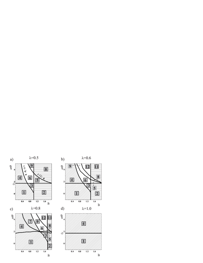
Figure 2: Types of solutions in phase space $\alpha\Theta-\bar{B}$. For $\lambda=1/2$ (a) and $\lambda=1$ (d), the number in each region is given by $N=1+n_{p}+3n_{s}$, where $n_{p}$ is the number of pitchfork bifurcations and $n_{s}$ is the number of bistability regions given by a pair of saddle node bifurcations. The analytic expressions for the limits between regions are shown in some cases. For elliptical polarization (b) and (c), we show a numerical exploration of possible solutions, and we use the number $N=1+n_{p}^{\prime}+3n_{s}$ to identify regions, where $n_{p}^{\prime}$ is the number of saddle node bifurcations that correspond to pitchfork bifurcations for the linear polarization case. The different filling patterns correspond to values of $n_{p}$ or $n_{p}^{\prime}$ equal to 0 (diagonal lines), 1 (horizontal lines) and 2 (white).

Examples of typical solutions are shown in Fig. 3, which also indicates whether the various branches are stable or not under homogeneous perturbations. In order to classify the solutions with a unique index we assign a number, given by $N=1+n_{p}+3n_{s}$, to each possible case.

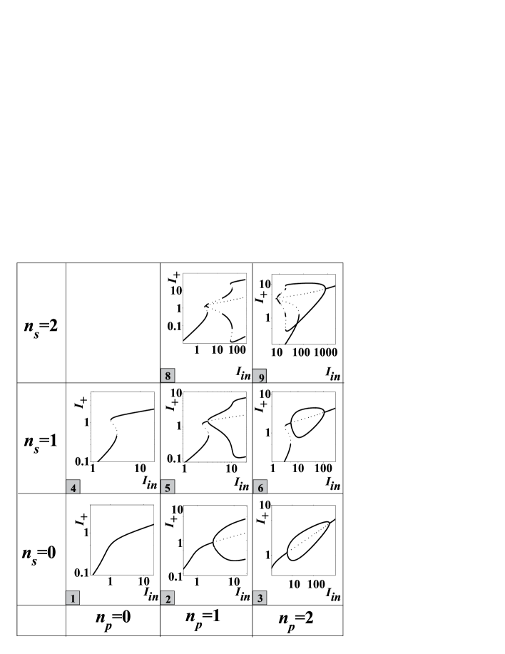
Figure 3: Solutions for $\lambda=1/2$. Full curves were used for showing stable solutions, and dotted curves for unstable solutions. A number $N=1+n_{p}+3n_{s}$ was assigned to each solution (see caption of Fig. 2 for details). Used parameters $(\bar{B},\alpha\Theta)$ are: $N=1$, $(0.4,1)$; $N=2$, $(1.2,1)$; $N=3$, $(0.9,1)$; $N=4$, $(0.4,2.5)$; $N=5$, $(1.2,2.5)$; $N=6$, $(0.6,3)$; $N=8$, $(1.8,2.5)$; $N=9$, $(0.5,7.5)$.

III.2 Circular Polarization, $\lambda=1$

From Eq. (III), it can be shown that if $\lambda=1$, $I_{-}$ is equal to $0$. For $\alpha\Theta<\sqrt{3}$ there is only one possible solution, and, for $\alpha\Theta\geq\sqrt{3}$ there is the well known bistability generated by a couple of saddle-node bifurcations. Possible solution regions are shown in Fig. 2(d). These two only possible solutions for circular polarization are equivalent to solutions 1 and 4 for linear polarization (see Fig. 3).

III.3 Elliptical Polarization, $1/2<\lambda<1$

As we have seen in the previous subsections, there are many possible kinds of solutions for $\lambda=1/2$, but only two for $\lambda=1$. For $1/2<\lambda<1$, up to 11 kinds of solutions were found, but the boundaries of them are related to the roots of degree 9 polynomials, difficulting the derivation of analytical results. However, a numerical search was made for different values of $\lambda$ and some results are shown in Fig. 2(b) (for $\lambda=0.6$), and (c) (for $\lambda=0.8$). An analogy between the types of solution for $\lambda=0.5$ and solution types for $1/2<\lambda<1$ can be drawn, having in mind some considerations. First, there is no longer a symmetric solution: there is only one solution —the connected solution— that exists for $I_{in}\rightarrow 0$ and is continuous for all values of $I_{in}$. Furthermore, instead of appearing or disappearing a couple of asymmetric solutions (as happened for $\lambda=1/2$ through a pitchfork bifurcation), now a couple of unconnected solutions appear or disappear through saddle-node bifurcations. For $I_{in}\rightarrow 0$, if $\lambda=1/2$, only the symmetric solution exists, if $\lambda>1/2$, only the connected solution exists.

All posible cases can be organized in a simple way similar to what we did for $\lambda=1/2$. We define $n_{p}^{\prime}$ as the number of values of $I_{in}$ where there is a saddle-node bifurcation that makes a couple of unconnected solutions appear or disappear (these bifurcations tend to pitchfork bifurcations in the limit $\lambda\rightarrow 1/2$) and $n_{s}$ as the number of regions where bistability occurs due to a couple saddle-node bifurcations.

The possibilities are: only one connected solution ($n_{p}^{\prime}=0$); the connected solution and a couple of unconnected solutions between two values of incident field, produced by two saddle-node bifurcations ($n_{p}^{\prime}=2$); and the connected solution plus a couple of unconnected solutions starting from an incident field value, produced by a single saddle-node bifurcation ($n_{p}^{\prime}=1$). Independently of the value of $n_{p}^{\prime}$, there may be 0, 1 or 2 regions where bistability emerges due to a couple of saddle-node bifurcations on the connected branch ($n_{s}=0$, $1$ or $2$, respectively), or there could be two pairs of saddle-node bifurcations on the connected branch and one on an unconnected branch ($n_{s}=3$). In order to enumerate the cases with a single index, we define $N=1+n_{p}^{\prime}+3n_{s}$. No cases have been found with $n_{s}=3$ and $n_{p}^{\prime}=0$.

There is one case in which there is some ambiguity in the above classification: $n_{p}^{\prime}=1$ (unconnected branches) and $n_{s}=2$ (two regions of bistability). This case corresponds to two qualitatively different solutions: one in which the two bistability regions are on the connected solution (this is the case shown in Fig. 4, solution 8) and the other in which one bistability region is on the connected solution and the other solution is on an unconnected branch. We did not find an equivalent case with $n_{p}^{\prime}=2$ and $n_{s}=2$ where one of the bistability regions is on the lower branch of solutions.

Examples of typical solutions are presented in Figure 4.

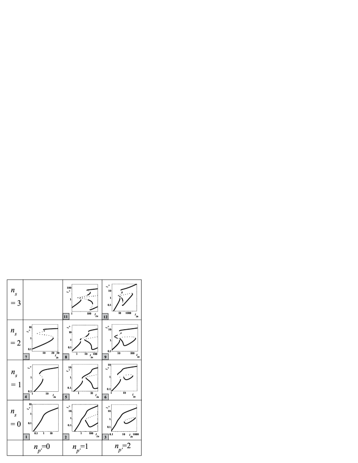
Figure 4: Examples of different solutions for $1/2<\lambda<1$. Full (dotted) line was used for showing stable (unstable) solutions. The number $N=1+n_{p}^{\prime}+3n_{s}$ was assigned to each solution, where $n_{s}$ is the amount of couples of saddle-node bifurcations, and $n_{p}^{\prime}$ is the amount of saddle-node bifurcations where an unconnected couple of solutions start or end. Used parameters $(\bar{B},\alpha\Theta,\lambda)$ were: $N=1$, $(0.4,1,0.7)$; $N=2$, $(1.8,1,0.7)$; $N=3$, $(1.5,1,0.7)$; $N=4$, $(0.4,3,0.7)$; $N=5$, $(1.4,2,0.55)$; $N=6$, $(0.8,3,0.6)$; $N=7$, $(0.6,5,0.7)$; $N=8$, $(1.7,2.2,0.7)$; $N=9$, $(1,4,0.7)$; $N=11$, $(1.8,4,0.7)$; $N=12$, $(1.4,4,0.7)$.

There is a last relevant point about solutions with $\lambda>1/2$: if $n_{p}^{\prime}\geq 1$ a stable unconnected solution with $I_{+}<I_{-}$ may occur. This is a counterintuitive result, since the pumping in the ‘$+$’ polarization is greater than the one in the ‘$-$’ polarization. An example of this phenomenon is analyzed in the next section.

IV Numerical Integration Results

In this section, the temporal evolution of homogeneous solutions of Eq. (12) is studied. In order to do that, numerical simulations applying 4th order Runge-Kutta method are used.

We found that unstable regions in $I_{+}(I_{in})$ graphs are due to three possible reasons. Whenever there is a pair of saddle-node bifurcations, the middle branch will be unstable, and the other two are expected to be stable, as can be seen in, for example, Fig. 3 for $N=4$, or Fig. 4 for $N=4$. If there is a pitchfork bifurcation (or saddle node that generates unconnected solutions), the symmetric branch (or the unconnected middle branch, i.e., the branch closest to the connected solution) will be unstable, and it is expected that the other two solutions are stable, as can be seen in, for example, Fig. 3 for $N=2$ and $3$ or Fig. 4 for the same values of $N$. Finally, there may be areas where we expect a particular branch to be stable, but the solution becomes unstable due to a Hopf bifurcation. Examples of regions where Hopf bifurcations occur can be seen in Fig. 3 for $N=8$ and 9, and Fig. 4 for $N=8$, 9, 11 and 12.

Numerical results show that, if for a given value of $I_{in}$ there is only one unstable solution, due to a couple of saddle-node bifurcations or a pitchfork bifurcation (or saddle-node that generates unconnected solutions), small perturbations in the solution make it evolve to one of the two stable solutions, and the chosen solution depends only on the disturbance. Also, when there is only one solution and it is unstable due to a Hopf bifurcation, a disturbance takes the system to the oscillatory solution. The latter case occurs, for example, with the solution presented in Fig. 4 for $N=8$ and $I_{in}$ between 3 and 7.2. Fig. 5 shows the same case, indicating with arrows the possible values of $I_{+}$ and $I_{-}$ that the unstable solution takes after it is perturbed. It is important to note that the Hopf oscillation occurs in a four-dimensional space generated by the real and imaginary parts of $A_{+}$ and $A_{-}$, and the present graph shows only the square modules of those fields.

Interesting behaviors occur when, for a given $I_{in}$ value, there are two or more unstable solutions, due to bifurcations generated by instabilities of the same or different types. For instance, it can be seen in Fig. 5, for $I_{in}=20$, that the unstable unconnected solution evolves towards the stable unconnected solution or to the closest stable connected solution (but it does not evolve to the other stable connected solution). Also, in the same figure and for the same value of $I_{in}$, the unstable connected solution (the dotted part of the connected solution, which occurs due to a couple of saddle node bifurcations on the connected solution) evolves towards one of the two stable connected solutions (it does not go towards the unconnected stable solution).

Figure 5: Example of evolution of unstable solutions (parameters as in Fig. 4, $N=8$). It can be seen that, for the stable unconnected solution, $I_{-}>I_{+}$ although the input field has $|A_{in+}|^{2}>|A_{in-}|^{2}$. Full (dotted) line is for stable (unstable) stationary solutions, and gray regions are for oscillations due to a Hopf bifurcation. Arrows show the evolution of a perturbed unstable solution for some typical cases. For $I_{in}=2.5$, the unstable solution related to a couple of saddle-node bifurcations —UC1— evolves into one of the two stable solutions —SC1 or SC2—. For $I_{in}=9$, if the system starts at the connected unstable solution —H—, it evolves towards the Hopf oscillation; if the system starts at the unconnected unstable solution —UU1— , it can evolve to the lower stable solution —SU1— or to the Hopf bifurcation —H—. For $I_{in}=20$, perturbations around the unstable point of the connected solution —UC2— make the system evolve to the stable points of the same connected solution —SC3 or SC4—; the unconnected unstable branch —UU2— evolves towards the stable unconnected branch —SU2— or towards the closest stable point of the connected solution —SC3, it does not evolve towards SC4—.

V Conclusions

We described the evolution of the electromagnetic field in a ring cavity with flat mirrors, filled with a Kerr-type electric and magnetic nonlinear material with positive or negative refraction index. We took into account the degree of freedom of the polarization of the incident field. Starting from two pairs of coupled nonlinear Schrödinger equations (for the circularly left and right polarized components of the electric and magnetic fields), we found a proportionality relation between electric and magnetic field components, so that the description was reduced to just two Lugiato Lefever equations.

Considering that the effective magnetic response can be nonlinear, and taking into account the polarization degree of freedom of the incident beam, a rich variety of possible bifurcations in homogeneous stationary solutions was found, depending on the values of the constants that describe the system. These solutions were classified and exemplified. The number of qualitatively different solutions that were obtained is large, and our classification in terms of the number of possible bifurcations simplifies the description.

In the case of linear polarization ($\lambda=1/2$), we found that the solutions $I_{+}$ and $I_{-}$ depending on $I_{in}$, could present between 0 and 2 pitchfork bifurcations and between 0 and 2 pairs of saddle-node bifurcations, yielding 8 possible cases. We determined the boundaries between regions of each type of solution in the parameter space given by $\alpha\Theta$ and $\bar{B}$. The same analysis was performed for circular polarization ($\lambda=1$).

For elliptical polarization ($1/2<\lambda<1$), we found 11 possible cases based on the number of bifurcations. We numerically explored regions of parameters that generated each case.

We also numerically analyzed how unstable homogeneous solutions evolve after a disturbance, and found regions where Hopf instabilities take place.

Finally, for elliptical polarization there are some sets of parameters where, taking an incident field polarized mostly in the ‘$+$’ component, it is possible to obtain stable solutions where the ‘$-$’ polarization component prevails.

In summary, we presented an analysis of the possible homogeneous stationary solutions of the electromagnetic field in a ring cavity containing a material with electric and magnetic nonlinearities, and taking into account the polarization degree of freedom of the light. Let us note that even for linearly polarized incident light, elliptically polarized solutions can appear, so that considering only a scalar equation may cause the removal of a possible solution. Despite the large number of parameters of the original description, a classification of the possible solutions for a given polarization could be obtained taking into account only two parameters: $\alpha$ (related to the sign of the electric and magnetic nonlinear susceptibilities) times $\Theta$ (the scaled detuning) and $\bar{B}$ (related to the electric and magnetic nonlinear constants $B_{E}$ and $B_{M}$). Results presented here can be useful when ring cavities are used in optical switching or information storage.

- (1) D.R. Smith, W.J. Padilla, D.C. Vier, S.C. Nemat-Nasser and S. Schultz, Phys. Rev. Lett. 84 4184 (2000)
- (2) R.A. Shelby, D.R. Smith and S. Schultz, Science 292 77 (2001).
- (3) J.V. Moloney and A.C. Newell, Nonlinear Optics (Westview Press, Boulder, Colorado, 2003).
- (4) Z.-H. Xiao, K.Kim, Optics Comunications 283 (2010) 2178-2181.
- (5) M. A. Antón, O. G. Calderón, S. Melle, I. Gonzalo, F. Carreño Optics Comunications 268 (2006) 146-154.
- (6) P. Kockaert, P. Tassin, G. Van der Sande, I. Veretennicoff and M. Tlidi, Phys. Rev. A 74, 033822 (2006); P. Tassin, L. Gelens, J. Danckaert, I. Veretennicoff, P. Kockaert and M. Tlidi, Chaos 17, 037116 (2007).
- (7) P. Tassin, G. Van der Sande, I. Veretennicoff, M. Tlidi and P. Kockaert, Proc. SPIE 5955, 59550X (2005).
- (8) S. Wen, Y. Wang, W. Su, Y. Xiang. X. Fu and D. Fan, Phys. Rev. E 73, 036617 (2006).
- (9) M. Scalora, M.S. Syrchin, N. Akozbek, E.Y. Poliakov, G. D’Aguanno, N. Mattiucci, M.J. Bloemer and A.M. Zheltikov, Phys. Rev. Lett. 95, 013902 (2005).
- (10) N. Lazarides and G.P. Tsironis, Phys. Rev. E 71, 036614 (2005); I. Kourakis and P.K. Shukla, Phys. Rev. E 72, 016626 (2005).
- (11) R. Merlin, PNAS 2009 106 (6) 1693-1698.
- (12) M. Lapine, M. Gorkunov, and K. H. Ringhofer, Phys. Rev. E 67, 065601 (2003).
- (13) A.A. Zharov, I.V. Shadrivov and Y.S. Kivshar, Phys. Rev. Lett 91, 037401 (2003).
- (14) D. A. Martin, M Hoyuelos Phys. Rev. E 80, 056601 (2009)
- (15) L.A. Lugiato and R. Lefever, Phys. Rev. Lett. 58, 2209 (1987); L.A. Lugiato, W. Kaige and N.B. Abraham, Phys. Rev. A 49, 2049 (1994).
- (16) W.J. Firth, A.J. Scroggie, G.S. McDonald and L. Lugiato, Phys. Rev. A 46, R3609 (1992); J.B. Geddes, J.V. Moloney, E.M. Wright and W.J. Firth, Opt. Commun. 111, 623 (1994).
- (17) M. Hoyuelos, P. Colet, M. San Miguel and D. Walgraef, Phys. Rev. E 58, 2992 (1998).
- (18) C. L. Holloway, E. F. Kuester, J. Baker-Jarvis and Pavel Kabos, IEEE Transactions on antennas and propagation 51, 10 (2003)
- (19) X. Cai, R. Zhu and G. Hu, Metamaterials 2, 220 (2008).
- (20) Th. Koschny, L. Zhang and C. M. Soukoulis, Phys. Rev. B 71, 121103(R) (2005) .
- (21) J. B. Geddes, J. V. Moloney, E. M. Wright, and W. J. Firth, Opt. Commun. 111, 623 (1994).
- (22) V.G. Veselago, Usp. Fiz. Nauk 92 517 (1967); V.G. Veselago, Sov. Phys.-Usp. 10 509 (1968).
- (23) R. W. Boyd, Nonlinear Optics 2nd Ed. (Academic Press, San Diego, California, 2003).
- (24) R. Liu, A. Degiron, J. J. Mock and D. R. Smith, Appl. Phys. Lett. 90, 263504 (2007).
- (25) Wang Jia-Fu, Qu Shao-Bo, Xu Zhuo, Zhang Jie-Qiu, Ma Hua, Yang Yi-Ming and Gu Chao, Chinese Phys. Lett. 26, 084103 (2009).
- (26) G. Dolling, M. Wegener, C. M. Soukoulis, and S. Linden, Opt. Express 15, 11536-11541 (2007).
- (27) V. M. Shalaev, T. A. Klar, V. P. Drachev, and A. V. Kildishev, Optical Negative-Index Metamaterials: From Low to No Loss, in Photonic Metamaterials: From Random to Periodic, Technical Digest (CD) (Optical Society of America, 2006), paper TuC3.
- (28) A. K. Popov and V. M. Shalaev, Optics Letters 31, 2169-2171 (2006).